Maximized Privacy-Preserving Outsourcing on Support Vector Clustering

Abstract

Despite its remarkable capability in handling arbitrary cluster shapes, support vector clustering (SVC) suffers from pricey storage of kernel matrix and costly computations. Outsourcing data or function on demand is intuitively expected, yet it raises a great violation of privacy. We propose maximized privacy-preserving outsourcing on SVC (MPPSVC), which, to the best of our knowledge, is the first all-phase outsourceable solution. For privacy-preserving, we exploit the properties of homomorphic encryption and secure two-party computation. To break through the operation limitation, we propose a reformative SVC with elementary operations (RSVC-EO, the core of MPPSVC), in which a series of designs make selective outsourcing phase possible. In the training phase, we develop a dual coordinate descent solver, which avoids interactions before getting the encrypted coefficient vector. In the labeling phase, we design a fresh convex decomposition cluster labeling, by which no iteration is required by convex decomposition and no sampling checks exist in connectivity analysis. Afterward, we customize secure protocols to match these operations for essential interactions in the encrypted domain. Considering the privacy-preserving property and efficiency in a semi-honest environment, we proved MPPSVC’s robustness against adversarial attacks. Our experimental results confirm that MPPSVC achieves comparable accuracies to RSVC-EO, which outperforms the state-of-the-art variants of SVC.

1. Introduction

Clustering forms natural groupings of data samples that maximize intra-cluster similarity and minimize inter-cluster similarity. Inspired by support vector machines (SVMs), support vector clustering (SVC) has attracted many studies for remarkably handling clusters with arbitrary shape [1,2,3,4]. Various application areas are closely related to it, e.g., information retrieval and analysis, signal processing, traffic behavior identification, etc. [2,4,5,6]. However, building a good clustering model requires a large number of valid training samples and a substantial iterative analysis under specific metrics; hence, it is frequently hard for individuals or small organizations to build their model on those quickly accumulated data. The pricey storage of the kernel matrix and costly computations by the dual problem solver and a large number of sampling checks set big barriers to its applications [4,7,8]. To tackle this issue, a viable solution is to outsource its heavy workloads to the Cloud [9] with sufficient computing resources. With suitable outsourcing techniques, the excess requirements of computational and storage resources for data owners can be mitigated to the Cloud.

By introducing Cloud computing, a server (in logical) in the Cloud takes the place of the client (data owner) to finish either the training phase or the labeling phase, or both. After all, as a third-party, the credibility of servers cannot be fully guaranteed. The undertaken tasks are remotely based on privately owned data samples. Furthermore, there is no need for the server to disclose any details or negotiate parameters of the analysis, even if it offers a clustering service to the client. Hence, using a third-party to build or utilize models on sensitive data is risky even if the service provider claims that it will not observe the analysis [10,11]. It is crucial to develop a privacy-preserving SVC which seeks a server to train the model and label data samples while guaranteeing the privacy, i.e., the input data, the coefficient vector, and the labeling results.

In this paper, we propose, to the best of our knowledge, the first known client–server privacy-preserving SVC architecture, namely maximized privacy-preserving outsourcing on SVC (MPPSVC), to maximize the benefits of the emerging Cloud computing technology in cluster analysis. As shown in Figure 1, the client first sends a protected diagonal matrix to the server; then, the server employs a reformative SVC framework to perform the dual problem solver in the encrypted-domain (ED) and sends the encrypted coefficient vector back. To let the client know the cluster prototype and the labeling results, we first cut off the traditional iterative analysis for efficiency and securely exploit the homomorphic encryption properties. Then, we design lightweight secure protocols which require a limited number of interactions. We assume that both the client and the server execute the protocol correctly to maintain their reputation; hence, they will behave in a semi-honest manner, i.e., they are honest but curious, thus privacy is a real issue. The main contributions of this work lie in:

(1)

A reformative SVC with elementary operations (RSVC-EO) is proposed with an updated dual coordinate descent (DCD) solver for the dual problem. In the training phase, it prefers a linear method to approach the objective without losing validity. Furthermore, it easily trades time for space by calculating kernel values on demand.

(2)

A fresh convex decomposition clustering labeling (FCDCL) method is presented, by which iterations are not required for convex decomposition. In connectivity analysis, the traditional segmer sampling checks in feature space are also avoided. Consequently, to complete calculations in each step of the outsourcing scene, a single interaction is sufficient for prototype finding and connectivity analysis. Without a mass of essential iterations, the labeling phase will not hurt the outsourcing.

(3)

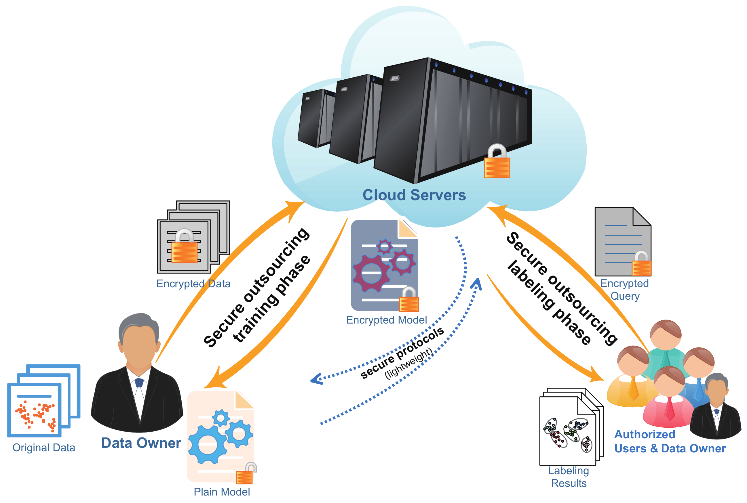
Towards privacy-preserving, MPPSVC is proposed by introducing homomorphic encryption, two-party computation, and linear transformation to reconstruct RSVC-EO. Although these protocols limit the calculation types, MPPSVC works well with maximized outsourcing capability. In the field of SVC, to the best of our knowledge, it is the first known client–server privacy-preserving clustering framework solving the dual problem without interaction. Furthermore, it can securely outsource the cluster number analysis and cluster assignment on demand.

The remainder of the paper is organized as follows. Section 2 briefly describes the classic SVC and the homomorphic encryption and discusses the privacy violation and limited operations of SVC outsourcing. In Section 3, we first reformulate the dual problem and propose the DCD solver to it. Meanwhile, we present FCDCL that completes convex decomposition without iterative analysis and finishes connectivity analysis irrespective of sampling. By integrating these designs, we give an implementation of RSVC-EO in plain-domain (PD). Section 4 proposes MPPSVC for the client–server environment in ED, and presents the core idea of securely outsourcing the three crucial tasks of RSVC-EO. Section 5 gives performance and security analysis for these ED techniques. Section 6 reviews the related works. Finally, the conclusions are drawn in the Section 7, as well as the future works to be investigated.

2. Preliminaries

2.1. Support Vector Clustering

2.1.1. Estimation of a Trained Support Function

Assume that a dataset $\mathcal{X}$ has N data samples $\{{\mathbf{x}}_1,\dots ,{\mathbf{x}}_N\}$, where ${\mathbf{x}}_i\in {\mathbb{R}}^d$ with $i\in [1,N]$. Through a nonlinear function $\mathsf{\Phi }(·)$, SVC maps data samples from data space to a high-dimensional feature space and finds a sphere with the minimal radius which contains most of the mapped data samples. This sphere, when mapped back to the data space, can be partitioned into several components, each enclosing an isolated cluster of samples. In mathematical formulation, the spherical radius R is subject to

$$\begin{array}{cc}\hfill & \underset{R,\alpha ,{\xi }_i}{min}{R}^2+C\sum _i{\xi }_i\hfill \\ \hfill & \mathrm{s}.\mathrm{t}.\left|\right|\mathsf{\Phi }\left({\mathbf{x}}_i\right)-\mathbf{\alpha }{\left|\right|}^2\le R^2+{\xi }_i\hfill \end{array}$$

(1)

where $\mathbf{\alpha }$ is the sphere center, ${\xi }_i$ is a slack variable, and C is a constant controlling the penalty of noise. Following Jung et al. [12], the sphere can be simply estimated by a support function that is defined as a positive scalar function $f:{\mathbb{R}}^n\to {\mathbb{R}}^{+}$. After solving the dual problem in Equation (2), we estimate the support function by support vectors (SVs) whose corresponding coefficients ${\beta }_i\in (0,C)$ for $i=1,\dots ,N$.

$$\begin{array}{cc}\hfill & \underset{{\beta }_j}{min}\sum _{i,j}{\beta }_i{\beta }_{j}K({\mathbf{x}}_i,{\mathbf{x}}_j)-\sum _{j}K({\mathbf{x}}_j,{\mathbf{x}}_j){\beta }_j\hfill \\ \hfill & \mathrm{s}.\mathrm{t}.\sum _j{\beta }_j=1,0\le {\beta }_j\le C,j=1,\dots ,N\hfill \end{array}$$

(2)

By optimizing Equation (2) with Gaussian kernel $K({\mathbf{x}}_i,{\mathbf{x}}_j)=e^{-q\left|\right|{\mathbf{x}}_i-{\mathbf{x}}_j{\left|\right|}^2}$, the objective trained support function is formulated by

$$f\left(\mathbf{x}\right)=1-2\sum _j{\beta }_{j}K({\mathbf{x}}_j,\mathbf{x})+\sum _{i,j}{\beta }_i{\beta }_{j}K({\mathbf{x}}_i,{\mathbf{x}}_j).$$

(3)

Theoretically, the radius R of the hypersphere is usually defined by the square root of $f\left({\mathbf{x}}_i\right)$ where ${\mathbf{x}}_i$ is one of SVs.

2.1.2. Cluster Assignments

Since SVs locate on the border of clusters, a simple graphical connected-component method can be used for cluster labeling. For any two samples, ${\mathbf{x}}_i$ and ${\mathbf{x}}_j$, we check m segmers on the line segment connecting them by traveling their images in the hypersphere. According to Equation (3), ${\mathbf{x}}_i$ and ${\mathbf{x}}_j$ should be labeled the same cluster index if all the m segmers are always lying in the hypersphere, i.e., $f\left({\mathbf{x}}_{\tilde{m}}\right)\le R^2$ for $\tilde{m}\in [1,m]$. Otherwise, they are in two different clusters.

2.2. Homomorphic Encryption

Multiplication is critical for SVC. Although the fully homomorphic encryption protects multiplicative items well, the existing schemes are far from practical use. Since multiplication can be replaced by addition, we prefer using the Paillier cryptosystem [13]—an additively homomorphic public-key encryption scheme—to secure clustering analysis and data exchange. It was also adopted by the authors of [14,15,16,17,18] for simplicity and generality. Based on the decisional composite residuosity problem, the Paillier cryptosystem is provable semantic security. It means that, for some composite n, we cannot decide whether there exists some $y\in {\mathbb{Z}}_{n^2}^{*}$ such that an integer z satisfies $z=y^{n}mod{n}^2$. A brief description of the Paillier cryptosystem is given as follows.

Let $n=pq$ where p and q are two large primes, r is randomly selected in ${\mathcal{Z}}_n^{*}$, and g is randomly selected in ${\mathcal{Z}}_{n^2}^{*}$, which satisfies $gcd(L(g^{\lambda }mod{n}^2),n)=1$ with $L\left(u\right)=\frac{u-1}{n}$ and $\lambda =\mathrm{lcm}(p-1,q-1)$. We assume that plaintext $m\in {\mathcal{Z}}_n$ is the numeric form of a feature value in ${\mathbf{x}}_i(i=1,\cdots ,N)$; its ciphertext is denoted by $\left[\right[m\left]\right]$, i.e., $\left[\left[m\right]\right]\in {\mathcal{Z}}_{n^2}^{*}$. The Paillier cryptosystem’s encryption, decryption, and additively homomorphic operations are as follows:

(1)

Encryption: Ciphertext $\left[\left[m\right]\right]=g^m·r^{n}mod{n}^2$.

(2)

Decryption: Plaintext $m=(L(\left[\left[m\right]\right]mod{n}^2)/L(g^{\lambda }mod{n}^2))modn$.

(3)

Additive homomorphism: $\left[[m_1+m_2]\right]=\left[\left[m_1\right]\right]·\left[\left[m_2\right]\right]$, $\left[[\alpha ·m_1]\right]={\left[\left[m_1\right]\right]}^{\alpha }$. Here, $m_1$ and $m_2$ are two numeric features in PD and $\alpha$ is an integer constant. In practical situations, if $\alpha <0$, its equivalence class value $\alpha modn$ can be a substitution.

Before outsourcing data, in this study, the client should distribute his public key (i.e., $(n,g)$) of the predefined Paillier cryptosystem to the server while keeping his private key (i.e., $(p,q,r)$ or $(\lambda ,r)$) secret. Then, the server performs a series of clustering tasks on ciphertexts by exploiting the homomorphic properties. Only the client can decrypt all the encrypted messages that encapsulate clustering results by using his corresponding private key.

2.3. Privacy Violation and Limited Operations of SVC Outsourcing

2.3.1. Privacy Violation of SVC

Undoubtedly, to conduct the essential computations of SVC correctly in the Cloud, we have to face the possibility of privacy leakage in either the training phase or the labeling phase, or both. Otherwise, there is no feasibility.

For the training phase, the core work is to solve the dual problem in Equation (2). After being transferred to the Cloud, in PD, either the data samples or the kernel matrix is undoubtedly retrievable for the server. Based on privacy-preserving policy, this situation raises several critical problems. (1) Letting the server know the data samples as plaintext is unacceptable. (2) Only having separately encrypted data samples, the server cannot generate the required kernel matrix by itself, since calculating the Gaussian function needs the help from the client, as discussed by Rahulamathavan et al. [17]. However, more than $N^2$ times interactions between the server and the client are required before the server constructs a $N\times N$ kernel matrix. Besides, the widely used SMO solver for solving the dual problem needs approximately $O\left(N^2\right)$ kernel evaluations to construct the support function [8]. Taking the number of iterations ℓ into account, far more than $N^2$ times interactions are also essential for the SMO solver. Therefore, it is inadvisable to encrypt data samples separately. (3) To make the solver iterate effectively, the intermediate results of the coefficient vector should be in PD. Unfortunately, this would leak the final index of SVs with their importance to the server. (4) Although no plain data samples appear, the constructed kernel matrix is not suitable to be sent to the server directly. If the server knows any data sample, it can recover all the data samples since the kernel function is exactly a type of similarity measure [19].

For the labeling phase, labeling the remaining data samples, usually based on the Euclidean distances in data space, is not a time-consuming work if the cluster prototypes have been obtained. Samanthula et al. [20] presented a good idea for it, even though we have to do it in an outsourced environment. However, in the most recent studies, prototype finding and sampling calculation for connectivity analysis generally are based on iterative analysis, which raises frequent interactions to get help from the client because exponent arithmetic is the fundamental operation, and SVs are the component of the exponent function (i.e., support function). Otherwise, privacy cannot be guaranteed. It is worth mentioning that Lin and Chen [21] presented a method of releasing the training SVM classifier without violating the confidentiality of classification parameters, e.g., SVs. Although replacing the trained SVM classifier by the support function appears to be a good solution, unfortunately, we still have to send the plain data samples for decisions made by the outsourced service in the server. Undoubtedly, this results in a privacy violation.

2.3.2. Limited Operations of Homomorphic Encryption

As described in Section 2.2, additively homomorphic encryption is characterized by its additive homomorphism. However, this fundamental operation only expedites the addition operation for two ciphertexts and the multiplication operation between a plaintext and a ciphertext. Therefore, without outside assistance, it still cannot complete multiplication/division operations for two plaintext or complex functions, e.g., Gaussian function. Unfortunately, multiplication/division operations are frequently invoked by both the SMO solver and iterative analysis for cluster prototypes. Furthermore, calculating values of Gaussian function with different sample pairs is a fundamental operation in the SMO solver, iterative analysis for cluster prototypes, and sampling for connectivity analysis. Since the client is the only legal assistance provider outside, this will dramatically raise the huge scope of interactions that lead to heavy load to network bandwidth and degrade the usability of SVC outsourcing. Therefore, it is critical to explore practical ways of avoiding too many complex computations and massive interactions.

3. Reformative Support Vector Clustering with Elementary Operations

Traditionally, iterative analysis and complex operations cause massive interactions that reduce the usability of outsourcing. Towards balancing privacy, efficiency, and accuracy, we design the DCD solver by reducing unnecessary operations and replacing complex functions by elementary ones, and we also design the FCDCL to avoid iterative analysis in convex decomposition and connectivity analysis.

3.1. DCD Solver for SVC’s Dual Problem

Derived from [22], we reformulate the nonlinear dual problem in Equation (2) by a linear model. Let Q be the original kernel matrix with element $Q_{ij}=K({\mathbf{x}}_i,{\mathbf{x}}_j)(i,j\in [1,N])$, $\tilde{Q}=2\times Q$, $\mathit{\beta }={[{\beta }_1,{\beta }_2,\cdots ,{\beta }_N]}^T$, and $\mathbf{e}={[1,1,\cdots ,1]}^T$. Since $K({\mathbf{x}}_i,{\mathbf{x}}_j)=1$ for ${\mathbf{x}}_i={\mathbf{x}}_j$, we have ${\sum }_{j}K({\mathbf{x}}_j,{\mathbf{x}}_j){\beta }_j=1$. Then, the dual problem in Equation (2) can be reformulated by

$$\begin{array}{cc}\hfill & \underset{\mathit{\beta }}{min}\frac{1}{2}{\mathit{\beta }}^T\tilde{Q}\mathit{\beta }-1\hfill \\ \hfill & \mathrm{s}.\mathrm{t}.\sum _j{\beta }_j=1,0\le {\beta }_j\le C,j=1,\dots ,N.\hfill \end{array}$$

(4)

Let $D_{\mathrm{svc}}$ denote $\left\{\mathit{\beta }\right|{\sum }_j{\beta }_j=1,0\le {\beta }_j\le C,j=1,\dots ,N\}$. Obviously, we can relax $D_{\mathrm{svc}}$ by $D_{\mathrm{svc}}^{\prime }=\left\{\mathit{\beta }\right|0\le {\beta }_j\le C,j=1,\dots ,N\}$ in which an equivalent globally optimal solution can be achieved. We thus get an equivalent form of the problem in Equation (2) as

$$\begin{array}{cc}\hfill & \underset{\mathit{\beta }}{min}\frac{1}{2}{\mathit{\beta }}^T\tilde{Q}\mathit{\beta }\hfill \\ \hfill & \mathrm{s}.\mathrm{t}.0\le {\beta }_j\le C,j=1,\dots ,N.\hfill \end{array}$$

(5)

Without any prior knowledge of labels, we fix the label $y_i$ of ${\mathbf{x}}_i$ to $+1$ or $-1$ for $i=1,\cdots ,N$. To solve the problem in Equation (5), the optimization process starts from an initial point ${\mathit{\beta }}^0\in R^N$ and generates a sequence of vectors ${\left\{{\mathit{\beta }}^k\right\}}_{k=1}^{\infty }$. We refer to the process from ${\mathit{\beta }}^k$ to ${\mathit{\beta }}^{k+1}$ as an outer iteration. In each outer iteration, we have N inner iterations, so that sequentially ${\beta }_1,{\beta }_2,\cdots ,{\beta }_N$ are updated. Each outer iteration thus generates vectors ${\mathit{\beta }}^{k,i}\in R^N,i=1,2,\cdots ,N+1$, such that ${\mathit{\beta }}^{k,1}={\mathit{\beta }}^k$, ${\mathit{\beta }}^{k,N+1}={\mathit{\beta }}^{k+1}$, and ${\mathit{\beta }}^{k,i}={[{\beta }_1^{k+1},\dots ,{\beta }_{i-1}^{k+1},{\beta }_i^k,\dots ,{\beta }_N^k]}^T$ for $\forall i=2,\dots ,N$. To update ${\mathit{\beta }}^{k,i}$ to ${\mathit{\beta }}^{k,i+1}$, we fix the other variable and then solve the following one-variable sub-problem:

$$\begin{array}{cc}\hfill & \underset{d}{min}f({\mathit{\beta }}^{k,i}+\theta {\mathit{e}}_i)\hfill \\ \hfill & \mathrm{s}.\mathrm{t}.0\le {\beta }_i^k+d\le C,\hfill \end{array}$$

(6)

where ${\mathit{e}}_i={[0,\dots ,0,1,0,\dots ,0]}^T$. Then, the objective function of Equation (6) is a simple quadratic function of $\theta$:

$$f({\mathit{\beta }}^{k,i}+\theta {\mathit{e}}_i)=\frac{1}{2}{\tilde{Q}}_{ii}{d}^2+{\mathsf{\nabla }}_{i}f\left({\mathit{\beta }}^{k,i}\right)\theta +\mathrm{constant},$$

(7)

where ${\mathsf{\nabla }}_{i}f$ is the ith component of the gradient $\mathsf{\nabla }f$. Therefore, based on a decision function definition of $y={\mathit{w}}^T\mathsf{\Phi }\left(\mathbf{x}\right)+b$ for SVC, we can solve problem in Equation (7) by introducing Equations (8)–(9).

$${\tilde{Q}}_{ii}=2\times K({\mathbf{x}}_i,{\mathbf{x}}_i)=2.$$

(8)

$${\mathsf{\nabla }}_{i}f\left(\mathit{\beta }\right)={\left(\tilde{Q}\mathit{\beta }\right)}_i=\sum _{j=1}^N{\tilde{Q}}_{ij}{\beta }_j={\mathit{w}}^T\mathsf{\Phi }\left({\mathbf{x}}_i\right).$$

(9)

Along with the update of ${\beta }_i$, we can maintain $\mathit{w}$ by

$$\mathit{w}\leftarrow \mathit{w}+({\beta }_i-{\widehat{\beta }}_i)\mathsf{\Phi }\left({\mathbf{x}}_i\right),$$

(10)

where ${\widehat{\beta }}_i$ is the temporary coefficient value obtained in the previous iteration. Thus, we have

$${\mathsf{\nabla }}_{i}f\left({\mathit{\beta }}^{k,i}\right)\leftarrow \underset{(k-1)\mathrm{iter}.}{\underbrace{{\sum }_j\widehat{{\beta }_j}K({\mathbf{x}}_j,{\mathbf{x}}_i)}}+(\beta -{\widehat{\beta }}_i).$$

(11)

Therefore, similar to the DCD method in [22], we propose a DCD solver detailed by Algorithm 1 for solving the problem in Equation (2). Briefly, we use Equation (11) to compute ${\mathsf{\nabla }}_{i}f\left({\mathit{\beta }}^{k,i}\right)$, check the optimality of the single-variable optimization in Equation (6) by ${\mathsf{\nabla }}_i^{P}f\left({\mathit{\beta }}^{k,i}\right)\stackrel{?}{>}1\times {10}^{-12}$, and update ${\beta }_i$. The cost per iteration from ${\mathit{\beta }}^k$ to ${\mathit{\beta }}^{k+1}$ is $O\left(Nd\right)$, and an appropriate $ϵ$ controls the iteration number well for efficiency. Notice that the memory requirement is flexible. With sufficient memory, we can afford $O\left(N^2\right)$ for the full kernel matrix, and use search on demand to finish the calculation of line 5 in Algorithm 1; otherwise we can either store $\mathcal{X}$ or split them into blocks (requirement reduced to $\le O\left(N\right)$), and then calculate the values of required kernel function sequentially for later use in the outer iterations.

Algorithm 1 DCD solver for SVC’s dual problem in Equation (2).

Require: Dataset $\mathcal{X}$, kernel width q, and penalty C Ensure: Coefficient vector $\mathit{\beta }$ 1. Randomly initialize the coefficient vector $\mathit{\beta }$ 2. while true do 3.  $M_{\mathrm{ax}}\leftarrow -\infty$, $M_{\mathrm{in}}\leftarrow \infty$ 4.  for$i=1,2,\dots ,N$do 5.   $\widehat{G}=2\times {\sum }_{j=1}^N{\beta }_{j}K({\mathbf{x}}_j,{\mathbf{x}}_i)$ 6.   $G\leftarrow \widehat{G}+({\beta }_i-{\widehat{\beta }}_i)$ 7.   $PG=\left\{\begin{array}{cc}G\hfill & \mathrm{if}0<{\beta }_i<C\hfill \\ min(G,0)\hfill & \mathrm{if}{\beta }_i=0\hfill \\ max(G,0)\hfill & \mathrm{if}{\beta }_i=C\hfill \end{array}\right.$ 8.   $M_{\mathrm{ax}}\leftarrow max(M_{\mathrm{ax}},\left|PG\right|)$, $M_{\mathrm{in}}\leftarrow min(M_{\mathrm{in}},\left|PG\right|)$ 9.   if$\left|PG\right|>$ 1E-12 then 10.    ${\widehat{\beta }}_i\leftarrow {\beta }_i$ 11.    ${\beta }_i\leftarrow min(max({\beta }_i-\frac{1}{2}G,0),C)$ 12.   end if 13.  end for 14.  if$(M_{\mathrm{ax}}-M_{\mathrm{in}})\le ϵ$then 15.   break 16.  end if 17. end while

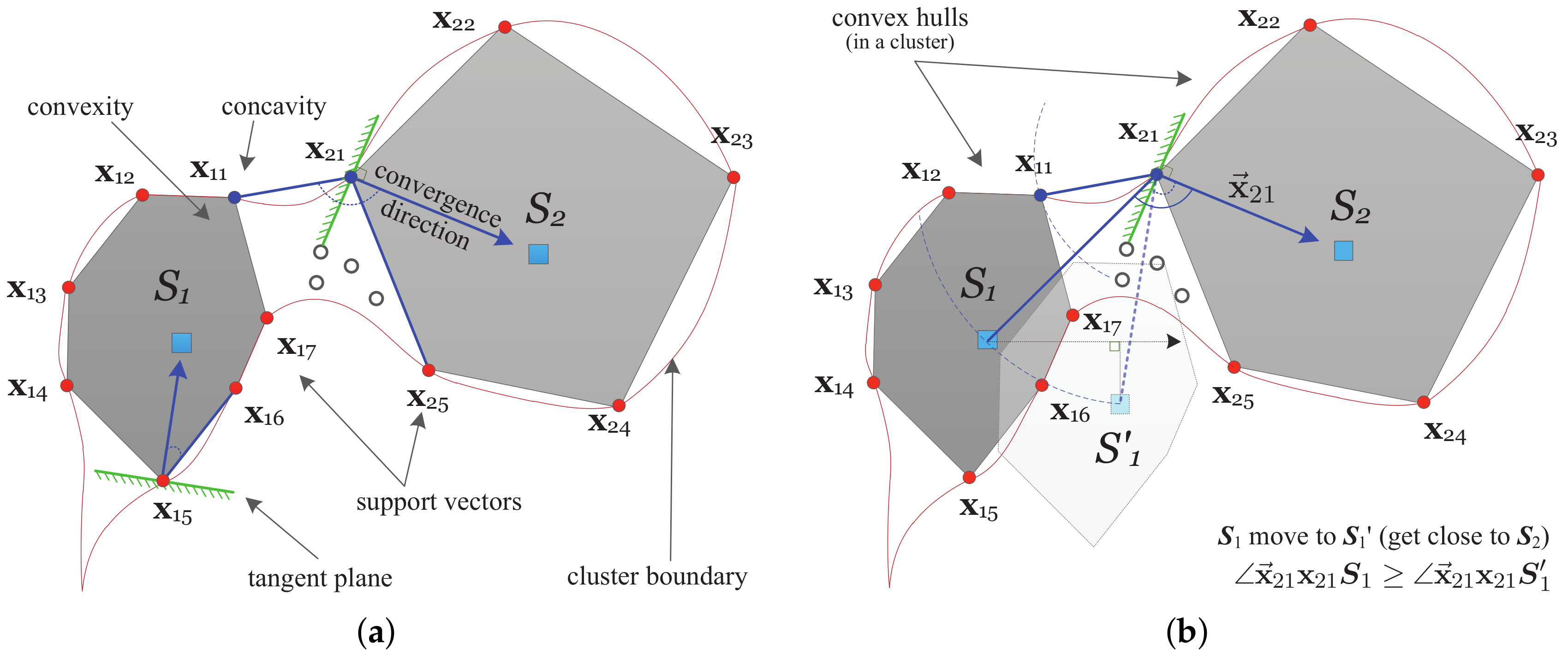
3.2. Convex Decomposition without Iterative Analysis

Derived from [22], in the labeling phase, we take convex hull as the cluster prototype for both efficiency and accuracy. However, it usually requires $\ell (\gg 1)$ iterations to get a stable equilibrium vector (SEV) from an SV. If we let the server do this, the client has to finish the exponential function by itself. Combining with the uncertain number of SVs $N_{\mathrm{SV}}$, more than $\ell N_{\mathrm{SV}}$ rounds of interactions bring a heavy burden to the network bandwidth. Therefore, we prefer achieving the same object without iterative analysis.

Theorem 1.

If a cluster is decomposed into multiple convex hulls, the best division positions should be those SVs whose locations link up two nearest neighboring convexity and concavity.

Proof. 

From the convex decomposition strategy [23], theoretically, the decomposed convex hulls are constructed by SVs without exceptions. Taking Figure 2a as an example, ${\mathit{S}}_1$ and ${\mathit{S}}_2$, respectively, denote the two convex hulls in a cluster and the corresponding SEVs. Obviously, the cluster is stroked SVs $\{{\mathbf{x}}_{11},\cdots ,{\mathbf{x}}_{17};{\mathbf{x}}_{21},\cdots ,{\mathbf{x}}_{25}\}$. $\{{\mathbf{x}}_{11},{\mathbf{x}}_{17}\}$ and $\{{\mathbf{x}}_{21},{\mathbf{x}}_{25}\}$ constitute the division position (termed division set) for linking up two nearest neighboring convexity and concavity. To confirm this, we consider the two situations:

(1)

If the division position is not in the SVs subset in which each one links up two nearest neighboring convexity and concavity, for instance, ${\mathbf{x}}_{21}$ is replaced by ${\mathbf{x}}_{22}$, then the corresponding convex hull ${\mathit{S}}_2$ has to be further split into two convex hulls enclosed by $\{{\mathbf{x}}_{21},{\mathbf{x}}_{22},{\mathbf{x}}_{25}\}$ and $\{{\mathbf{x}}_{22}^{\prime },{\mathbf{x}}_{23},{\mathbf{x}}_{24}\}$, respectively, even though all these SVs converge to ${\mathit{S}}_2$. Here, ${\mathbf{x}}_{22}^{\prime }$ is an imaginary sample that is extremely similar to ${\mathbf{x}}_{22}$. Because no overlapping region or intersection of vertices of convex hulls is allowed, unfortunately, this result conflicts with the definition that SVs in a convex hull will converge to the same SEV.

(2)

From the other perspective, if ${\mathbf{x}}_{21}$ is not in the division position which only includes $\{{\mathbf{x}}_{11},{\mathbf{x}}_{17},{\mathbf{x}}_{25}\}$, we have to find a substitute ${\mathbf{x}}_{21}^{\prime }$ to construct the convex hull ${\mathit{S}}_2$. ${\mathbf{x}}_{21}^{\prime }$ might locate between ${\mathbf{x}}_{11}$ and ${\mathbf{x}}_{21}$ or between ${\mathbf{x}}_{21}$ and ${\mathbf{x}}_{22}$. For the prior case, it means ${\mathbf{x}}_{21}$ is not the closest SV to ${\mathbf{x}}_{11}$ that violates the premise of ${\mathbf{x}}_{21}$ linking up two nearest neighboring convex hulls. For the latter case, no matter ${\mathbf{x}}_{21}^{\prime }$ is a new arrival SV or is just ${\mathbf{x}}_{22}$, the concavity will be formed along $\overrightarrow{{\mathbf{x}}_{12}{\mathbf{x}}_{11}{\mathbf{x}}_{21}^{\prime }}$ or $\overrightarrow{{\mathbf{x}}_{12}{\mathbf{x}}_{11}{\mathbf{x}}_{22}}$. However, it becomes true only when ${\mathbf{x}}_{21}$ is no longer on the cluster boundary or ${\mathbf{x}}_{11}$ converging to ${\mathit{S}}_2$. Unfortunately, this violates the hypothesis of ${\mathbf{x}}_{21}$ being a SV and ${\mathbf{x}}_{11}$ converging to ${\mathit{S}}_1$.

 □

Using SVs to construct a convex hull, massive iterations in the convergence increase the communication burden significantly. We first consider the characteristics of convex decomposition: (1) SVs locate on the cluster boundary; (2) the convergence directions for SVs in a convex hull are close to the same SEV inside; and (3) after connecting two nearest neighboring SVs, no concavity is in a convex hull. Then, the core idea behind our method is quite simple and intuitive: Each SV is not only a vertex of convex hull but also an edge pattern of a cluster. In a convex hull, if an SV’s tangent plane crossing the SV is perpendicular to its convergence direction, the other SVs will set on one side of the tangent plane. Therefore, to avoid forming concavity around the SV, the included angle, between its convergence direction and the line segment connecting it and its nearest neighboring SV in the same convex hull, has a relatively small value.

As shown in Figure 2a, two tangent planes crossing ${\mathbf{x}}_{15}$ and ${\mathbf{x}}_{21}$ can be found, respectively. Blue arrows show their convergence directions. Apparently, $\angle {\mathit{S}}_1{\mathbf{x}}_{15}{\mathbf{x}}_{16}$ and $\angle {\mathit{S}}_2{\mathbf{x}}_{21}{\mathbf{x}}_{25}$ must be small enough to respectively avoid ${\mathbf{x}}_{16}$ and ${\mathbf{x}}_{22}$ entering the other side of the corresponding tangent planes. Based on this consideration, we do non-iterative convex decomposition in Algorithm 2. Obviously, calculating the convergence direction in Line 4 is the key.

With $\mathit{\beta }$ and SVs obtained by Algorithm 1, we can use any optimization method to find a local minimizer of Equation (3). Different methods lead to different efficiency, i.e., the number of iterations. Fortunately, in this study, an approximate convergence direction is sufficient. For the sake of simplicity, the gradient descent of Equation (3) is preferred and calculated by

$$\mathsf{\nabla }f\left(\mathbf{x}\right)=\sum _j\underset{\mathrm{coefficient}}{\underbrace{4q{\beta }_{j}K({\mathbf{x}}_j,\mathbf{x})}}·\underset{\mathrm{vector}}{\underbrace{\left[{\mathbf{x}}_j-\mathbf{x}\right]}}.$$

(12)

Obviously, $4q{\beta }_{j}K({\mathbf{x}}_j,\mathbf{x})$ scales $[{\mathbf{x}}_j-\mathbf{x}]$ and contributes to the final convergence direction. The convergence direction $\overrightarrow{\mathbf{x}}$ in the first step for $\mathbf{x}$ is the negative gradient of $f\left(\mathbf{x}\right)$, i.e.,

$$\overrightarrow{\mathbf{x}}=-\gamma \mathsf{\nabla }f\left(\mathbf{x}\right),$$

(13)

where $\gamma$ is a constant factor. Now, we can calculate the cosine function on Line 5 of Algorithm 2 by

$$cos(\angle {\overrightarrow{\mathbf{x}}}_i{\mathbf{x}}_i{\mathbf{x}}_j)=\frac{{\overrightarrow{\mathbf{x}}}_i^T({\mathbf{x}}_j-{\mathbf{x}}_i)}{\left|\right|{\overrightarrow{\mathbf{x}}}_i\left|\right|·\left|\right|{\mathbf{x}}_j-{\mathbf{x}}_i\left|\right|}.$$

(14)

Algorithm 2 Non-iterative convex decomposition.

Require: SVs set ${\mathcal{X}}_S$, decomposition threshold ${\eta }_1$ Ensure: Convex hulls $S_{\mathrm{CH}}$, set of triples $S_{\mathrm{Tri}}$ 1. Randomly select ${\mathbf{x}}_i\in {\mathcal{X}}_S$, $S_k=\left\{{\mathbf{x}}_i\right\}$, ${\mathcal{X}}_U=\varnothing$, $S_{\mathrm{Tri}}=\varnothing$ 2. while${\mathcal{X}}_S\setminus {\mathcal{X}}_U\ne \varnothing$do 3.  ${\mathbf{x}}_j\leftarrow$ find the nearest neighboring SV from ${\mathcal{X}}_S\setminus {\mathcal{X}}_U$ 4.  ${\overrightarrow{\mathbf{x}}}_i\leftarrow$ calculate the convergence direction of ${\mathbf{x}}_i$ 5.  if$cos(\angle {\overrightarrow{\mathbf{x}}}_i{\mathbf{x}}_i{\mathbf{x}}_j)\ge {\eta }_1$then 6.   $S_k\leftarrow S_k\bigcup \left\{{\mathbf{x}}_j\right\}$ 7.  else 8.   $S_{k+1}\leftarrow \left\{{\mathbf{x}}_j\right\}$ 9.   $S_{\mathrm{Tri}}\leftarrow S_{\mathrm{Tri}}\bigcup \left\{({\mathbf{x}}_i,{\mathbf{x}}_j,{\overrightarrow{\mathbf{x}}}_i)\right\}$ 10.  end if 11.  ${\mathcal{X}}_U\leftarrow {\mathcal{X}}_U\bigcup \left\{{\mathbf{x}}_i\right\}$ 12.  ${\mathbf{x}}_i\leftarrow {\mathbf{x}}_j$ 13. end while

Notice that, on Line 9, we collect point-pairs which are two nearest neighbors but belonging to different convex hulls, as well as the convergence direction, into $S_{\mathrm{Tri}}$. It will be employed in the following connectivity analysis for directly fetching the nearest neighboring convex hulls.

3.3. Connectivity Analysis Irrespective of Sampling

Based on the decomposed convex hulls, we try to check the connectivity of two nearest neighbors sequentially.

Lemma 1.

For two nearest neighboring convex hulls whose distance is determined by two closest vertices separately from them, there are two apparent properties. (1) We can always find a tangent plane crossing one of the two vertices, which makes the two convex hulls locate on different sides of the tangent plane. (2) Taking one of the two vertices as the original point, we draw an included angle between rays from the original point to its SEV and the other convex hull’s SEV, respectively. The smaller the included angle is, the higher the possibility of the two convex hulls are connected.

Proof. 

Taking Figure 2b as an example, ${\mathbf{x}}_{11}$ and ${\mathbf{x}}_{21}$ are the nearest SV-pair in a division set thus far from two nearest convex hulls ${\mathit{S}}_1$ and ${\mathit{S}}_2$, respectively.

According to the definition, there is no overlapping region between any two convex hulls. Apparently, the first property is always true. As a typical prototype [24], geometrically, SEV locates in the convex hull and reflects the relative location well. Thus, we have $\angle {\mathit{S}}_2{\mathbf{x}}_{21}{\mathit{S}}_1^{\prime }<\angle {\mathit{S}}_2{\mathbf{x}}_{21}{\mathit{S}}_1$ if the convex hull ${\mathit{S}}_1$ is moved to ${\mathit{S}}_1^{\prime }$. This movement uses $\overline{{\mathbf{x}}_{21}{\mathbf{x}}_{11}}$ as the radius to keep distance unchanged. It generates a relative displacement for the SEV along the direction of black arrow, and the moved one gets closer to the convex hulls ${\mathit{S}}_2$. Considering a plane shaped by line ${\mathit{S}}_1^{\prime }{\mathbf{x}}_{21}{\mathbf{x}}_{22}$, the vertex ${\mathbf{x}}_{21}$ will have lower possibility to be a transition point connecting two nearest neighboring convexity and concavity. That means a higher probability of ${\mathit{S}}_1$ and ${\mathit{S}}_2$ being enclosed in one cluster as the the distance reduces. On the contrary, if we increase $\angle {\mathit{S}}_2{\mathbf{x}}_{21}{\mathit{S}}_1^{\prime }$, actually, it is achieved by moving the convex hull ${\mathit{S}}_1$ far from the side of ${\mathit{S}}_2$ with respect to the tangent plane of ${\mathbf{x}}_{21}$. Then, on the plane shaped by line ${\mathbf{x}}_{11}{\mathbf{x}}_{21}{\mathbf{x}}_{22}$, ${\mathbf{x}}_{21}$ must be included in the division set again. Thus, the second property is true. □

Definition 1

(Merging Factor). Let ${\mathit{x}}_{11}$ and ${\mathit{x}}_{21}$ be two nearest vertices, respectively, from two nearest neighboring convex hulls ${\mathit{S}}_1$ and ${\mathit{S}}_2$. In connectivity analysis of ${\mathit{S}}_1$ and ${\mathit{S}}_2$, merging factor is defined by the cosine function of included angle between the convergence direction from one vertex and its ray direction to the other convex hull’s SEV, i.e., $cos\angle {\overrightarrow{\mathit{x}}}_{21}{\mathit{x}}_{21}{\mathit{S}}_1$ or $cos\angle {\overrightarrow{\mathit{x}}}_{11}{\mathit{x}}_{11}{\mathit{S}}_2$.

However, Algorithm 2 cannot give us the exact SEV. Based on the local geometrical property discussed by Ping et al. [25], we define a density centroid as the substitution.

Definition 2

(Density Centroid). The density centroid ${\mathit{S}}_{{\mathit{DC}}_i}$ of the ith convex hull ${\mathit{S}}_{{\mathit{CH}}_i}$ is defined by $\frac{1}{N_{{\mathit{CH}}_i}}{\sum }_{j=1}^{N_{{\mathit{CH}}_i}}{\mathit{x}}_{ij}$ for ${\mathit{x}}_{ij}\in {\mathit{S}}_{{\mathit{CH}}_i}$, where $N_{{\mathit{CH}}_i}$ is the number of SVs in ${\mathit{S}}_{{\mathit{CH}}_i}$.

On the basis of Lemma 1, the presented connectivity analysis strategy is quite simple: (1) Without prior knowledge of the cluster number, we merge two nearest neighboring convex hulls if their minimal merging factor is greater than a predefined threshold ${\eta }_2$. (2) Otherwise, to control the number of clusters for a specific K globally, pairs of nearest neighboring convex hulls are merged into one cluster as they move up in the hierarchy.

3.4. Implementation of RSVC-EO

Algorithm 3 gives a complete solution of RSVC-EO. Given q and C, CollectSVsbyDCDSolver(·) obtains $\mathit{\beta }$ by invoking Algorithm 1 and collects SVs ${\mathcal{X}}_S$. Then, ConvexDecomposedbySVs(·) constructs convex hulls ${\mathit{S}}_{\mathrm{CH}}$ as the cluster prototypes by employing the non-iterative analysis strategy presented in Section 3.2. Using the prior knowledge of ${\eta }_2$ or K, ConnAnalysisbyNoSamp(·) checks the connectivity of two nearest neighboring convex hulls and merges them step by step on demand. It results in an array with size $N_{\mathrm{SV}}$ which contains the cluster labels for SVs. Notice that the frequently used adjacency matrix by the traditional methods are no longer required because ConnAnalysisbyNoSamp(·) adopts a bottom-up merging strategy. Finally, the remaining data samples are separately assigned by their nearest convex hulls’ labels.

Algorithm 3 RSVC-EO.

Require: Dataset $\mathcal{X}$, kernel width q, penalty C, and thresholds ${\eta }_1,{\eta }_2$ or the cluster number K Ensure: Clustering labels for all the data samples 1. $\{{\mathcal{X}}_S,\mathit{\beta }\}\leftarrow$ CollectSVsbyDCDSolver($\mathcal{X},q,C$) 2. ${\mathbf{S}}_{\mathrm{CH}}\leftarrow$ ConvexDecomposedbySVs(${\mathcal{X}}_S,{\eta }_1$) 3. Labels ← ConnAnalysisbyNoSamp(${\mathbf{S}}_{\mathrm{CH}},{\eta }_2\Vert K$) 4. for each$\mathbf{x}\in \mathcal{X}\setminus {\mathcal{X}}_S$do 5.  inx← find the nearest convex hull from $\mathbf{x}$ 6.  Labels[x] ← Labels[${\mathbf{x}}_{\mathrm{inx}}$] 7. end for 8. return Labels

3.5. Time Complexity of RSVC-EO

Before introducing a privacy-preserving mechanism, RSVC-EO works locally in PD. Hence, we measure only the computational complexity in this section. Let N be the number of data samples, $N_{\mathrm{SV}}$ be the number of SVs, and $N_{\mathrm{CH}}$ be the number of the decomposed convex hulls. In the training phase, whether to use the pre-computed kernel matrix for efficiency at the cost of storage or to calculate the corresponding row of kernel values on demand depends on the actual memory capacity. If with sufficient memory, i.e., the space complexity of $O\left(N^2\right)$ to store the kernel matrix, the computational complexity is $O\left(N^2\right)$. The innermost operation is to compute ${\beta }_{j}K(·,·)$. Otherwise, it is up to $O\left(d{N}^2\right)$ whose innermost operation calculates each kernel function’s value of two d-dimensional samples. Although it seems to be time-consuming, it is much lower than $O\left(N^3\right)$ required by the traditional methods which frequently need $O\left(N^2\right)$ storage (see [4]). Further, the innermost operations for both situations are simple.

In the labeling phase, time costs for constructing the convex hulls by SVs and completing connectivity analysis depend on $N_{\mathrm{SV}}$ and $N_{\mathrm{CH}}$. By employing the proposed strategy, iterations to reach the local minimum from SVs are avoided, and the sample rate is replaced by one comparison. Therefore, to finish the labeling phase, RSVC-EO only consumes $O(\ell N_{\mathrm{SV}}^2+\rho N_{\mathrm{CH}})$ where $\ell =\{1,d\}$ and $\rho \in (2,3]$ are separately determined by whether to store the kernel matrix of SVs and input parameter ${\eta }_2$ or K.

Due to page limitation, we omit the comparisons with the art-of-the-state methods, which can be found in [22,26].

4. Maximized Privacy-Preserving Outsourcing on SVC

Taking RSVC-EO as the core method, we develop MPPSVC to maximize the capability of selective service outsourcing.

4.1. Privacy-Preserving Primitives

For privacy-preserving, some elementary operations in Algorithm 3 have to be done with the client’s help, e.g., multiplication, distance measure, and comparison. We present lightweight secure protocols in our proposed MPPSVC. All the below protocols are considered under a two-party semi-honest setting, where the server is a semi-honest party, and the client is an honest data owner. Meanwhile, a potential adversary might monitor communications. In particular, we assume the Paillier’s private key $K_{\mathrm{pri}}$ is known only to the client, whereas $K_{\mathrm{pub}}$ is public.

4.1.1. Secure Multiplication

Secure multiplication protocol (SMP) considers that the server, under the client’s help, calculates $\left[[m_1\times m_2]\right]$ with input $\{\left[\left[m_1\right]\right],\left[\left[m_2\right]\right]\}$. Instants $m_1$ and $m_2$ are unknown to the server in the adversarial environment. In this study, we adopt the SMP described by Samanthula et al. [20].

4.1.2. Secure Comparison

Numeric comparison is critical for the server to finish the connectivity analysis and the labeling phase in ED. Notice that the intermediate comparison result is a privacy to the adversary (intermediary in the network), but it is not a secret for the server due to the requirement of procedure control. Therefore, based on the secure comparison protocols (SCPs) of Rahulamathavan et al. [17] and Samanthula et al. [20], we customize an SCP in Algorithm 4, which only needs one-round interaction.

Since r is picked randomly, the ciphertext sent back to the client can be either $\left[[m_1-m_2]\right]$ or $\left[[m_2-m_1]\right]$ in equal probability. The client and the implicit adversary hence cannot guess the actual result with a probability greater than $1/2$. If the execution of Lines 4–9 is honest, $\left[\left[s{t}_{+}\right]\right]$ and $\left[\left[s{t}_{-}\right]\right]$ are, respectively, positive and negative integers protected by the server’s public key. Furthermore, in the communication traffic, neither $\left[\left[m_1\right]\right]$ nor $\left[\left[m_2\right]\right]$ can be found by brute force attack, and one cannot find them out with knowledge of their difference.

4.1.3. Secure Vector Distance Measurement

Euclidean distance measurement between any two vectors is essential for extracting the convergence direction in Equation (12) and cosine function in Equation (14) and labeling the remaining data samples (Line 6 in Algorithm 3). For simplicity, in this study, the secure vector distance measure protocol (SVDMP) adopts the secure squared euclidean distance of Samanthula et al. [20], which employs SMP for each dimension. It can also be done in batch if necessary.

Algorithm 4 Secure comparison protocol.

Require: Server: $\left[\left[m_1\right]\right]$, $\left[\left[m_2\right]\right]$, $K_{\mathrm{pub}}$; Client: $K_{\mathrm{pri}}$ Ensure: Server output $\left[[max(m_1,m_2)]\right]$ or $\left[[min(m_1,m_2)]\right]$   Server: 1. Pick $r\in \{-1,1\}$ randomly 2. $\left[\left[d\right]\right]\leftarrow \left[\left[m_1\right]\right]\times {\left[\left[m_2\right]\right]}^{n-1}$, $\left[\left[d^{\prime }\right]\right]\leftarrow {\left[\left[d\right]\right]}^{rmodn}$ 3. $\left\{\left[\left[d^{\prime }\right]\right]\right\}⟶$ Client   Client: 4. $t\stackrel{K_{\mathrm{pri}}}{\leftarrow }\left[\left[d^{\prime }\right]\right]$ 5. if$t>0$then 6.  $\left\{\left[\left[s{t}_{+}\right]\right]\right\}⟶$ Server 7. else 8.  $\left\{\left[\left[s{t}_{-}\right]\right]\right\}⟶$ Server 9. end if   Server: 10. if ($s{t}_{+}$ and $r\equiv -1$) or ($s{t}_{-}$ and $r\equiv 1$) then 11.  $\left[[max(m_1,m_2)]\right]\leftarrow \left[\left[m_2\right]\right]$, $\left[[min(m_1,m_2)]\right]\leftarrow \left[\left[m_1\right]\right]$ 12. else 13.  $\left[[max(m_1,m_2)]\right]\leftarrow \left[\left[m_1\right]\right]$, $\left[[min(m_1,m_2)]\right]\leftarrow \left[\left[m_2\right]\right]$ 14. end if

4.1.4. Secure 1-NN Query

In ED, phases such as Lines 2 and 6 of Algorithm 3 should be done with the help of secure 1-NN query (S1NNQ). Given a data sample $\left[\right[\mathbf{x}\left]\right]$, the server finds the nearest neighbor in dataset $\left[\right[\mathcal{X}\left]\right]$ with $\left|\mathcal{X}\right|$ samples, as described by Algorithm 5.

Algorithm 5 Secure 1-NN query protocol.

Require: Encrypted data $\left[\right[\mathbf{x}\left]\right]$ and dataset SVs set $\left[\right[\mathcal{X}\left]\right]$ Ensure: the nearest neighbor $\left[\left[{\mathbf{x}}_{1\mathrm{NN}}\right]\right]$ in $\left[\right[\mathcal{X}\left]\right]$ 1. for$i\leftarrow 1,\left|\mathcal{X}\right|$do 2.  $\left[\left[d_i\right]\right]\leftarrow \mathrm{SVDMP}\left(\left[\left[\mathbf{x}\right]\right],\left[\left[{\mathbf{x}}_i\right]\right]\right)$ 3.  $\left[\left[d_{\max }\right]\right]\leftarrow \left[[min(d_i,d_{\max })]\right]$ using SCP 4.  if$\left[\left[d_i\right]\right]\ne \left[\left[d_{\max }\right]\right]$then 5.   $\left[\left[{\mathbf{x}}_{1\mathrm{NN}}\right]\right]\leftarrow \left[\left[{\mathbf{x}}_i\right]\right]$ 6.  end if 7. end for

4.2. The Proposed MPPSVC Model

In this section, we first reformulate the crucial phases based on the privacy-preserving primitives. Then, we present the flow diagram for MPPSVC.

4.2.1. Preventing Data Recovery from Kernel Matrix

In this study, we adopt the Paillier for both efficiency and security. Unfortunately, on Line 5 of Algorithm 1, ${\sum }_{j=1}^N{\beta }_{j}K({\mathbf{x}}_i,{\mathbf{x}}_j)$ brings a chain-multiplications in ED. If we use SMP, the massive interactions are fatal due to privacy concerns of $\left[\left[{\beta }_j\right]\right]$ and $\left[\left[K({\mathbf{x}}_i,{\mathbf{x}}_j)\right]\right]$. One may consider the acceptation of $K({\mathbf{x}}_i,{\mathbf{x}}_j)$ in PD. That means that the client only sends the values of $K({\mathbf{x}}_i,{\mathbf{x}}_j)$ for $i,j\in [1,N]$. However, they carry the similarities between all the data sample pairs. The server/adversary can easily recover the whole dataset if it luckily collects any two data samples in plaintext [19].

Since the kernel matrix is sufficient for Equation (5), we design a transformation strategy to hide the actual similarity in $K(·,·)$ while protecting $\mathit{\beta }$. Let M be an $N\times N$ orthogonal matrix satisfying $M^{-1}=M^T$, which is kept secret by the client. Let $\overline{Q}=M^T\tilde{Q}M$; the problem in Equation (5) thus becomes

$$\begin{array}{cc}\hfill & \underset{\overline{\mathit{\beta }}}{min}\frac{1}{2}{\overline{\mathit{\beta }}}^T\underset{\overline{Q}}{\underbrace{M^T\tilde{Q}M}}\overline{\mathit{\beta }}\hfill \\ \hfill & \mathrm{s}.\mathrm{t}.0\le {\overline{\beta }}_j\le C,j=1,\dots ,N,\hfill \end{array}$$

(15)

which is equivalent to

$$\begin{array}{cc}\hfill & \underset{\overline{\mathit{\beta }}}{min}\frac{1}{2}{\left(M\overline{\mathit{\beta }}\right)}^T\tilde{Q}\left(M\overline{\mathit{\beta }}\right)\hfill \\ \hfill & \mathrm{s}.\mathrm{t}.\mathbf{0}\le M\overline{\mathit{\beta }}\le \mathit{e}C.\hfill \end{array}$$

(16)

Let $\mathit{\beta }=M\overline{\mathit{\beta }}$; the problem in Equation (16) almost achieves the same formulation with Equation (5). Thus, we can find a fact for Algorithm 1: if the client sends a transformed $\overline{Q}$ to replace $\tilde{Q}$, we obtain a corresponding $\overline{\mathit{\beta }}$ which is different from $\mathit{\beta }$, i.e., $\overline{\mathit{\beta }}\ne \mathit{\beta }$. In plaintext, the client can obtain the expected $\beta$ by multiplying M due to $\mathit{\beta }=M\overline{\mathit{\beta }}$. Furthermore, the server cannot recovery $\tilde{Q}$ since M is only held by the client.

For further computation and communication savings, we suggest decomposing $\tilde{Q}$ to generate M through $\tilde{Q}=M{\mathsf{\Sigma }}_{\mathrm{eig}}{M}^T$, where ${\mathsf{\Sigma }}_{\mathrm{eig}}$ is the eigenvalues of $\tilde{Q}$ and M is the right unitary matrix satisfying $M^{-1}=M^T$. We get a diagonal matrix $\overline{Q}=M^T\tilde{Q}M$ with N non-zero elements. If N is too large, outsourcing either the QR decomposition [27] or eigen-decomposition [28] is recommended. An adversary cannot recover $\tilde{Q}$ from a diagonal matrix $\overline{Q}$ theoretically.

4.2.2. Privacy-Preserving DCD Solver

Generally, carrying the similarities amongst N data samples needs a $N\times N$ matrix. By employing the transformation strategy in Section 4.2.1, we hide the similarities by splitting them into the private key M of the client and the diagonal matrix $\overline{Q}$. In the other perspective, as presented in Equation (16), this strategy is equivalent to protecting the sensitive coefficients by encrypting them with the private key M. If we use the transformed $\overline{Q}$ as input and multiply the returned $\overline{\mathit{\beta }}$ by M, Line 5 of Algorithm 1 should be replaced by $\widehat{G}=2\times {\sum }_{j=1}^N{\beta }_j{\overline{Q}}_{jj}$, and the other steps will not be changed.

4.2.3. Privacy-Preserving Convex Decomposition

Since SVs are even more sensitive than the other data samples, for Algorithm 2, the client shows the server the encrypted SVs $\{\left[\left[{\mathbf{x}}_1\right]\right],\left[\left[{\mathbf{x}}_2\right]\right],\cdots ,\left[\left[{\mathbf{x}}_{N_S}\right]\right]\}$. Due to the exponential function of $K(·,·)$, however, calculating the convergence direction for each data sample by Equation (12) in ED is beyond the server’s ability. A practical choice is querying the result from the client, while all the SVs should be considered. The client can either store the kernel matrix of SVs for solving Equation (12) by matrix manipulation or calculate $4q{\beta }_{j}K({\mathbf{x}}_j,\mathbf{x})$ on demand in each loop body, on the basis of available storage. Thus, for privacy-preserving convex decomposition, we can reformulate Algorithm 2 by replacing Lines 3 and 4 by Algorithm 5 and querying, respectively. Furthermore, the cosine function on Line 4 can be easily implemented by utilizing SMP and SVDMP.

4.2.4. Privacy-Preserving Connectivity Analysis

In this study, connectivity analysis between two nearest convex hulls indicated by the collected set $S_{\mathrm{Tri}}$ has two strategies for choice. In ED, we present this privacy-preserving connectivity analysis with cluster number K and threshold ${\eta }_2$ by Algorithms 6 and 7, respectively.

Algorithm 6 Connectivity analysis in ED with K.

Require: Server: $\left[\left[S_{\mathrm{CH}}\right]\right]$, $\left[\left[S_{\mathrm{Tri}}\right]\right]$, $K_{\mathrm{pub}}$, K; Client: $K_{\mathrm{pri}}$ Ensure: Server output encrypted array of labels $\left[\left[L_{\mathrm{SV}}\right]\right]$ 1. $\left[\left[S_{\mathrm{DC}}\right]\right]=\varnothing$, $\left[\left[S_{\mathrm{dist}}\right]\right]=\varnothing$ 2. for$i\leftarrow 1,N_{\mathrm{CH}}$do 3.  $\left[\left[{\mathbf{S}}_{{\mathrm{DC}}_i}\right]\right]\leftarrow \mathrm{SMP}\left({\prod }_{u=1}^{N_{{\mathrm{CH}}_i}}\left[\left[{\mathbf{x}}_{iu}\right]\right],\left[[1/N_{{\mathrm{CH}}_i}]\right]\right)$ 4.  $\left[\left[S_{\mathrm{DC}}\right]\right]\leftarrow \left[\left[S_{\mathrm{DC}}\right]\right]\bigcup \left[\left[{\mathbf{S}}_{{\mathrm{DC}}_i}\right]\right]$ 5. end for 6. for$v\leftarrow 1,N_{\mathrm{Tri}}$do 7.  Pick triple $(\left[\left[{\mathbf{x}}_i\right]\right],\left[\left[{\mathbf{x}}_j\right]\right],\left[\left[{\overrightarrow{\mathbf{x}}}_i\right]\right])$ from $\left[\left[S_{\mathrm{Tri}}\left[v\right]\right]\right]$ 8.  Pick $\left[\left[{\mathbf{S}}_{{\mathrm{DC}}_k}\right]\right]$ with $\left[\left[{\mathbf{x}}_j\right]\right]\in \left[\left[S_{{\mathrm{CH}}_k}\right]\right]$ 9.  $\left[\left[S_{\mathrm{dist}}\right]\right]\leftarrow \left[\left[S_{\mathrm{dist}}\right]\right]\bigcup (l,k,\left[[cos(\angle {\overrightarrow{\mathbf{x}}}_i{\mathbf{x}}_i{\mathbf{S}}_{{\mathrm{DC}}_k})]\right])$ using SVDMP 10. end for 11. $N_m\leftarrow N_{\mathrm{CH}}$ 12. while$N_m>K$do 13.  for$v\leftarrow 1,N_{\mathrm{Tri}}$do 14.   $\left[\left[d_v\right]\right]\leftarrow \left[[cos(\angle {\overrightarrow{\mathbf{x}}}_i{\mathbf{x}}_i{\mathbf{S}}_{{\mathrm{DC}}_k})]\right]$ in $\left[\left[S_{\mathrm{dist}}\right]\right]$ 15.   $\left[\left[d_{\max }\right]\right]\leftarrow \left[[max(d_v,d_{\max })]\right]$ using SCP 16.  end for 17.  Extract the index $k,l$ where $\left[\left[d_v\right]\right]\equiv \left[\left[d_{\max }\right]\right]$ 18.  Merge the $k^{\mathrm{th}},l^{\mathrm{th}}$ convex hulls by $\left[\left[S_{{\mathrm{CH}}_k}\right]\right]\bigcup \left[\left[S_{{\mathrm{CH}}_l}\right]\right]$ 19.  $\left[\left[S_{\mathrm{dist}}\right]\right]\leftarrow \left[\left[S_{\mathrm{dist}}\right]\right]\setminus (k,l,\left[[cos(\angle {\overrightarrow{\mathbf{x}}}_i{\mathbf{x}}_i{\mathbf{S}}_{{\mathrm{DC}}_k}]]\right)$ 20.  $N_{\mathrm{Tri}}\leftarrow N_{\mathrm{Tri}}-1;N_m\leftarrow N_m-1$ 21. end while 22. $\left[\left[L_{\mathrm{SV}}\right]\right]\leftarrow$ label all the SVs by their convex hull’s index

Algorithm 6 details the privacy-preserving connectivity analysis with K. Lines 1–5 construct the density centroid for each convex hull. For efficiency, we suggest the client supplying $\left[[1/N_{{\mathrm{CH}}_i}]\right]$ in the framework of SMP to avoid an additional division protocol. Based on SVDMP, Lines 6–10 obtain the included angel cosine for each convex hull and its nearest SV of the nearest neighbor. Then, Lines 11–21 merge the nearest convex hulls pair one by one, until the final cluster number reaches K. The last line labels all the other SVs directly. Similar operations are in Algorithm 7. The major difference is Line 4, which compares $\left[\left[d_v\right]\right]$ with $\left[\left[{\eta }_2\right]\right]$ using SCP to determine the mergence.

Algorithm 7 Connectivity analysis in ED with ${\eta }_2$.

Require: Server: $\left[\left[S_{\mathrm{CH}}\right]\right]$, $\left[\left[S_{\mathrm{Tri}}\right]\right]$, $K_{\mathrm{pub}}$, $\left[\left[{\eta }_2\right]\right]$; Client: $K_{\mathrm{pri}}$ Ensure: Server output encrypted array of labels $\left[\left[L_{\mathrm{SV}}\right]\right]$ 1. Do lines 1–10 of Algorithm 6 2. for$v\leftarrow 1,N_{\mathrm{Tri}}$do 3.  $\left[\left[d_v\right]\right]\leftarrow \left[[cos(\angle {\overrightarrow{\mathbf{x}}}_i{\mathbf{x}}_i{\mathbf{S}}_{{\mathrm{DC}}_k})]\right]$ in $\left[\left[S_{\mathrm{dist}}\right]\right]$ 4.  if$\left[[d_v\ge {\eta }_2]\right]$ using SCP then 5.   Merge the $k^{\mathrm{th}},l^{\mathrm{th}}$ convex hulls by $\left[\left[S_{{\mathrm{CH}}_k}\right]\right]\bigcup \left[\left[S_{{\mathrm{CH}}_l}\right]\right]$ 6.  end if 7. end for 8. $\left[\left[L_{\mathrm{SV}}\right]\right]\leftarrow$ label all the SVs by their convex hull’s index

4.2.5. Privacy-Preserving Remaining Samples Labeling

If we want the server to supply a service of labeling the remaining samples or determining the new arrival samples for the others, S1NNQ is recommended. Either the SVs or the density centroids can be used on behalf of the convex hulls to meet the accuracy or efficiency requirements.

4.3. Work Mode of MPPSVC

By introducing secure outsourcing protocols to the core method of RSVC-EO, Figure 3 gives the flow diagram of MPPSVC. Arrows on the client side show communications between the client and the server for successive cluster analysis in ED, while arrows on the server-side illustrate all the accessible information for the server in each step. All the crucial information is encrypted. For instance, $\left[\left[\overline{\mathit{\beta }}\right]\right]$ is protected by M and the others in the form of $\left[\right[·\left]\right]$ are encrypted by $K_{\mathrm{pub}}$. For clarity, we separate communications based on requirements from each step. To maximize outsourcing capability appropriately (on demand), MPPSVC allows one to outsource any step or steps without losing the control of sensitive data.

4.4. Analysis of MPPSVC

4.4.1. Time Complexity of MPPSVC

We take the classical SVC [1] as the baseline and separately measure the time complexity of each step in RSVC-EO and MPPSVC for local use by the data owner and client–server environment. Let N be the number of d-dimensional data, $N_{\mathrm{SV}}$ be the number of SVs, $N_{\mathrm{CH}}$ be the obtained convex hulls, and m be the average sample rate. Due to distance measurement in ED, we introduce d for accurate comparisons.

Table 1. Time complexities of the proposed methods.

		Classical SVC [1]	RSVC-EO		MPPSVC
			Pre-Computed $\tilde{\mathit{Q}}$	Instance $\mathit{K}(·,·)$	Client	Server
Step 1.	DCD Solver for coefficient indicating SVs*	$O\left(N^3\right)$	$O\left(N^2\right)$	$O\left(d{N}^2\right)$	$O\left(N\right)$	$O\left(N^2\right)$
Step 2.	Convex decomposition in one iter. using SVs	—	$O\left(N_{\mathrm{SV}}^2\right)$	$O\left(d{N}_{\mathrm{SV}}^2\right)$	$O(\ell N_{\mathrm{SV}}^2)$	$O\left(d{N}_{\mathrm{SV}}^2\right)$
Step 3.	Connectivity analysis withprior knowledge	$O(m{N}_{\mathrm{SV}}^2·N_{\mathrm{SV}})$	$O\left(\rho N_{\mathrm{CH}}\right)$		$O\left(N_{\mathrm{CH}}\right)$	$O\left(\rho N_{\mathrm{CH}}\right)$
Step 4.	Find the connected comp-onents by DFS	$O\left(N_{\mathrm{SV}}^2\right)$	—		—	—
Step 5.	Labeling the remaining data samples	$O\left(dN{N}_{\mathrm{SV}}\right)$	$O\left(dN{N}_{\mathrm{SV}}\right)$ or $O\left(dN{N}_{\mathrm{CH}}\right)$		$O\left(N{N}_{\mathrm{SV}}\right)$ or $O\left(N{N}_{\mathrm{CH}}\right)$	$O\left(dN{N}_{\mathrm{SV}}\right)$ or $O\left(dN{N}_{\mathrm{CH}}\right)$

Notice: 1. ${}^{*}$ For classical SVC, it solves the dual problem in traditional way; 2. $\rho \in (2,3]$, $\ell =\{1,d\}$, “—” means a non-existent step.

lists the computational complexities.

(1)

For step 1, “Pre-computed Q” and “Instance $K(·,·)$” denote doing Algorithm 1 of RSVC-EO with the pre-computed kernel matrix or calculating the row of kernel values on demand, respectively. Although $O\left(d{N}^2\right)$ seems time-consuming, in practice, it is frequently much lower than $O\left(N^3\right)$ of the classical SVC, which consumes space $O\left(N^2\right)$. For MPPSVC, the client is recommended to outsource a pre-computation in $O\left(N^2\right)$ for the orthogonal matrix M following [27,28] before Step 1. Then, nothing has to be done by the client except decrypting $\overline{\mathit{\beta }}$ by $\mathit{\beta }=M\overline{\mathit{\beta }}$ in $O\left(N\right)$. The major workload of $O\left(N^2\right)$ is moved to the server, which may afford the space complexity of $O\left(N^2\right)$.

(2)

Step 2 is not in the classical SVC. The most recent convex decomposition based method [22] takes $O\left(\zeta N_{\mathrm{SV}}\right)$ and the SEVs based methods [12,29] require $O\left(\zeta N\right)$. Here, $\zeta$ is the number of iterations. For RSVC-EO, the difference brought by the “Instance $K(·,·)$” is calculating $K({\mathbf{x}}_j,\mathbf{x})$ with d-dimensional input before getting the gradient in Equation (12). For MPPSVC, upon using the kernel matrix of SVs or not, the client’s complexity is $O(\ell N_{\mathrm{SV}}^2)$ where $\ell =\{1,d\}$. Meanwhile, the server is designated by a polling program in $O\left(d{N}_{\mathrm{SV}}^2\right)$. Notice that the essential tasks of Algorithm 2 for the client in ED have been cut down even though they have similar time complexity with that of in PD.

(3)

In Step 3, connectivity analysis of the classical SVC is m times sampling checks for each SVs-pair. However, calculating Equation (3) requires $N_{\mathrm{SV}}$ SVs, the whole consumption is up to $O\left(m{N}_{\mathrm{SV}}^3\right)$. On the contrary, RSVC-EO only requires $O\left(\rho N_{\mathrm{CH}}\right)$ due to the direct use of the convergence directions. $\rho \in (2,3]$ is because Algorithms 6 and 7 are provided for choice. Similarly, the client responses SMP, SVDMP, and SCP in Algorithm 6 or SCP in Algorithm 7 with $O\left(N_{\mathrm{CH}}\right)$.

(4)

Step 4 is particular for the classical SVC while the prior leaves an adjacency matrix. Its complexity is $O\left(N_{\mathrm{SV}}^2\right)$.

(5)

Similar to classification, the traversal of the whole set in Step 5 cannot be avoided for every method. Its complexity is $O\left(dN{N}_{\mathrm{SV}}\right)$ or $O\left(dN{N}_{\mathrm{CH}}\right)$ except for the server in MPPSVC. Using S1NNQ, the major operations are carried out with the client under protocols of SVDMP and SCP.

4.4.2. Communication Complexity of MPPSVC

Regarding communication complexity irrespective of the direction, for MPPSVC, transmissions for the encrypted matrix $\overline{Q}$, the coefficient vector $\overline{\mathit{\beta }}$, the SVs $\left[\left[{\mathcal{X}}_{\mathrm{SV}}\right]\right]$, and the encrypted labels $\left[\left[L_{\mathrm{ALL}}\right]\right]$ are the major reasons for network bandwidth consumption. Firstly, amongst them, either $\overline{Q}$ or $\overline{\mathit{\beta }}$ only has N non-zero or valid items for transmission. Generally, the numeric type of float (by C/C++) supplies enough precision for computation, which requires 4 Bytes for each item. Hence, both sending $\overline{Q}$ to the server and receiving $\overline{\mathit{\beta }}$ consumes $4N$ bytes of bandwidth in the communication channel. Secondly, the cost of transferring $\left[\left[{\mathcal{X}}_{\mathrm{SV}}\right]\right]$ and $\left[\left[L_{\mathrm{ALL}}\right]\right]$ depends on the size of Paillier security parameter n; in our implementation, $n=2048$; hence, the size of an encrypted number is 2048 bits. Sending an encrypted data sample with d features consumes $2048d$ bits (i.e., $256d$ bytes) of bandwidth. That means sending $\left[\left[{\mathcal{X}}_{\mathrm{SV}}\right]\right]$ to the server needs $256d\times N_{\mathrm{SV}}$ bytes of bandwidth while receiving $\left[\left[L_{\mathrm{ALL}}\right]\right]$ consumes $256N$ bytes. For the sake of simplicity and clarity, neither additional methods of reducing transmission nor additional cost for data encapsulation is taken into account.

4.4.3. Security of MPPSVC under the Semi-Honest Model

In this section, we consider the execution of MPPSVC under the semi-honest model. Due to the semantic security of the Paillier, messages in ciphertext exchanged in the client–server environment are securely protected. For each step in Figure 3, the analysis is presented as follows:

(1)

According to Section 4.2.1 and Section 4.2.2, the execution image of the server is given by $\overline{Q}$ and C. $\overline{Q}$ is a diagonal matrix protected by the matrix M secretly held by the client and C is a single-use parameter without strict limitation. Notice that from $\overline{Q}$ to the kernel matrix $\tilde{Q}$ is a one-to-many mapping. No one can recover an N-dimensional vector by only one number. Without any plain item of $\tilde{Q}$, the server cannot infer any data sample even though it occasionally gets several data samples. When the server finishes Algorithm 1, the output $\left[\left[\overline{\mathit{\beta }}\right]\right]$ is naturally protected by M.

(2)

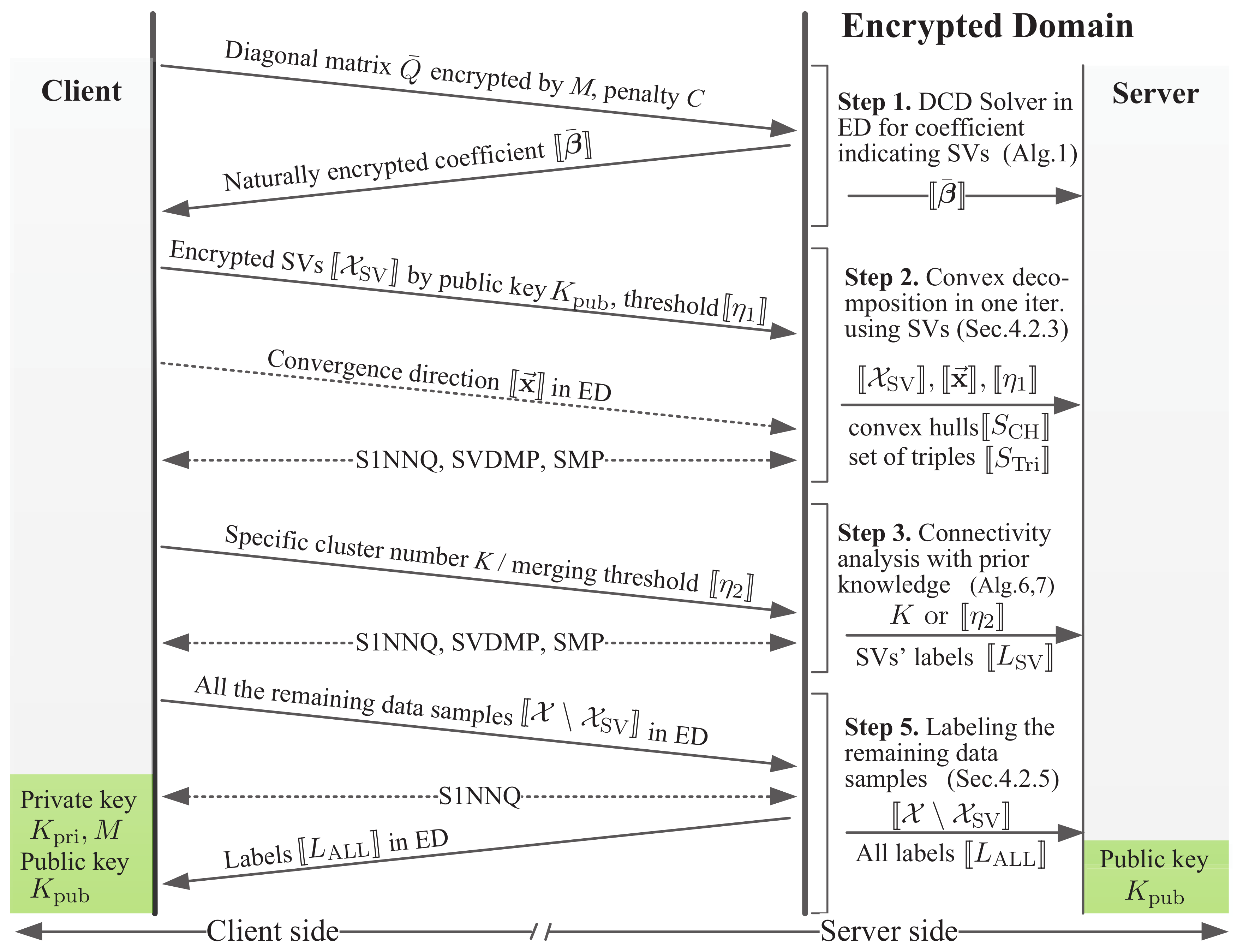
For the second step, the major works are carried out on the client side as a response to the server. As marked in Figure 3, the accessible sensitive data are $\left[\left[{\mathcal{X}}_{\mathrm{SV}}\right]\right]$, $\left[\left[\overrightarrow{\mathbf{x}}\right]\right]$, $\left[\left[{\eta }_1\right]\right]$, $\left[\left[S_{\mathrm{CH}}\right]\right]$ and $\left[\left[S_{\mathrm{Tri}}\right]\right]$. However, all of them are encrypted by $K_{\mathrm{pub}}$.

(3)

Step 3 depends on the output of Step 2. It includes SMP, SCP, and SVDMP whose prototypes are proved by [20]. The server can only get the number of clusters, but cannot infer any relationship between data samples in PD. Furthermore, the client can easily hide the real number by tuning the predefined parameters K or ${\eta }_2$. Then, an uncertain cluster number is meaningless for the server.

(4)

Step 5 employs S1NNQ. The server cannot infer the actual label for a plain data sample, even if it occasionally has several samples.

4.4.4. Security of MPPSVC under the Malicious Model

We extend MPPSVC into a secure protocol under the malicious model where an adversary exists. It may be the server or an eavesdropper. Since the eavesdropper cannot get more information than the server, for simplicity, we only consider the server as an implicit adversary.

For the server, it can arbitrarily deviate from the protocol to gain some advantages (e.g., learning additional information about inputs) over the client. The deviations include, for example, for the server to instantiate MPPSVC with modified queries and to abort the protocol after gaining partial information. Considering SCP, the malicious server might either use a fixed r to obtain the ordering of encrypted numerical values or tamper the two compared numerical values. For the prior, the immediate order for N ciphertext is meaningless for recovering their plaintext, because of ${\mathcal{Z}}_N\subset {\mathcal{Z}}_{n^2}$ and $N\ll n^2$ in bit. For the latter, without $K_{\mathrm{pri}}$, any modification of ciphertext might cause a significant change of its plaintext. The client can easily discover it. Therefore, all the intermediate results are either random or pseudo-random values. Even though an adversary modifies the intermediate computations, he cannot gain any additional information. The modification may eventually result in the wrong output. Thus, if we ensure all the calculations performed and messages sent by the client are correct, the proposed MPPSVC is secure. It provides the ability to validate the server’s works to the client.

5. Experimental Results

5.1. Experimental Setup

In the premise of security for outsourcing, we demonstrated the performance of RSVC-EO in PD and MPPSVC in ED. RSVC-EO dominated the validity while MPPSVC supplied the secure outsourcing framework. Deservedly, we first evaluated the validity and performance of RSVC-EO, and then the performance of MPPSVC.

In PD, the first experiment was to estimate the sensitivity concerning ${\eta }_1$ on accuracy. Since RSVC-EO is designed for local use, its declared advantage is the flexibility of using the pre-computed kernel matrix or not. The second experiment was to check the performance related to kernel utilization. Then, the third series of the benchmark was to give full comparisons of RSVC-EO and the state-of-the-art methods. Besides, we verified the effectiveness of capturing data distribution by all the compared methods regarding the discovered cluster number. In ED, eventually, our primary focuses were the changes in accuracy and efficiency brought by MPPSVC. In this study, the adjusted rand index (ARI) [4,30] was adopted for accuracy evaluation. It is a widely used similarity measure between two data partitions where both true labels and predicted cluster labels are given. Let $N_{ij}$ be the number of data samples with true label i yet assigned by j. $N_{i·}$ and $N_{·j}$ are, respectively, the number of data samples with label i and j. ARI is formulated by

$$\mathrm{ARI}=\frac{{\sum }_{i,j}\left(\genfrac{}{}{0pt}{}{N_{ij}}{2}\right)-\left[{\sum }_i\left(\genfrac{}{}{0pt}{}{n_{i·}}{2}\right){\sum }_j\left(\genfrac{}{}{0pt}{}{N_{·j}}{2}\right)\right]/\left(\genfrac{}{}{0pt}{}{N}{2}\right)}{\frac{1}{2}\left[{\sum }_i\left(\genfrac{}{}{0pt}{}{N_{i·}}{2}\right)+{\sum }_j\left(\genfrac{}{}{0pt}{}{N_{·j}}{2}\right)\right]-\left[{\sum }_i\left(\genfrac{}{}{0pt}{}{N_{i·}}{2}\right){\sum }_j\left(\genfrac{}{}{0pt}{}{N_{·j}}{2}\right)\right]/\left(\genfrac{}{}{0pt}{}{N}{2}\right)}.$$

(17)

5.2. Experimental Dataset

Table 2. Description of the benchmark datasets.

Datasets	Dataset Description
	Dims	Size	# of Classes
wisconsin	9	683	2
glass	9	214	7
wine	13	178	3
movement_libras (mLibras)	90	360	15
P2P traffic (P2P-T)	4	9206	4
WebKB	4	4199	4
abalone	7	4177	29
Reuters-21578(Reuters)	10	9990	10
Ohsumed (Oh)	23	13,929	23
20Newsgroups (20NG)	20	13,998	20
shuttle (sh)	9	43,500	7
kddcup99	9	494,021	5

shows the statistical information of the employed twelve datasets. Here, wisconsin, glass, wine, movement_libras, abalone, and shuttle (training version) were from UCI repository [31]. Four text corpora were employed after a pre-processing, namely ${\mathrm{DC}}_{\mathrm{GLI}}-\mathrm{CCE}$ by Ping et al. [32], i.e., four categories of WebKB [33], full twenty categories of 20Newsgroups [34], top 10 largest categories of Reuters-21578 [35], and Ohsumed with 23 classes [36]. P2P traffic is a collection of 9206 flows’ features that were extracted from traffic supplied by [37] following the method of Peng et al. [38]. Following the work of Guo et al. [39], kddcup99 is a nine-dimensional dataset extracted from KDD Cup 1999 Data [40], which was used to build a network intrusion detector. Due to space limitation, thereafter, we use abbreviations in brackets for dataset with long name.

5.3. Experiments in the Plain-Domain

For local use, RSVC-EO in PD means the data owner frequently cannot have sufficient memory for the required kernel matrix. Consequently, the testbed was a laptop with Intel Dual Core 2.66 GHz and 3 GB available RAM, which calculates kernel function on demand. RSVC-EO and all the other compared methods were implemented and fairly evaluated by MATLAB 2016a on Windows 7-X64.

5.3.1. Analysis of Parameter Sensitivity

Algorithm 2 introduces ${\eta }_1$ to indicate the convex decomposition which might be directly related to RSVC-EO’s performance. Figure 4 depicts the ARI variations achieved by RSVC-EO with respect to ${\eta }_1\in [-0.8,0.9]$ with step $0.01$. Here, variation for each dataset is represented by the rectangle in which the square block is the mean value. Apparently, the variations is very small for 9 out of 12 datasets, i.e., wisconsin, glass, mLibras, P2P-T, WebKB, abalone, Reuters, Oh, and kddcup99. In fact, these variations are lower than $3.21\times {10}^{-4}$. For the other three datasets, i.e., wine, 20NG, and sh, the variations are lower than $5.5\times {10}^{-3}$, and the rectangles’ locations show that most of them are close to the peak value. Therefore, parameter selection of ${\eta }_1$ is frequently an easy work for the proposed RSVC-EO to achieve a relatively optimal clustering result. Notice that a preset ${\eta }_1$ is not required for those cases with prior knowledge of the cluster number K, because RSVC-EO can merge convex hulls until the expected K is obtained.

5.3.2. Analysis of Iteration Sensitivity

The iterative analysis is essential for both RSVC-EO and MPPSVC. Although the server conducts the solver independently to get the encrypted coefficient vector $M\overline{\mathit{\beta }}$, runtime might be pricey if we have to choose the strategy of immediately calculating kernel function for large-scale data. Therefore, we concern whether massive iterations are unavoidable. Noticeably, Hsieh et al. [41] proved that the general DCD solver reaches an $ϵ$-accurate solution in $O(log(1/ϵ\left)\right)$ iterations. For the sake of simplicity, we checked the relationship between the achieved ARI and iteration number in PD. Figure 5 depicts the results where kddcup99 is omitted due to pricey runtime with great iteration number.

For most of the cases, the achieved ARIs are relatively stable, along with the iteration number increases. By employing the proposed solver, a useful phenomenon is that, for each case, the best ARI is usually reached with a small iteration number (≤4). It means that a more precise objective function value of the problem in Equation (2) is not always required in practice. Therefore, a small iteration number meets the requirements from both RSVC-EO and MPPSVC for expected results. This will not bring noticeable computation load to either side.

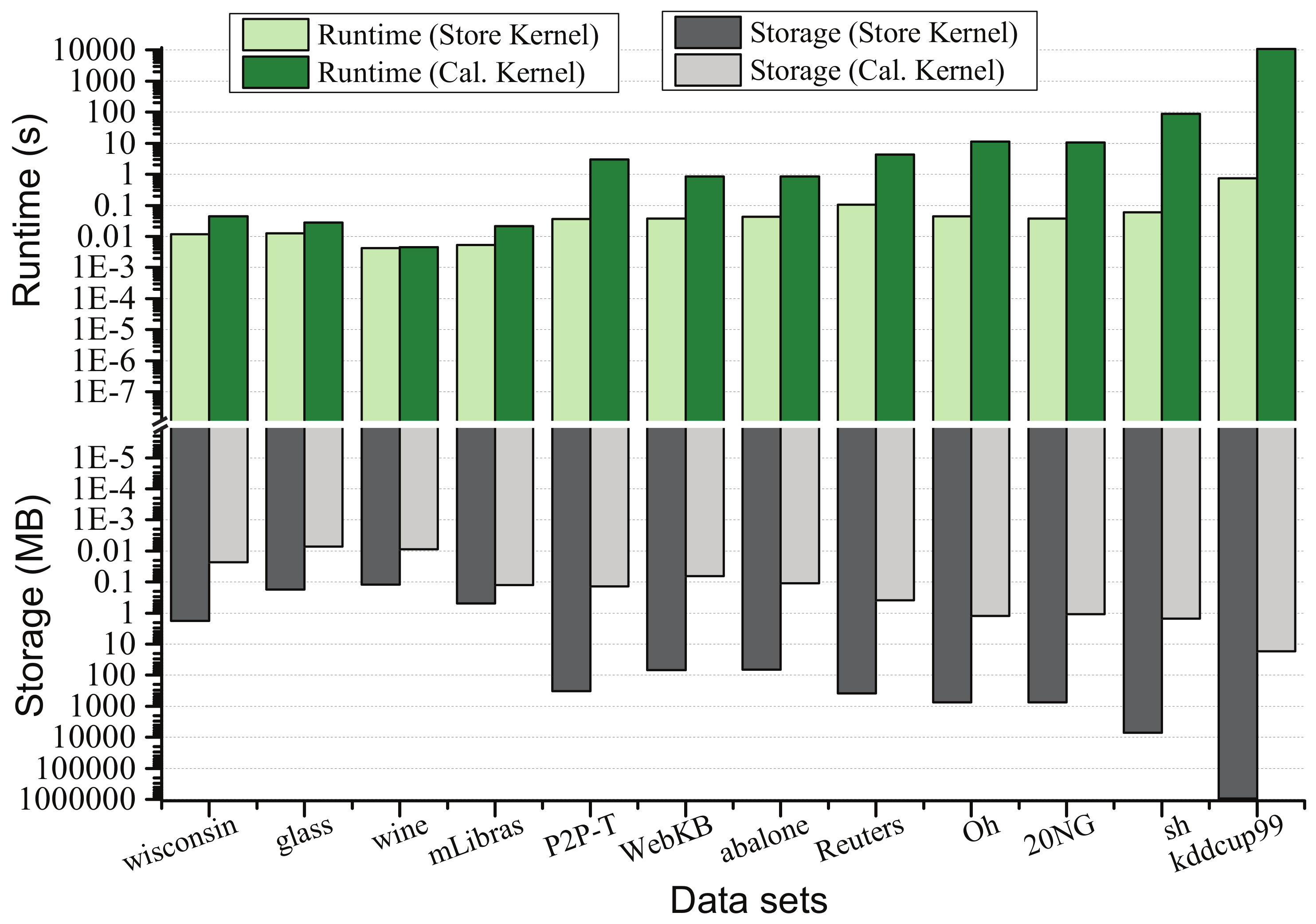
5.3.3. Performance Related to Kernel Utilization

In this section, we check whether RSVC-EO is flexible to balance the efficiency and usability with limited memory. For efficiency, the runtime of completing Algorithm 1 with the pre-computed kernel matrix and with immediate calculating kernel function on Line 5 were separately evaluated. The former is denoted by “Runtime (Store Kernel)” while the latter is “Runtime (Cal. Kernel)”. Meanwhile, their memory consumptions are also evaluated, respectively, as “Storage (Store Kernel)” and “Storage (Cal. Kernel)” (Due to the limited memory (3GB); in fact, the client cannot afford all the experimental datasets’ requirements. Thus, “Runtime (Store Kernel)” for storage exceeding the supplement was estimated by “Runtime (Cal. Kernel)” minus the runtime of calculating $K({\mathbf{x}}_j,{\mathbf{x}}_i)$.). Figure 6 shows the results. Apparently, for small datasets with $N<1000$ such as wisconsin, glass, and wine, there are no obvious differences between “Runtime (Store Kernel)” and “Runtime (Cal. Kernel)”. Although the client affords large dataset analysis well, its “Runtime (Cal. Kernel)” quickly raises as N increases. On the contrary, based on the immediate calculating kernel function, “Runtime (Cal. Kernel)” is linear to the data size, whereas “Storage (Store Kernel)” easily exceeds the client’s capability. Gaps become significantly for those datasets with $N\gg d$. For instance, to deal with sh, the requirement is 7.05 GB for “Storage (Store Kernel)” while “Runtime (Cal. Kernel)’ only needs 1.49 MB. Therefore, efficiency and storage consumptions are strongly related to the kernel utilization. It is critical to outsource the cluster analysis for those resource-limited clients.

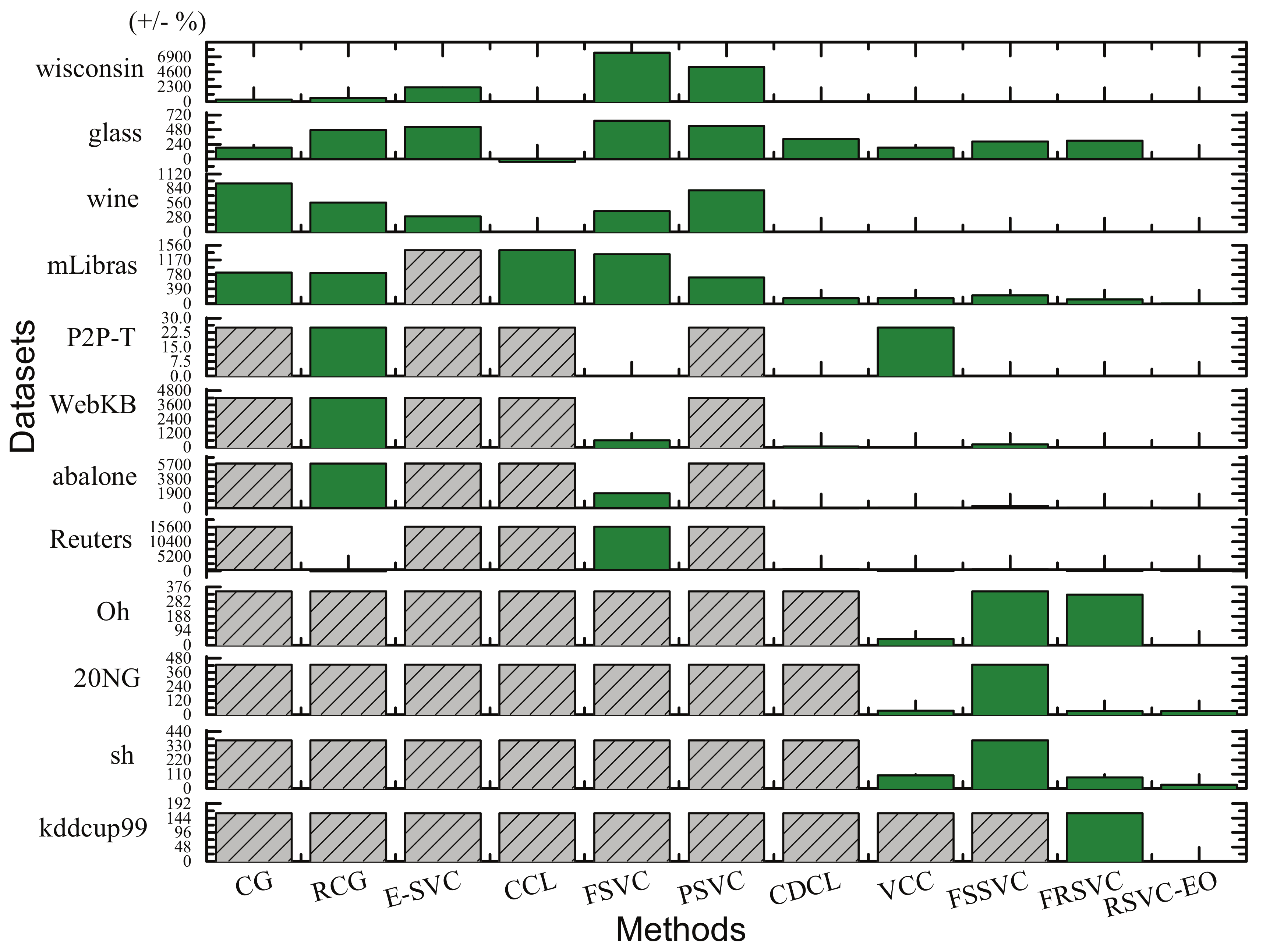
5.3.4. Benchmark Results for Accuracy Comparison

To check RSVC-EO’s performance, we compared it with the state-of-the-art methods: the complete graph (CG) [1], the reduced complete graph (RCG) [24], the equilibrium based SVC (E-SVC) [29,42], the cone cluster labeling (CCL) [43], the fast SVC (FSVC) [12], the position regularized SVC (PSVC) [44], the convex decomposition cluster labeling (CDCL) [23], the voronoi cell-based clustering (VCC) [8], the fast and scalable SVC (FSSVC) [26], and the faster and reformulated SVC (FRSVC) [22].

Table 3. Accuracies (ARI) achieved by the state-of-the-art methods on 12 datasets.

Dataset	CG	RCG	E-SVC	CCL	FSVC	PSVC	CDCL	VCC	FSSVC	FRSVC	RSVC-EO
wisconsin	0.7793	0.8035	0.1344	0.9076	0.6687	0.2574	0.8685	0.8029 ± 0.0514	0.9248	0.8798	0.8632
glass	0.2771	0.2823	0.2743	0.2201	0.2458	0.2801	0.2911	0.2771 ± 0.0031	0.2998	0.2582	0.3540
wine	0.5912	0.7928	0.4159	0.8190	0.8042	0.3809	0.8961	0.8088 ± 0.0563	0.8992	0.8483	0.8185
mLibras	0.2422	0.2356	—	0.0899	0.1421	0.2541	0.3320	0.3065 ± 0.0181	0.3703	0.3366	0.3732
P2P-T	—	0.8815	—	—	0.8367	—	0.8917	0.7389 ± 0.0066	0.8815	0.8678	0.8807
WebKB	—	0.3072	—	—	0.5144	—	0.4645	0.4434 ± 0.0156	0.5670	0.6395	0.5381
abalone	—	0.0332	—	—	0.0515	—	0.0603	0.0710 ± 0.0011	0.0587	0.0657	0.0996
Reuters	—	0.0148	—	—	0.4775	—	0.8064	0.4908 ± 0.0616	0.5831	0.7295	0.8338
Oh	—	—	—	—	—	—	—	0.4280 ± 0.0292	0.4514	0.4840	0.5019
20NG	—	—	—	—	—	—	—	0.4397 ± 0.0461	0.3628	0.4927	0.6084
sh	—	—	0.59 [12]	—	0.58 [12]	—	—	0.5898 ± 0.0198	0.6857	0.8050	0.7337
kddcup99	—	—	—	—	—	—	—	—	—	—	0.7621

Note: “—” means not available due to insufficient memory or too much time consumption.

gives the achieved accuracies regarding ARI, and the corresponding runtime of the training phase and the labeling phase for each dataset is illustrated in Figure 7. Three points are important to be noted. First, due to the sampling strategy, VCC cannot achieve a fixed accuracy even though its parameters are fixed. We use its mean and mean-square deviation of the top ten ARIs. Secondly, runtime for each dataset is the average time of ten executions. Thirdly, not all methods can finish analysis on the client while the kernel matrix is too large or too much time (≥4 h. in this study) required by any phase. For these cases, we use “—” to denote an unavailable ARI and mark the runtime with 0. Meanwhile, we collect runtime of FRSVC and RSVC-EO by adopting the immediate calculation of kernel function.

In Table 3, the first rank is highlighted by boldface. Apparently, RSVC-EO reaches the best performance on 7 out of 12 datasets, especially for the large ones such as Reuters, Oh, 20NG, and kddcup99, whereas FRSVC performs better on sh and WebKB, FSSVC outperforms the others on wine and wisconsin, and CDCL gets better results on P2P-T. As data size increases, many traditional methods cannot run well on our client, e.g., CG, E-SVC, CCL, and PSVC. We directly quoted the results of E-SVC and FSVC on sh in [12]. Additionally, RSVC-EO frequently gets into the first three ranks in the other cases, e.g. sh, WebKB, and P2P-T. Thus, regarding the accuracy, we guess that RSVC-EO is suitable for relatively large datasets. To verify it, we also give the results of pair comparison in

Table 4. Comparison under non-parametric statistical test.

Methods	Average Ranks	Unadjusted p	${\mathit{p}}_{\mathbf{Homm}}$
Control Method: RSVC-EO, Average Rank = 2.1667
CG	8.3333	5.2539 $\times {10}^{-6}$	4.2031 $\times {10}^{-5}$
RCG	6.7500	7.1174 $\times {10}^{-4}$	0.0036
E-SVC	8.7083	1.3562 $\times {10}^{-6}$	1.3562 $\times {10}^{-5}$
CCL	8.0417	1.4315 $\times {10}^{-5}$	1.0020 $\times {10}^{-4}$
FSVC	7.1250	2.5028 $\times {10}^{-4}$	0.0015
PSVC	8.4583	3.3728 $\times {10}^{-6}$	2.6982 $\times {10}^{-5}$
CDCL	4.6250	0.0694	0.2083
VCC	5.5000	0.0138	0.0553
FSSVC	2.9167	0.5796	0.5796
FRSVC	3.3749	0.3722	0.5796

following the work of Garcia and Herrera [45]. Here, RSVC-EO is the control method. A nonparametric statistical test, namely Friedman test, was employed to get the average ranks and unadjusted p values. By introducing an adjustment method, Bergmann–Hommel procedure, the adjusted p-value denoted by $p_{\mathrm{Homm}}$ corresponding to each comparison was obtained. RSVC-EO reaches the best performance in the view of average rank. Since the Bergmann–Hommel procedure rejects those hypotheses with p-values $\le 0.016$, together with the values of $p_{\mathrm{Homm}}$, we further confirm RSVC-EO’s better performance.

In Figure 7, some obvious observations for the training phase can be found. (1) For the cases smaller than WebKB, most of the methods perform similarly, including FRSVC and RSVC-EO. Although they have to calculate the kernel function, this might be balanced due to more iterations for the others. However, CCL and PSVC still consume a lot for strict restrictions. CCL requires more iterative analysis to guarantee $R<1$, while PSVC needs a pre-analysis to determine the weight for each data sample and imposes these weights as additional constraints. (2) Along with data size increases, e.g., from WebKB to Reuters, runtime for most of the methods raises dramatically. Particularly, CG, E-SVC, CCL, and PSVC want memory greater than the predefined upper bound. When the kernel matrix requires memory getting close to or greater than the client’s supplement, such as Oh, 20NG, and sh, only two groups of methods are valid. The first group includes VCC (sample rate $\theta \in [0.001,0.5)$) and FSSVC, which adopts sampling strategy. Together with accuracies in Table 3, FSSVC obtains better accuracy and consumes much more memory because of steadily choosing boundaries, whereas VCC prefers a random strategy. The second group consists of FRSVC and RSVC-EO, which calculate the kernel function on demand to avoid huge memory consumption. Despite having greater runtime than VCC, they are rewarded with better accuracies. A remarkable finding is that benefited by better performance of the parameter insensitivity; fewer iterations required by RSVC-EO’s learning lead to less runtime requirement. (3) For kddcup99, the full kernel matrix with approximate size $2.44\times {10}^{11}$ wants 909.18 GB, which is far greater than what the client can afford. VCC and FSSVC fail because they can hardly select appropriate data samples to describe the pattern, while FRSVC fails for pricey labeling strategy. Only RSVC-EO finishes the analysis with a suboptimal result because we only use one iteration in Algorithm 1. Therefore, there still will be a big challenge for RSVC-EO to obtain the optimal result when the data size continues to increase.

For the labeling phase, RSVC-EO outperforms the others significantly that confirms the core ideas of FCDCL. Firstly, FCDCL does not use iterative analysis. Thus, it performs well on high-dimensional data, such as mLibras and Oh, whereas ESVC fails and the others consume much more. Secondly, connectivity analysis of FCDCL avoids the traditional sampling checks in feature space. It reduces the impact of candidate sample pairs. Although the others try to reduce the number of sample pairs and the sample rate, runtime for the essential sample analysis is longer than the proportional time to the size of the dataset or the candidate subset.

5.3.5. Effectiveness of Capturing Data Distribution

Following Xu and Wunsch [30], we find that increasing the cluster number sometimes has a positive impact on the accuracy measures. However, we should try to avoid splitting data samples of a group into multiple clusters. We intuitively expect an effective method which can accurately capture data distribution. Therefore, we use the difference between the captured cluster number $N_{\mathrm{C}}$ and the real number of classes $N_{\mathrm{R}}$ summarized in Table 2, in terms of percentage $(\frac{N_{\mathrm{C}}}{N_{\mathrm{R}}}-1)\times 100\%$. Comparisons amongst the eleven methods are illustrated by Figure 8. If a method is invalid on a dataset, the corresponding percentage is assigned by the greatest value amongst the other finished ones, and its column is gray with slashes. Certainly, the shorter the column for a dataset is, the better effect the corresponding method performs. As shown in Figure 8, RSVC-EO outperforms the other ten methods significantly.

5.4. Experiments in the Encrypted-Domain

To integrate the Paillier, MPPSVC was implemented by C++ using GNU GMP library version 6.0.0a (https://ftp.gnu.org/gnu/gmp/).Both the server and the client were modeled as different threads of a single program, which passes data or parameters to each other following the rules shown in Figure 3. We conducted experiments on a server with Quad-Core $2.29$ GHz CPUs and 64 GB main memory running on Windows 7-X64.

5.4.1. Performance in the Encrypted-Domain

In ED, the Paillier only allows integers. We introduce a scaling factor $\gamma$ on the input data samples and the exchanged data to take integers downwardly before encryption.

Table 5. ARIs achieved in ED for various scaling factor $\gamma$.

Dataset	Scaling Factor $\mathit{\gamma }$
	${\mathbf{10}}^{\mathbf{1}}$	${\mathbf{10}}^{\mathbf{2}}$	${\mathbf{10}}^{\mathbf{3}}$	${\mathbf{10}}^{\mathbf{4}}$	${\mathbf{10}}^{\mathbf{5}}$
wisconsin	0.8254	0.8519	0.8519	0.8519	0.8519
glass	0.1817	0.3197	0.3540	0.3540	0.3540
wine	0.4272	0.8185	0.8185	0.8185	0.8185
mLibras	0.3281	0.3264	0.3415	0.3415	0.3415
P2P-T	0.7757	0.7938	0.8048	0.8048	0.8048
WebKB	0.4824	0.5235	0.4428	0.4795	0.4795
abalone	0.0870	0.0915	0.0917	0.0917	0.0917
Reuters	0.7860	0.7284	0.7063	0.7062	0.7062
Oh	0.4851	0.4954	0.4898	0.4898	0.4898
20NG	0.4752	0.5120	0.5171	0.5169	0.5169
sh	0.6586	0.6346	0.6346	0.6596	0.6596
kddcup99	0.6799	0.7629	0.7714	0.7620	0.7620

shows the accuracies for various $\gamma$ in ED. Although better accuracies are not always obtained with greater $\gamma$, the clustering results (marked by underlines) become steadily when $\gamma$ is above ${10}^4$. For these cases, the accuracies are either the best ones (highlighted by boldface) or very close to the best. Hence, four decimal points are sufficient for the 12 datasets. Compared with Table 3, we find that $\gamma$ has little influence on accuracy in ED because both the input data samples and the intermediate results transmitted from the client to the server might lose a certain degree of precision. Since the accuracies achieved by MPPSVC are very close to those obtained by RSVC-EO in PD, we confirm the guaranteed privacy of the input data and clustering procedure.

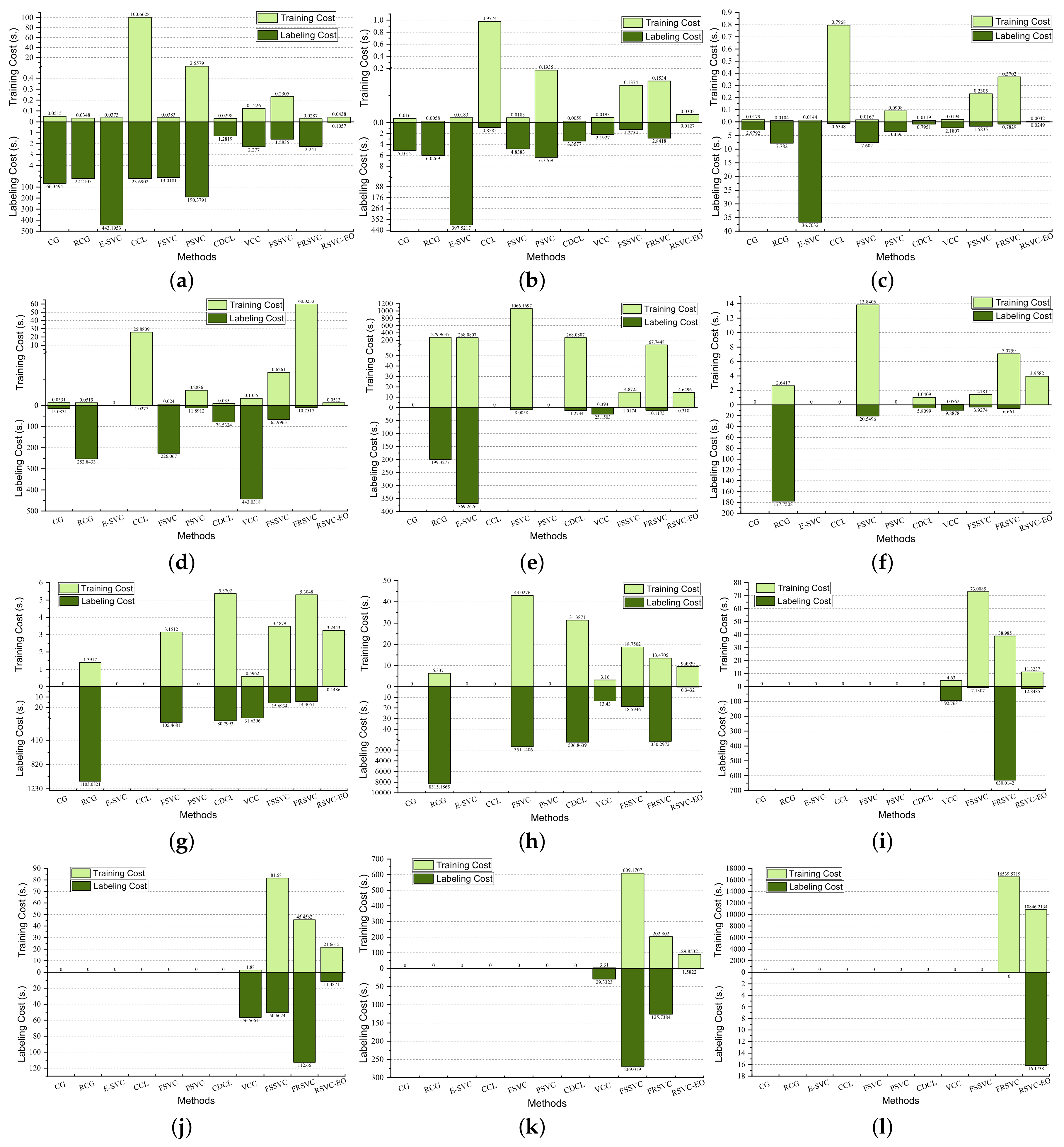
5.4.2. Computational Complexity

Table 6. Runtime (s) of each step in ED, respectively, consumed by the client (C) and the server (S).

Dataset	Step 1		Step 2		Step 3		Step 5		#SVs	#Convex Hulls
	C	S	C	S	C	S	C	S
wisconsin	1.2524	0.0194	21.6361	43.4891	1.3200	9.4463	0.0200	1.4403	64	30
glass	0.7072	0.0059	14.4307	22.4403	1.2900	9.4809	0.0164	1.3288	44	31
wine	1.1567	0.0567	24.8310	40.4476	1.8900	21.4400	0.0244	3.0628	51	43
mLibras	4.3020	0.0186	195.1682	305.3468	0.8100	67.2533	0.0713	12.9299	62	23
P2P-T	4.6369	0.0805	103.4480	1577.1325	21.1350	356.6295	0.0112	8.0530	661	471
WebKB	0.7981	0.0057	41.7010	267.3922	6.1050	37.9054	0.0031	2.7794	266	137
abalone	0.9594	0.0131	49.0764	225.5012	2.6700	17.8104	0.0052	2.9876	189	69
Reuters	0.5403	0.0148	27.2192	59.0562	0.5250	4.5836	0.0081	1.4473	75	15
Oh	1.9096	0.0171	93.8732	255.4895	1.1250	18.1687	0.0175	4.8598	113	25
20NG	0.8993	0.0140	45.5341	77.9957	0.8250	16.2751	0.0152	2.8590	63	25
sh	1.4285	0.0259	45.9365	166.4430	0.8550	6.2177	0.0103	2.3485	141	22
kddcup99	0.4751	1.3404	24.8795	54.2872	0.6900	4.7367	0.0068	1.3015	74	17

Note: Step 5 can classify all the arrival data one by one or in parallel, and we collect the consumptions for a single sample for efficiency analysis.

presents the runtime of each step (following Table 1) in ED consumed, respectively, by the client and the server. “#SVs” and “#Convex Hulls”, respectively, denote the number of SVs and convex hulls. We omit the consumption of outsourcing the pre-computation for M following Luo et al. [27] because it is not in the proposed framework.

Together with Figure 7, we can make several observations. (1) Step 1 is no longer the first barrier for the client even though the solver requires a large number of iterations. For example, in Figure 7l, Step 1 for kddcup99 still consumes 10,846.2134 s although we cut off the iterations to get the suboptimal result for efficiency. Now, it only requires 0.4751 s by the client without considering the iterations on the server. (2) Step 2 is the most time-consumption task for both sides, and Step 3 takes the second place. Comparing the first two time-consuming datasets P2P-T and mLibras with the others, efficiency is closely related to “#SVs” and “#Convex Hulls”. From Definition 2, “#SVs” also affects “#Convex Hulls”. Since S1NNQ compares each unlabeled data sample with both SVs and density centroids, “#SVs” and “#Convex Hulls” directly contribute the computational time of Step 5. (3) Dimensionality is another critical factor. The evidence can be found on the small data mLibras with 90 dimensions. Since each dimension should be encrypted/decrypted separately, high dimensionality increases the computational time in ED and results in more SVs. (4) Similar to the method in [17], Step 5 is a classification work in ED, which can be conducted one by one or in parallel. It is a light workload to outsource the encrypted sample for its label. (5) The total time cost is proportional to data size yet in an acceptable range for the client. However, we do not suggest outsourcing Steps 1–3 for small data analysis due to the increased costs. Based on a learned model, Step 5 is also suitable for being outsourced as a service.

6. Related Work

Despite handling arbitrary cluster shapes well, SVC suffers from pricey computation and memory as data size increases. Generally, exploring ways of optimizing the critical operations and asking for the Cloud’s help are potential countermeasures. For the former way, the training and labeling phases are considered, respectively.

(1)

For model training, the core is solving the dual problem in Equation (2). Major studies prefer generic optimization algorithms, e.g., gradient descent, sequential minimal optimization [4], and evolutionary strategies [46]. Later, studies rewrote the dual problem by introducing the Jaynes maximum entropy [47], the position-based weight [44], and the relationship amongst SVs [26]. However, conducting a solver with the full dataset suffers from huge consumption of kernel matrix. Thus, FSSVC [26] steadily selects the boundaries while VCC [8] samples a predefined ratio $\theta \in (0,1]$ of data. Other methods related to reducing the working set and divide-and-conquer strategy were surveyed in [4]. However, bottlenecks still easily appear due to the nonlinear strategy and the pre-computed kernel matrix. Thus, FRSVC [22] employs a linear method to seek a balance between efficiency and memory cost.

(2)

For the labeling phase, connectivity analysis adopts a sampling check strategy for a long time. Reducing the number of sample pairs thus becomes the first consideration, for instance, using the full dataset by CG [1], the SVs by PSVC [44], the SEVs by RCG [24], and the transition points by E-SVC [29,42]. Although the number of sample pairs is gradually reduced, they have a side-effect of additional iterations in seeking SEVs or TS. Thus, CDCL [23] suggests a compromise way of using SVs to construct convex hulls, which are employed as substitutes of SEVs. For efficiency, CDCL reduces the average sample rate by a nonlinear sampling strategy. Later, FSSVC [26] and FRSVC [22] made further improvements by reducing the average sample m close to 1. Besides, Chiang and Hao [48] introduced a cell growth strategy, which starts at any data sphere, expands by absorbing fresh neighboring spheres, and splits if its density is reduced to a certain degree. Later, CCL [43] created a new way by checking the connectivity of two SVs according to a single distance calculation. However, too strict constraints emphasized on the solver degrade its performance. In fact, for these methods, the other pricey consumption is the adjacent matrix, which usually ranges from $O\left(N_{\mathrm{SV}}^2\right)$ to $O\left(N^2\right)$.

As data size increases, pricey computation and huge space needed by the above solutions raise the requirement of outsourcing. However, to ask for the Cloud’s help, the risk of data leakage raises concerns, since both the input data and the learned model memorize information [10]. The major studies focus on securely outsourcing known SVM classifiers. Generally, the secure outsourcing protocols prefer introducing homomorphic encryption [15,16,17,49], reformulating the classifier [50], randomizing the classifier [51], or finding an approximated classifier [21]. Furthermore, based on the homomorphic encryption, the existing secure outsourcing methods support the calculation of rational numbers [52], matrix computations [14,27,28], mathematical optimization [14], and k nearest neighboring query [20]. However, very few works are related to privacy-preserving model training. An early work was published by Lin et al. [19], who suggested a random linear transformation for data’s subset before outsourcing. Later, Salinas et al. [53] presented a transformed quadratic program and its solver, namely Gauss–Seidel algorithm, for securely outsourcing SVM training while reducing the client’s computation. According to a primal estimated sub-gradient solver and replacing the SVs with data prototypes, the most recent work [54] gives a solution of training SVM model with data encrypted by homomorphic encryption.

In a sense, training an SVM model and making a decision for a data sample is similar to the training phase and the last labeling step, respectively. However, the known solutions are not suitable for SVC due to the distinguished iteration/analysis strategy and operations in feature space. To the best of our knowledge, no practical solution is presented for secure outsourcing SVC despite strong demand.

7. Conclusions and Future Work

Towards easing the client’s workload, we propose MPPSVC to make all the phases of SVC outsourceable without worrying about privacy issues. For simplicity and generality, we suggest using additively homomorphic encryption to protect data privacy. The limited operations motivate us giving a new design of RSVC-EO based on elementary operations. However, inevitable iterations for Equation (2) and complex computations in all phases of SVC may cause massive interactions. For efficiency, we consequently protect the kernel by a matrix transformation, which not only reduces data transmission but also makes the outsourced solver iterate well. Besides, for the labeling phase of RSVC-EO, FCDCL is developed without iterative analysis. Taking RSVC-EO as the core, MPPSVC consists of several customized, lightweight, and secure protocols. Theoretical analysis and experimental results on twelve datasets prove the reliability of the proposed methods, i.e., RSVC-EO for local use and MPPSVC for outsourcing.

Although MPPSVC provides customizable phase outsourcing, security and efficiency are ever-lasting issues, which should be balanced as data size increases. How to securely control the iterations while reducing SVs, finding substitutes for the complex operations, avoiding unnecessary kernel matrix consumption, and making full use of distributed computing are worthy of investigation.

References

1. Ben-Hur, A.; Horn, D.; Siegelmann, H.T.; Vapnik, V.N. Support Vector Clustering. J. Mach. Learn. Res. 2001, 2, 125–137. [Google Scholar] [CrossRef]
2. Saltos, R.; Weber, R.; Maldonado, S. Dynamic Rough-Fuzzy Support Vector Clustering. IEEE Trans. Fuzzy Syst. 2017, 25, 1508–1521. [Google Scholar] [CrossRef]
3. Ye, Q.; Zhao, H.; Li, Z.; Yang, X.; Gao, S.; Yin, T.; Ye, N. L1-Norm Distance Minimization-Based Fast Robust Twin Support Vector k-Plane Clustering. IEEE Trans. Neural Netw. Learn. Syst. 2018, 29, 4494–4503. [Google Scholar] [CrossRef] [PubMed]
4. Li, H.; Ping, Y. Recent Advances in Support Vector Clustering: Theory and Applications. Int. J. Pattern Recogn. Artif. Intell. 2015, 29, 1550002. [Google Scholar] [CrossRef]
5. Sheng, Y.; Hou, C.; Si, W. Extract Pulse Clustering in Radar Signal Sorting. In Proceedings of the 2017 International Applied Computational Electromagnetics Society Symposium–Italy (ACES), Florence, Italy, 26–30 March 2017; pp. 1–2. [Google Scholar]
6. Lawal, I.A.; Poiesi, F.; Anguita, D.; Cavallaro, A. Support Vector Motion Clustering. IEEE Trans. Circuits Syst. Video Technol. 2017, 27, 2395–2408. [Google Scholar] [CrossRef]
7. Pham, T.; Le, T.; Dang, H. Scalable Support Vector Clustering Using Budget. arXiv 2017, arXiv:1709.06444v1. [Google Scholar]
8. Kim, K.; Son, Y.; Lee, J. Voronoi Cell-Based Clustering Using a Kernel Support. IEEE Trans. Knowl. Data Eng. 2015, 27, 1146–1156. [Google Scholar] [CrossRef]
9. Yu, Y.; Li, H.; Chen, R.; Zhao, Y.; Yang, H.; Du, X. Enabling Secure Intelligent Network with Cloud-Assisted Privacy-Preserving Machine Learning. IEEE Netw. 2019, 33, 82–87. [Google Scholar] [CrossRef]
10. Song, C.; Ristenpart, T.; Shmatikov, V. Machine Learning Models that Remember Too Much. In Proceedings of the 2017 ACM SIGSAC Conference on Computer and Communications Security, CCS’ 2017, Dallas, TX, USA, 30 October–3 November 2017; ACM: New York, NY, USA, 2017; pp. 587–601. [Google Scholar]
11. Dritsas, E.; Kanavos, A.; Trigka, M.; Sioutas, S.; Tsakalidis, A. Storage Efficient Trajectory Clustering and k-NN for Robust Privacy Preserving Spatio-Temporal Databases. Algorithms 2019, 12, 266. [Google Scholar] [CrossRef] [Green Version]
12. Jung, K.H.; Lee, D.; Lee, J. Fast support-based clustering method for large-scale problems. Pattern Recogn. 2010, 43, 1975–1983. [Google Scholar] [CrossRef]
13. Paillier, P. Public-Key Cryptosystems Based on Composite Degree Residuosity Classes. In Proceedings of the 17th International Conference on Theory and Application of Cryptographic Techniques (EUROCRYPT’ 99), Prague, Czech Republic, 2–6 May 1999; pp. 223–238. [Google Scholar]
14. Shan, Z.; Ren, K.; Blanton, M.; Wang, C. Practical Secure Computation Outsourcing: A Survey. ACM Comput. Surv. 2018, 51, 31:1–31:40. [Google Scholar] [CrossRef]
15. Liu, X.; Deng, R.; Choo, K.R.; Yang, Y. Privacy-Preserving Outsourced Support Vector Machine Design for Secure Drug Discovery. IEEE Trans. Cloud Comput. 2019, 1–14. [Google Scholar] [CrossRef]
16. Rahulamathavan, Y.; Veluru, S.; Phan, R.C.W.; Chambers, J.A.; Rajarajan, M. Privacy-Preserving Clinical Decision Support System using Gaussian Kernel based Classification. IEEE J. Biomed. Health Inform. 2014, 18, 56–66. [Google Scholar] [CrossRef] [PubMed] [Green Version]
17. Rahulamathavan, Y.; Phan, R.C.W.; Veluru, S.; Cumanan, K.; Rajarajan, M. Privacy-Preserving Multi-Class Support Vector Machine for Outsourcing the Data Classification in Cloud. IEEE Trans. Dependable Secure Comput. 2014, 11, 467–479. [Google Scholar] [CrossRef] [Green Version]
18. Karapiperis, D.; Verykios, V.S. An LSH-based Blocking Approach with A Homomorphic Matching Technique for Privacy-preserving Record Linkage. IEEE Trans. Knowl. Data Eng. 2015, 27, 909–921. [Google Scholar] [CrossRef]
19. Lin, K.P.; Chang, Y.W.; Chen, M.S. Secure Support Vector Machines Outsourcing with Random Linear Transformation. Knowl. Inf. Syst. 2015, 44, 147–176. [Google Scholar] [CrossRef]
20. Samanthula, B.; Elmehdwi, Y.; Jiang, W. k-Nearest Neighbor Classification over Semantically Secure Encrypted Relational Data. IEEE Trans. Knowl. Data Eng. 2015, 27, 1261–1273. [Google Scholar] [CrossRef] [Green Version]
21. Lin, K.P.; Chen, M.S. On the Design and Analysis of the Privacy-Preserving SVM Classifier. IEEE Trans. Knowl. Data Eng. 2011, 23, 1704–1717. [Google Scholar] [CrossRef]
22. Ping, Y.; Tian, Y.; Guo, C.; Wang, B.; Yang, Y. FRSVC: Towards making support vector clustering consume less. Pattern Recogn. 2017, 69, 286–298. [Google Scholar] [CrossRef]
23. Ping, Y.; Tian, Y.; Zhou, Y.; Yang, Y. Convex Decomposition Based Cluster Labeling Method for Support Vector Clustering. J. Comput. Sci. Technol. 2012, 27, 428–442. [Google Scholar] [CrossRef]
24. Lee, J.; Lee, D. An Improved Cluster Labeling Method for Support Vector Clustering. IEEE Trans. Pattern Anal. Mach. Intell. 2005, 27, 461–464. [Google Scholar] [PubMed]
25. Ping, Y.; Zhou, Y.; Yang, Y. A Novel Scheme for Accelerating Support Vector Clustering. Comput. Inform. 2011, 31, 1001–1026. [Google Scholar]
26. Ping, Y.; Chang, Y.; Zhou, Y.; Tian, Y.; Yang, Y.; Zhang, Z. Fast and Scalable Support Vector Clustering for Large-scale Data Analysis. Knowl. Inf. Syst. 2015, 43, 281–310. [Google Scholar] [CrossRef]
27. Luo, C.; Zhang, K.; Salinas, S.; Li, P. SecFact: Secure Large-scale QR and LU Factorizations. IEEE Trans. Big Data 2019, 1–13. [Google Scholar] [CrossRef]
28. Zhou, L.; Li, C. Outsourcing Eigen-Decomposition and Singular Value Decomposition of Large Matrix to a Public Cloud. IEEE Access 2016, 4, 869–879. [Google Scholar] [CrossRef]
29. Lee, J.; Lee, D. Dynamic Characterization of Cluster Structures for Robust and Inductive Support Vector Clustering. IEEE Trans. Pattern Anal. Mach. Intell. 2006, 28, 1869–1874. [Google Scholar]
30. Xu, R.; Wunsch, D.C. Clustering; A John Wiley & Sons: Hoboken, NJ, USA, 2008. [Google Scholar]
31. Frank, A.; Asuncion, A. UCI Machine Learning Repository. 2010. Available online: http://archive.ics.uci.edu/ml (accessed on 23 July 2018).
32. Ping, Y.; Zhou, Y.; Xue, C.; Yang, Y. Efficient representation of text with multiple perspectives. J. China Univ. Posts Telecommun. 2012, 19, 101–111. [Google Scholar] [CrossRef]
33. Graven, M.; DiPasquo, D.; Freitag, D.; McCallum, A.; Mitchell, T.; Nigam, K.; Slattery, S. Learning to Extract Symbolic Knowledge form The World Wide Web. In Proceedings of the 15th National Conference for Artificial Intelligence (AAAI’98), Madison, WI, USA, 26–30 July 1998; pp. 509–516. [Google Scholar]
34. Lang, K. NewsWeeder: Learning to filter netnews. In Proceedings of the Twelfth International Conference on Machine Learning, Tahoe City, CA, USA, 9–12 July 1995; pp. 331–339. [Google Scholar]
35. Lewis, D.D. Reuters-21578 Text Categorization Collection. 1997. Available online: http://kdd.ics.uci.edu/databases/reuters21578/ (accessed on 19 March 2012).
36. Hersh, W.R.; Buckley, C.; Leone, T.J.; Hickam, D.H. Ohsumed: An Interactive Retrieval Evaluation and New Large Test Collection for Research. In Proceedings of the 17th Annual ACM SIGIR Conference, Dublin, Ireland, 3–6 July 1994; pp. 192–201. [Google Scholar]
37. UNIBS. The UNIBS Anonymized 2009 Internet Traces. 18 March 2010. Available online: http://www.ing.unibs.it/ntw/tools/traces (accessed on 12 May 2011).
38. Peng, J.; Zhou, Y.; Wang, C.; Yang, Y.; Ping, Y. Early TCP Traffic Classification. J. Appl. Sci.-Electron. Inf. Eng. 2011, 29, 73–77. [Google Scholar]
39. Guo, C.; Zhou, Y.; Ping, Y.; Zhang, Z.; Liu, G.; Yang, Y. A Distance Sum-based Hybrid Method for Intrusion Detection. Appl. Intell. 2014, 40, 178–188. [Google Scholar] [CrossRef]
40. UCI. Kdd Cup 99 Intrusion Detection Dataset. 1999. Available online: http://kdd.ics.uci.edu/databases/kddcup99/kddcup99.html (accessed on 10 February 2016).
41. Hsieh, C.J.; Chang, K.W.; Lin, C.J.; Keerthi, S.S.; Sundararajan, S. A Dual Coordinate Descent Method for Large-scale Linear SVM. In Proceedings of the 25th International Conference on Machine Learning (ICML ’08), Helsinki, Finland, 5–9 July 2008; ACM: New York, NY, USA, 2008; pp. 408–415. [Google Scholar]
42. Lee, D.; Jung, K.H.; Lee, J. Constructing Sparse Kernel Machines Using Attractors. IEEE Trans. Pattern Anal. Mach. Intell. 2009, 20, 721–729. [Google Scholar]
43. Lee, S.H.; Daniels, K.M. Cone Cluster Labeling for Support Vector Clustering. In Proceedings of the 6th SIAM Conference on Data Mining, Bethesda, MD, USA, 20–22 April 2006; pp. 484–488. [Google Scholar]
44. Wang, C.D.; Lai, J.H. Position Regularized Support Vector Domain Description. Pattern Recogn. 2013, 46, 875–884. [Google Scholar] [CrossRef]
45. Garcia, S.; Herrera, F. An Extension on “Statistical Comparisons of Classifiers over Multiple Datasets” for all Pairwise Comparisons. J. Mach. Learn. Res. 2008, 9, 2677–2694. [Google Scholar]
46. Jun, S.H. Improvement of Support Vector Clustering using Evolutionary Programming and Bootstrap. Int. J. Fuzzy Logic Intell. Syst. 2008, 8, 196–201. [Google Scholar] [CrossRef] [Green Version]
47. Guo, C.; Li, F. An Improved Algorithm for Support Vector Clustering based on Maximum Entropy Principle and Kernel Matrix. Expert Syst. Appl. 2011, 38, 8138–8143. [Google Scholar] [CrossRef]
48. Chiang, J.H.; Hao, P.Y. A New Kernel-based Fuzzy Clustering Approach: Support Vector Clustering with Cell Growing. IEEE Trans. Fuzzy Syst. 2003, 11, 518–527. [Google Scholar] [CrossRef]
49. Hua, J.; Shi, G.; Zhu, H.; Wang, F.; Liu, X.; Li, H. CAMPS: Efficient and Privacy-Preserving Medical Primary Diagnosis over Outsourced Cloud. Inf. Sci. 2019. [Google Scholar] [CrossRef]
50. Sumana, M.; Hareesha, K. Modelling A Secure Support Vector Machine Classifier for Private Data. Int. J. Inf. Comput. Secur. 2018, 10, 25–41. [Google Scholar] [CrossRef]
51. Jia, Q.; Guo, L.; Jin, Z.; Fang, Y. Preserving Model Privacy for Machine Learning in Distributed Systems. IEEE Trans. Parallel Distrib. Syst. 2018, 29, 1808–1822. [Google Scholar] [CrossRef]
52. Liu, X.; Choo, K.R.; Deng, R.H.; Lu, R.; Weng, J. Efficient and Privacy-Preserving Outsourced Calculation of Rational Numbers. IEEE Trans. Dependable Secure Comput. 2018, 15, 27–39. [Google Scholar] [CrossRef]
53. Salinas, S.; Luo, C.; Liao, W.; Li, P. Efficient Secure Outsourcing of Large-scale Quadratic Programs. In Proceedings of the ASIA CCS ’16: 11th ACM on Asia Conference on Computer and Communications Security, Xi’an, China, 31 May–3 June 2016; ACM: New York, NY, USA, 2016; pp. 281–292. [Google Scholar]
54. Gonzalez-Serrano, F.J.; Navia-Vazquez, A.; Amor-Martin, A. Training Support Vector Machines with privacy-protected data. Pattern Recogn. 2017, 72, 93–107. [Google Scholar] [CrossRef]
Figure 1. Architecture of secure outsourcing each phase of SVC.
Electronics 09 00178 g001
Figure 2. Diagram for the principles of convex decomposition and connectivity analysis: (a) convex decomposition; and (b) connectivity analysis.
Electronics 09 00178 g002
Figure 3. The flow diagram for approaches of MPPSVC. To keep consistent with Table 1, we use Steps 1, 2, 3, and 5 to denote the four steps of MPPSVC.
Electronics 09 00178 g003
Figure 4. Sensitive analysis by variations of ARI with respect to η 1 [ 0.8 , 0.9 ] with step 0.01 .
Electronics 09 00178 g004
Figure 5. ARIs correspond to different iteration numbers.
Electronics 09 00178 g005
Figure 6. Runtime and storage performance with respect to using kernel utilization or not.
Electronics 09 00178 g006
Figure 7. Runtime comparisons of the training phase and labeling phase for the state-of-the-art methods on 12 datasets: (a) wisconsin; (b) glass; (c) wine; (d) mLibras; (e) P2P-T; (f) WebKB; (g) abalone; (h) Reuters; (i) Oh; (j) 20NG; (k) sh; and (l) kddcup99.
Electronics 09 00178 g007
Figure 8. Difference between the captured cluster number (while each method achieve its best accuracy) and the real number of classes in terms of percentage (+/−%).
Electronics 09 00178 g008