Article

Tomographic Feature-Based Map Merging for Multi-Robot Systems

Department of Electronic Engineering, Kumoh National Institute of Technology, Gumi 39177, Korea
Electronics 2020, 9(1), 107; https://doi.org/10.3390/electronics9010107
Submission received: 12 December 2019 / Revised: 2 January 2020 / Accepted: 6 January 2020 / Published: 6 January 2020
(This article belongs to the Section Systems & Control Engineering)

Abstract

:
Multi-robot systems require collective map information on surrounding environments to efficiently cooperate with one another on assigned tasks. This paper addresses the problem of grid map merging to obtain the collective map information in multi-robot systems with unknown initial poses. If inter-robot measurements are not available, the only way to merge the maps is to find and match the overlapping area between maps. This paper proposes a tomographic feature-based map merging method, which can be successfully conducted with relatively small overlapping areas. The first part of the proposed method is to estimate a map transformation matrix using the Radon transform which can extract tomographically salient features from individual grid maps. The second part is to determine the search space using Gaussian mixture models based on the estimated map transformation matrix. The final part is to optimize an objective function modeled from tomographic information within the determined search space. Evaluation results with various pairs of individual maps produced by simulations and experiments showed that the proposed method can merge the individual maps more accurately than other map merging methods.

1. Introduction

Multi-robot systems have received attention in recent years because they have many advantages over single-robot systems such as time-efficiency and cost reduction [1]. Even though multiple robots can complete not only a single task faster but also multiple tasks simultaneously, there are many challenging problems to be resolved to realize the multi-robot systems. One of the challenging problems is to share the knowledge of their surrounding environments because the shared knowledge is the fundamental information for task allocation, path planning, and collision avoidance. Generally, in multi-robot systems, the knowledge of the surrounding environments of a single robot is represented by a grid map that consists of occupied grid points indicating obstacles and unoccupied grids indicating empty places. Then, the shared knowledge can be obtained by merging the individual grid maps of the robots. Note that the performance of map merging affects the performance of the overall multi-robot system. For example, when two robots perform their own tasks, a robot can obtain the information on unexplored areas from the merged map including the individual map of the other robot. But, if the merged map is inaccurate, the former robot cannot efficiently perform its own task because the path planned in the inaccurately merged map is not efficient.
If the relative initial poses among multiple robots are known to one another, the problem of map merging can be easily solved because the map transformation matrices among the individual maps can be derived from the relative initial poses among the robots. However, if the relative initial poses among the robots are unknown to one another, the problem of map merging becomes more challenging due to the lack of initial clues to map the transformation matrix. The researches on map merging with unknown relative initial poses can be divided into two categories, which are direct map merging and indirect map merging.
The direct map merging is to directly acquire the map transformation matrix by obtaining the inter-robot measurements which consist of relative distance and orientation between robots, which can be performed under a rendezvous. Konolige et al. [2] proposed a hypothesis-and-verification based map merging algorithm. The first step, called hypothesis, sees robots try to meet each other with inter-robot measurements. If they succeed in meeting each other at the estimated location, the hypothesis is accepted, which means that their maps are merged. Zhou et al. [3] proposed a geometry and formulations to acquire the map transformation matrix using inter-robot measurements obtained from omnidirectional vision sensors. Tungadi et al. [4] proposed a two-step map merging system which is the combination of place recognition and laser scan matching. Kim et al. [5] presented an extension to iSAM (incremental smoothing and mapping) to facilitate online multi-robot mapping based on multiple pose graphs. Their method was conducted by a probabilistic approach to solving the full multi-robot nonlinear SLAM optimization problem when robots encountered each other. Li et al. [6] proposed a vehicle-to-vehicle relative pose estimation method using an objective function based on occupancy likelihood and provide some concrete procedures designed in the spirit of a genetic algorithm to optimize the defined objective function. Dinnissen et al. [7] proposed a reinforcement learning-based map merging method using the current status of the mapping particle filters and the current status of the environment when robots meet each other upon rendezvous, which can decide when is the best to merge. Garcia-Cruz et al. [8] proposed a method to reduce the processing time for obstacle or robot detection, which can be used to prevent missing the chances to obtain inter-robot measurements. Lindner et al. [9] proposed a new approach of estimating this residual error by use of a friction model to improve their laser scan system, which can be used to obtain inter-robot or robot-to-object measurements. In our previous work [10], we proposed a probabilistic map merging framework for multi-robot Rao-Blackwellized particle filter-based simultaneous localization and mapping (RBPF-SLAM). The most appropriate map merging bases were obtained by Gaussian processes, and map merging was performed by the inter-robot measurements. However, since the inter-robot measurements included inevitable errors caused by imperfect sensors, the performance of the direct map merging depends on the system configuration to acquire the inter-robot measurements. In another of our previous works [11], we proposed a grid map merging technique based on one-way observations, which reduced the conditions on rendezvous points. However, it needed supplementary methods to improve the accuracy of map merging such as curvature-based map matching and particle swarm optimization.
The indirect map merging acquires the map transformation matrix by finding and matching the overlapping areas of the individual maps of robots, which is called map matching. Generally, map matching techniques define an objective function which represents how much the individual maps are matched. Then, they find iteratively the map transformation matrix as the optimal solution of the objective function. Zhou et al. [3] used the nearest neighbor test as a map matching algorithm to improve the accuracy of direct map merging based on inter-robot measurements. Birk et al. [12] proposed a good index to indicate the similarity between individual maps for map merging and applied it to the random walk stochastic search algorithm. Leon et al. [13] mentioned that their main problem was to obtain very precise inter-robot detection for map merging. They solved the problem by laser scan matching techniques. Wang et al. [14] also used the well-known scan matching technique, ICP (iterative closest points), to more accurately merge individual maps. Saeedi et al. [15,16] proposed a combined approach to map merging, which includes image preprocessing, neural networks, cross-correlation, approximating the relative transformation matrix, tuning of the transformation through the Radon image transform and similarity index. Howard [17] proposed the concept of the virtual robot traveling backward in time to build a complete map. After direct map merging with the inter-robot measurements, the virtual robots traveled backward in time and updated the past information iteratively to improve the accuracy of the merged map. However, his work was developed in the framework of iterative processes which could cause much computation time. Carpin [18] tackled the iterative process of the conventional map matching algorithms using spectral information on robot maps. His method reduced computation time compared with the previous grid map matching techniques in a deterministic and non-iterative manner. In another previous work [19], we proposed a variant of spectra-based map merging algorithm using virtual supporting lines, which was suitable for merging not grid maps but feature maps.
This paper proposes a tomographic feature-based map merging method for multi-robot systems with unknown initial poses, which is categorized as indirect map merging. The first part of the proposed method is to estimate a map transformation matrix using the Radon transform which can extract tomographically salient features from individual grid maps. The second part of the proposed method is to determine the search space using Gaussian mixture models based on the estimated map transformation matrix. The final part of the proposed method is to optimize an objective function modeled from tomographic information within the determined search space. No predetermined rendezvous between robots and no common landmark between maps and no a priori information on overlapping regions between maps are required in the proposed map merging method. The remainder of this paper is organized as follows. In Section 2, the formulation of the map transformation and the problem of the overlapping areas in grid map merging are described. In Section 3, the proposed grid map merging method is presented in detail. Section 4 shows experimental results with public grid map data and a real multi-robot system. Finally, in Section 5, we give conclusions.

2. Problem Description

2.1. Map Merging in Multi-Robot Systems

When multi-robot systems with unknown initial poses are utilized to explore unknown areas, each robot has built the individual map of the explored areas by the simultaneous localization and mapping (SLAM) technique with range or vision sensors. If a laser scan sensor is used as the range sensor, the individual map is generally represented by a grid map that consists of occupied, unoccupied, and unknown grids. To efficiently obtain a collective map for the surrounding environments, the robots should share and merge accurately their own individual maps. The map merging technique is the key to reducing the cost for exploration, which is the main advantage of multi-robot systems because the individual maps of the different robots represent the different parts of the given environment. When the map merging technique is implemented, the issue of the missing data may be raised. The missing data can be considered as two categories: systematic missing data and environmental missing data. First, the systematic missing data may occur from communication systems between robots, which depends on the real-time performance of the robot platforms. In this work, I assumed that the systematic missing data does not occur to focus on improving the accuracy of a map merging algorithm. This assumption can be relaxed by analyzing the timing diagram of communications between individual robots and optimizing the number of messages and the period of transmissions. The detailed description for solving the problem of real-time communications is presented in my previous works [20,21]. The problem of the systematic missing data may be considered in my future work. Second, the environmental missing data may occur from the occlusion between individual robots, which means that a structure or an object may be differently observed due to the different trajectories of the robots and the limitations of sensor ranges and line-of-sight. In other words, for the same structure, one robot can observe the large part of the structure, but the other robot can observe the small part structure. In the worst-case, the other robot can observe nothing for the same structure. However, it is hard that the information on the occlusion is unknown for individual robots in real multi-robot systems, which is the most challenging point of map merging algorithms. If the information on the occlusion is known for individual robots, the level of difficulty of map merging becomes low because it can be avoided that matching missing data from one robot with missing data from another robot as you commented. However, this is not a reasonable assumption because the information on the occlusion is generally unknown for individual robots in real multi-robot systems. Consequently, the difficulties caused by the environmental missing data should be overcome by algorithmic abilities.
Grid map merging can be formulated as follows. A 2D grid map M is assumed as a matrix with n r rows and n c columns, which can be regarded as a n r × n c binary image. Each grid contains map information on the location represented by the grid in the global coordinate system. For convenient map transformation, M is represented as a matrix with three rows and N o c c columns. N o c c is the number of occupied grids in the original M . The first and second rows represent x-coordinate and y-coordinate of the occupied grids, respectively. The last row is filled with 1 so that the computation with a map transformation matrix (MTM) is performed conveniently. Given two grid maps, M 1 and M 2 , the MTM T which translates Δ x in the direction of x-coordinate and Δ y in the direction of y-coordinate, and rotates Δ θ in a counter-clockwise is defined as follows:
T ( Δ x , Δ y , Δ θ ) = [ cos Δ θ sin Δ θ Δ x sin Δ θ cos Δ θ Δ y 0 0 1 ] ,
where M ¯ 2 = T M 2 . Here, M ¯ 2 is a new map rotated and translated from M 2 , which is represented in the same coordinate system with M 1 .

2.2. The Accuracy of Map Merging

To fully take advantage of multi-robot systems, the map merging should be accurately conducted to provide accurate collective information on the surrounding environments for each robot. For example, if a robot refers to the merged map including non-exploring areas, the robot will decide its own collision-free and efficient path to complete the assigned tasks through the merged map. If the merged map is not accurate, the robot may be faced with unexpected collisions or task failure. When robots use the measurements of relative robot poses for map merging, inevitable errors caused by the uncertainties of sensors and communications should be considered. Besides, the measurements of relative robot poses may not be available due to the limitations of extreme environments and unexpected damages on sensors. Therefore, it is hard to solve the problem of map merging solely with direct observation for relative poses among the robots.
This paper focuses on the indirect map merging technique which obtains the MTM between the individual maps by finding and matching the overlapping areas among them, which can be successfully conducted without any inter-robot measurements. If the corridors are perfectly orthogonal or symmetric, map merging cannot be accurately conducted because there are multiple maximum correlations. In that case, map merging needs additional methods as visual features and indoor localization systems. This work has been conducted with an assumption that the explored environments are not orthogonal or symmetric corridors. Although the conventional indirect map merging techniques have their own advantages, they are commonly faced with the problem of local maxima or minima. There are several hybrid works to avoid the local maxima or minima using one-way observation [11] or common landmarks [1], however, they do not meet the conditions in this work. This paper proposes a new map merging method using tomographic features, which can avoid the local maxima or minima more robustly with no inter-robot measurements and no a priori information on overlapping regions.

3. Proposed Method

This section describes the proposed map merging method using tomographic features without any initial relative poses among individual robots. The proposed method consists of three parts which are the estimation of a coarse MTM using the Radon transform, the search space determination using the multivariate normal distribution, and the acquisition of a fine MTM based on tomographically derived score function.

3.1. Estimation of the MTM Using Tomographic Features

The Radon transform [22] is an integral transform which consists of the integral of a function over straight lines. The Radon transform data is often called a s i n o g r a m because the Radon transform of a Dirac delta function is a distribution supported on the graph of a sine wave. Let f ( x , y ) be a continuous function vanishing outside some large disc in R 2 as shown in Figure 1a. The straight line L is parametrized by:
( x ( t ) , y ( t ) ) = ( ( t sin α + s cos α ) , ( t cos α + s sin α ) ) ,
where t is a parameter for the parametric form of L , and s is the distance of L from the origin, and α is the angle of the normal vector to L with the x axis. The Radon transform, R T f , is a function defined on the space of straight lines L in R 2 by the line integral along each such line:
R T f ( s , α ) = f ( x ( t ) , y ( t ) ) d t = f ( ( t sin α + s cos α ) , ( t cos α + s sin α ) ) d t S f .
The visualization of S f called s i n o g r a m is shown in Figure 1b, which is 3D data with intensity along α - s axes. The tomographic features represented by the sinogram can be used to find the salient parts for grid map merging.

3.1.1. Estimation of a Rotation Angle

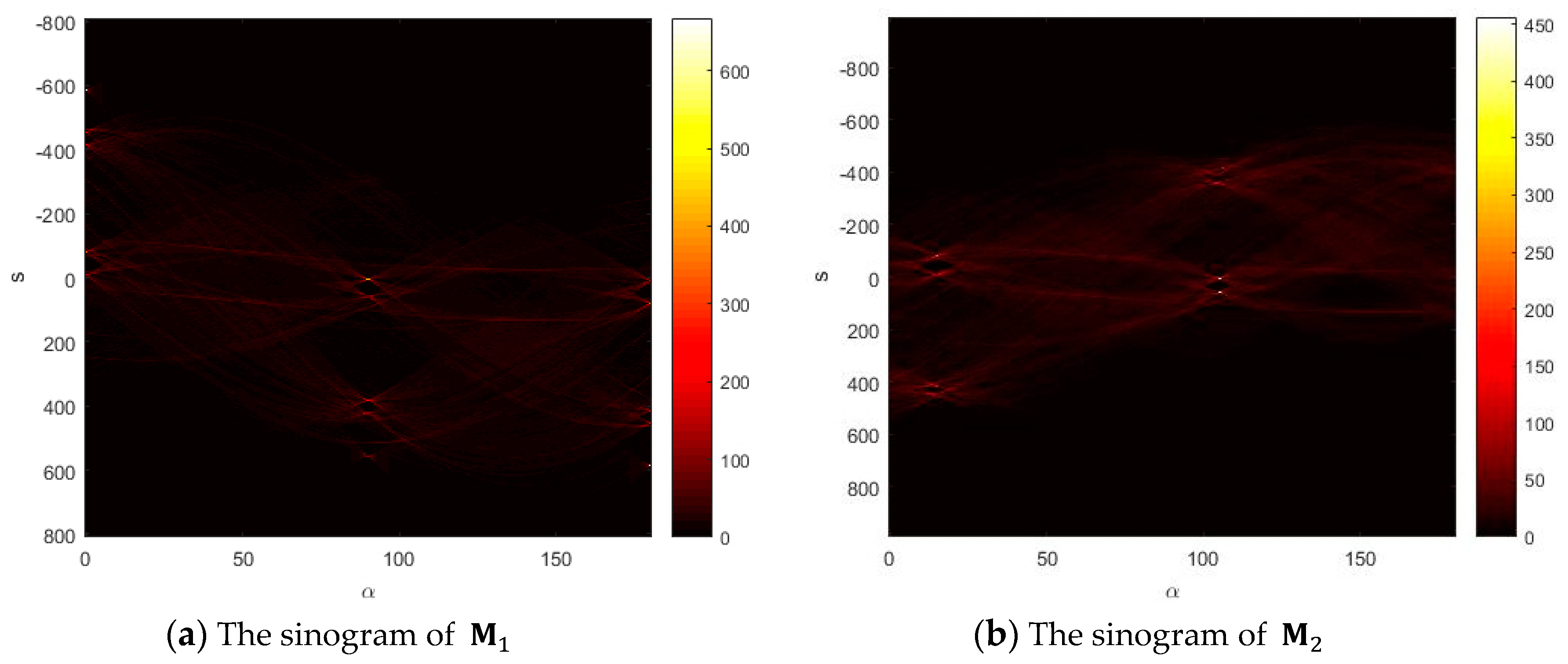
In the sinogram of a grid map, tomographic features are represented by the variation of column-wise levels according to α , which can give the clue to the shape of the grid map. Especially, α m a x at the location of the maximum level indicates that the most elongated direction of the grid map is α m a x 90 ° . For example, if the maximum intensity of S f in Figure 1b appears at ( 3 , 106 ° ) , the most elongated direction of f ( x , y ) is 16 ° . Therefore, the rotation angle between two grid maps can be estimated by comparing the locations indicating the maximum levels in their sinograms.
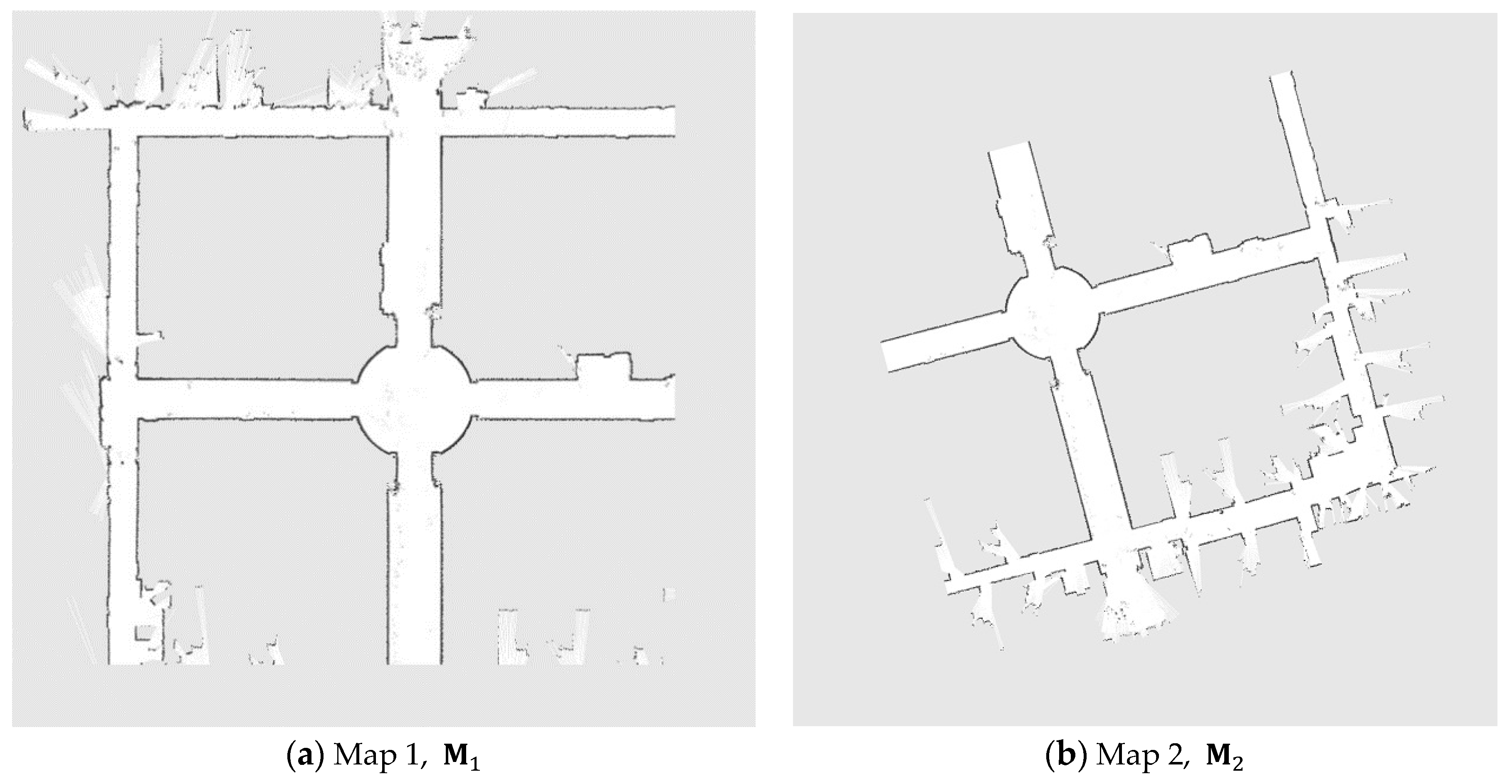
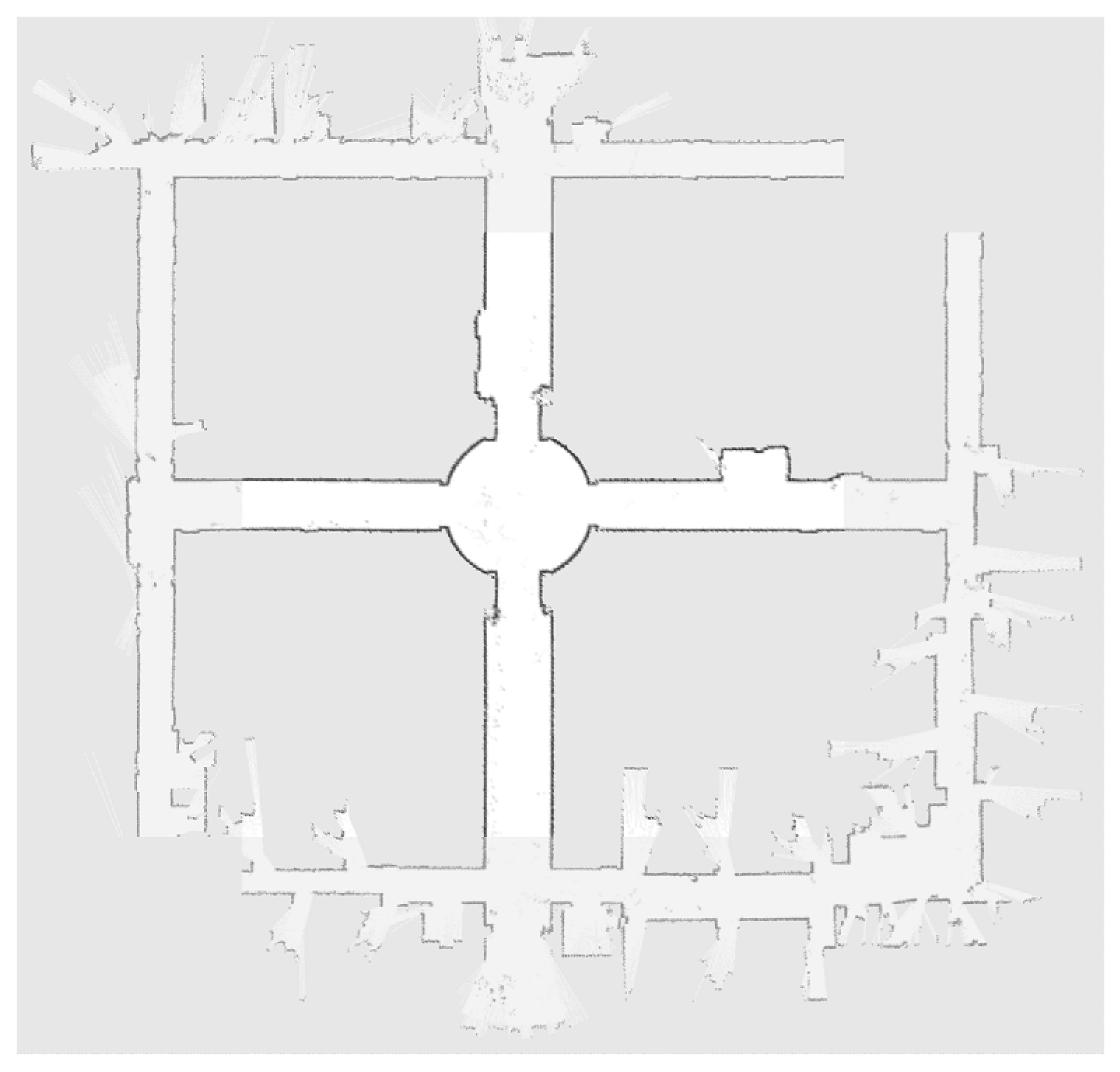
Figure 2 shows two individual grid maps, M 1 and M 2 , which are generated from the whole map of ACES3 [23]. The sizes of M 1 and M 2 are respectively r 1 × c 1 and r 2 × c 2 . Their sinograms are respectively generated for 0 ° α 180 ° as follows:
S M 1 = R T M 1 ( s , α ) ,                                 ρ 1 s ρ 1 ,
S M 2 = R T M 2 ( s , α ) ,                                 ρ 2 s ρ 2 ,
where ρ n is the maximum s -value of S M n which are computed as follows:
ρ n = ( r n r n ) 2 + ( c n c n ) 2 + 1 ,
where the center of M 1 is ( r 1 , c 1 ) = ( r 1 + 1 2 , c 1 + 1 2 ) , and the center of M 2 is ( r 2 , c 2 ) = ( r 2 + 1 2 , c 2 + 1 2 ) . Here, denotes a ceiling function, and denotes a floor function.
Let ( s 1 , m a x , α 1 , m a x ) and ( s 2 , m a x , α 2 , m a x ) be the locations of the maximum levels in S M 1 and S M 2 . Then, the rotation angle Δ θ between M 1 and M 2 can be estimated as follows:
Δ θ = α 2 , m a x α 1 , m a x .
For example, the given maps and their sinograms as shown in Figure 3, since α 2 , m a x = 106 ° and α 1 , m a x = 91 ° , the rotation angle Δ θ = 15 ° . Note that in this work since the sinograms were extracted for the range of 0 α 180 ° as shown in Figure 3, the problem of Moebius strip symmetry of sinogram can be avoided. Consequently, the rotation angle is acquired from 180 ° Δ θ 180 ° .

3.1.2. Estimation of X - Y Translations

The tomographic features represented in sinograms also provide the clue to translations between two grid maps. Based on the estimated rotation angle Δ θ at the previous step, M ˜ 2 is obtained by rotating M 2 of Δ θ as follows:
M ˜ 2 a = T ( 0 , 0 , Δ θ ) M 2 a ,
where M ˜ 2 a and M 2 a are the alternative forms of M ˜ 2 and M 2 , respectively. The alternative form is another version of the original grid map, which is a 3 × N o c c matrix for the convenient matrix calculation, where N o c c is the number of occupied grid points. The first and second rows represent the x and y coordinates of occupied grid points, respectively. The last row is filled with 1 for the convenient matrix multiplication.
The size of M ˜ 2 is r ˜ 2 × c ˜ 2 . For 0 ° α 180 ° , the sinogram of M ˜ 2 is generated as follows:
S M ˜ 2 = R T M ˜ 2 ( s , α ) ,                                 ρ ˜ 2 s ρ ˜ 2 ,
where ρ ˜ 2 is the maximum s -value of S M ˜ 2 , which is computed as follows:
ρ ˜ 2 = ( r ˜ 2 r ˜ 2 ) 2 + ( c ˜ 2 c ˜ 2 ) 2 + 1 ,
The estimation of each translation can be obtained by finding the s -value which maximizes the cross-correlation between two p a r t i a l   s i n o g r a m s corresponding to a certain α -value. Each partial sinogram indicates the distribution of grids along the α direction, which means that it is the distribution of s corresponding to the α -value. Given S M n with 2 ρ n + 1 rows and ϕ n columns generated from the n -th map M n with r n rows and c n columns, the partial sinogram corresponding to the α -value is defined as follows:
P S M n α ( t ) = S M n ( t ρ n 1 , α ) ,         0 < t 2 ρ n + 1 ,
where ρ n is the maximum s -value of S M n , which can be computed by (6).
Especially, the partial sinogram of s for x and y axes may be simply computed with α = 180 ° and α = 90 ° such as P S M n 180 ° ( s ) and P S M n 90 ° ( s ) . However, since the sizes of the maps are generally different as shown in M 2 and M ˜ 2 , the partial sinograms for x and y axes are redefined to obtain the cross correlation function between them. In other words, they should be represented with the same dimension, which is defined as the maximum size of the maps M 1 and M ˜ 2 as follows: r m = max ( r 1 , r ˜ 2 ) and c m = max ( c 1 , c ˜ 2 ) . Then, the partial sinograms of M 1 for x and y axes are respectively redefined by
P S M 1 X ( i ) = ( P S M 1 180 ° ( i + ρ 1 c m ) 1 i 2 c m + 1 0 otherwise ,
P S M 1 Y ( j ) = ( P S M 1 90 ° ( j + ρ 1 r m ) 1 j 2 r m + 1 0 otherwise ,
where ρ 1 = 2 ρ 1 + 1 2 , c m = 2 c m + 1 2 , and r m = 2 r m + 1 2 .
The partial sinograms of M ˜ 2 for x and y axes are similarly redefined. Then, the X and Y translation amounts between M 1 and M ˜ 2 can be estimated by finding the arguments which maximize the discrete cross correlation between their partial sinograms. The discrete cross correlation between them for x -axis is computed as follows:
C C X M 1 M ˜ 2 ( τ ) = ( k = X S M 1 ( K + τ ) X S M ˜ 2 ( k ) 1 τ c m 0 otherwise ,
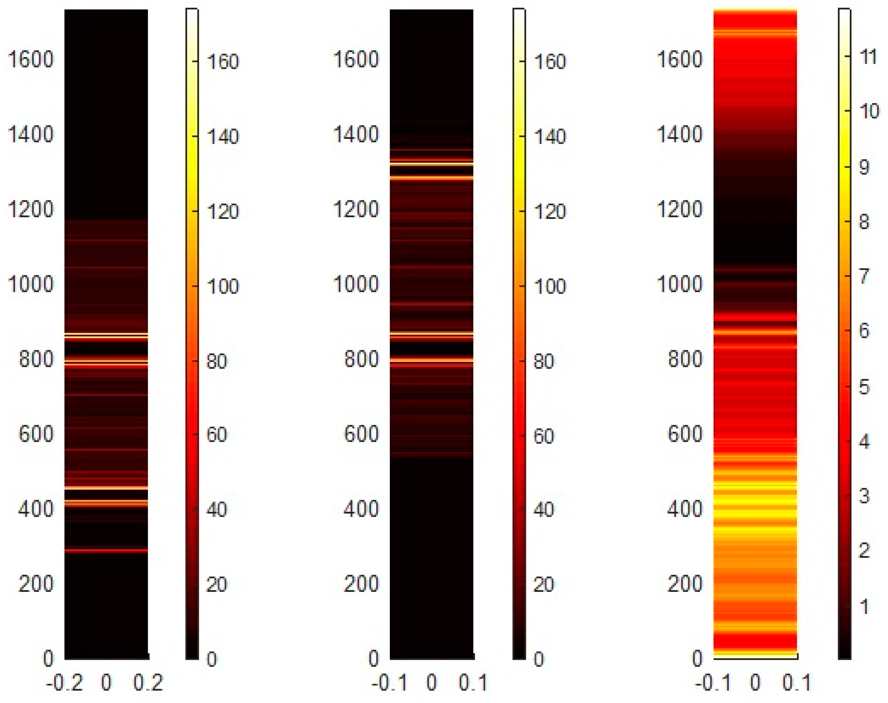
where c m is the maximum column size of the map matrices M 1 and M ˜ 2 . Within the maximum range, the discrete cross-correlation is computed. Otherwise, it is zero. Figure 4 shows the visualization of P S M 1 X , P S M ˜ 2 X , and C C X M 1 M ˜ 2 , respectively. Similarly, the cross correlation between them for y -axis is computed as follows:
C C Y M 1 M ˜ 2 ( υ ) = ( l = Y S M 1 ( l + υ ) Y S M ˜ 2 ( l ) 1 υ r m 0 otherwise ,
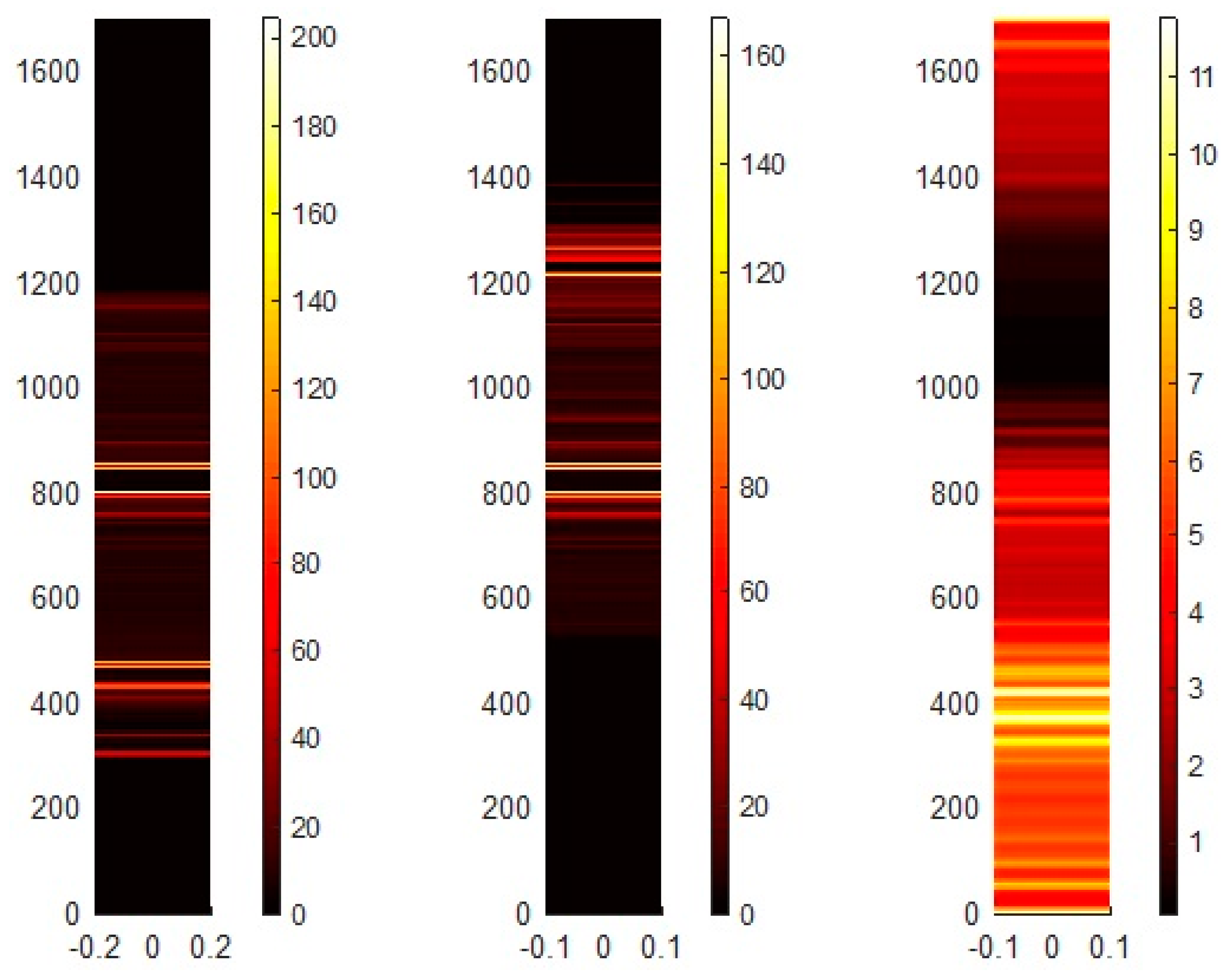
where r m is the maximum row size of the map matrices M 1 and M ˜ 2 . Within the maximum range, the discrete cross-correlation is computed. Otherwise, it is zero. Figure 5 shows the visualization of P S M 1 Y , P S M ˜ 2 Y , and C C Y M 1 M ˜ 2 , respectively.
Finally, the X -translation and the Y -translation amounts between the maps are respectively obtained by selecting the argument which maximizes C C X M 1 M ˜ 2 and C C Y M 1 M ˜ 2 as follows:
Δ x = argmax τ   C C X M 1 M ˜ 2 ( τ ) ,
Δ y = argmax υ   C C Y M 1 M ˜ 2 ( υ ) .
Then, since the elements of the MTM between M 1 and M 2 are completely computed, M 2 can be merged into M 1 by rotation and translations.

3.2. Search Space Determination with Gaussian Mixture Models

The MTM estimated by matching the tomographic features of the individual maps may be inaccurate due to inevitable transformation errors and local maxima. The more accurate MTM can be obtained by optimization algorithms, but it requires too much computation time because the initially given search space is too large. In the proposed method, the search space can be efficiently determined using Gaussian mixture models (GMMs). The search range for the rotation angle is determined using a univariate Gaussian mixture model (UGMM), and the search space for the translations is determined using a multivariate Gaussian mixture model (MGMM).
First, the numbers of the reference points in S M 1 and S M 2 to determine the means and standard deviations of the univariate random variable for the rotation angle are respectively determined with the concept of entropy as follows:
N θ 1 = p 1 log 2 p 1 ,
N θ 2 = p 2 log 2 p 2 ,
where p 1 and p 2 are respectively the histograms of S M 1 and S M 2 . Then, the reference points for each sinogram are extracted by N θ 1 and N θ 2 in the descending order of the intensities of S M 1 and S M 2 as follows: Θ 1 = { α 1 , n } n = 1 , , N U G M M and Θ 2 = { α 2 , n } n = 1 , , N U G M M where N U G M M = min ( N θ 1 , N θ 2 ) , which is the number of the univariate random variables for the rotation angle. Then, means of the univariate random variable for the rotation angle are calculated as follows:
Ω θ = { α 2 , n α 1 , n     |     α 1 , n Θ 1 , α 2 , n Θ 2 } .
The above equation can be rewritten for the simplicity as follows: Ω θ = { β i | β i Ω θ } i = 1 , , N U G M M . The standard deviations of the univariate random variable is calculated as follows:
Σ θ = { σ θ , i | σ θ , i = ( p 1 log 2 p 1 ) ( p 2 log 2 p 2 ) } i = 1 , , N U G M M
Next, the means of the multivariate random variable for X and Y translations are respectively calculated using the sets of peak locations, Λ X and Λ Y which are sorted in the descending order of the correlation values of C C X M 1 M ˜ 2 and C C Y M 1 M ˜ 2 as follows:
Ω X = { τ n     |     τ n Λ X } n = 1 , , N M G M M ,
Ω Y = { ν m     |     ν m Λ Y } m = 1 , , N M G M M ,
where N M G M M = max ( p x log 2 p x , p y log 2 p y ) . Here, p x and p y are the histograms of C C X M 1 M ˜ 2 and C C Y M 1 M ˜ 2 , respectively. The standard deviations for the multivariate random variables are respectively calculated using the obtained observation points and the coarse MTM as follows:
Σ X = { σ x , i | σ x , i = ( p x log 2 p x ) ( p y log 2 p y ) } i = 1 , , N M G M M ,
Σ Y = { σ y , i | σ y , i = ( p x log 2 p x ) ( p y log 2 p y ) } i = 1 , , N M G M M .
Now, if there is no dependency among the variances, the covariance matrices of the multivariate random variables for X and Y translations are calculated using Σ X and Σ Y as follows:
Σ X Y = { [ σ x , i 0 0 σ y , i ] |     σ x , i Σ X ,     σ y , i Σ Y } i = 1 , , N M G M M

3.3. Optimization for the More Accurate MTM

The estimation results of the MTM with tomographic features presented in Section 3.1 may contain slight mismatches due to inevitable sensing errors. If the multi-robot system requires a more accurate MTM, the accuracy of the MTM can be improved by modeling the objective function and optimizing it. In this paper, we propose a new objective function based on tomographic information. Also, this paper presents how the Monte-Carlo optimization (MCO) algorithm can be applied to map merging with the proposed objective function. The overall optimization algorithm is summarized in Table 1.
The sampling process in the MCO is divided into two categories such as the rotation angle sampling from the UGMM and the translation amounts sampling from the MGMM. One-dimensional candidates for the rotation angle and two-dimensional candidates for the translation amounts are respectively sampled from the UGMM and the MGMM as follows:
T ^ θ N 1 ( Ω θ , Σ θ ) ,
T ^ x y N 2 ( [ Ω X Ω Y ] , [ Σ X 0 0 Σ Y ] ) ,
where the numbers of components in T ^ θ and T ^ x y are respectively represented as N s , θ and N s , x y , which are user-defined parameters. Then, the set of three-dimensional combined candidates, Γ = { T ^ 1 , , T ^ N s } , are obtained by connecting each candidate in T ^ θ with each candidate in T ^ x y , where N s = N s , θ N s , x y .
The sampled configuration is evaluated by the objective function which indicates how the tomographically salient features in the individual maps are matched as follows:
Υ n ( M 1 , T ^ n M 2 ) = k = 1 K d [ P S ^ M 1 α ( k ) P S ^ T ^ n M 2 α ( k ) ] ,
where K d is the length of saliency check points. P S ^ M 1 α and P S ^ T ^ n M 2 α are respectively sorted forms in the descending order of P S M 1 α and P S T ^ n M 2 α , where α is generally set to 90 ° or 180 ° . After the evaluation of all sampled configurations is over, the best MTM for map merging is obtained by:
T b e s t = argmax T ^ n Γ   Υ n ( M 1 , T ^ n M 2 ) .

4. Evaluation Results

4.1. Simulation Results

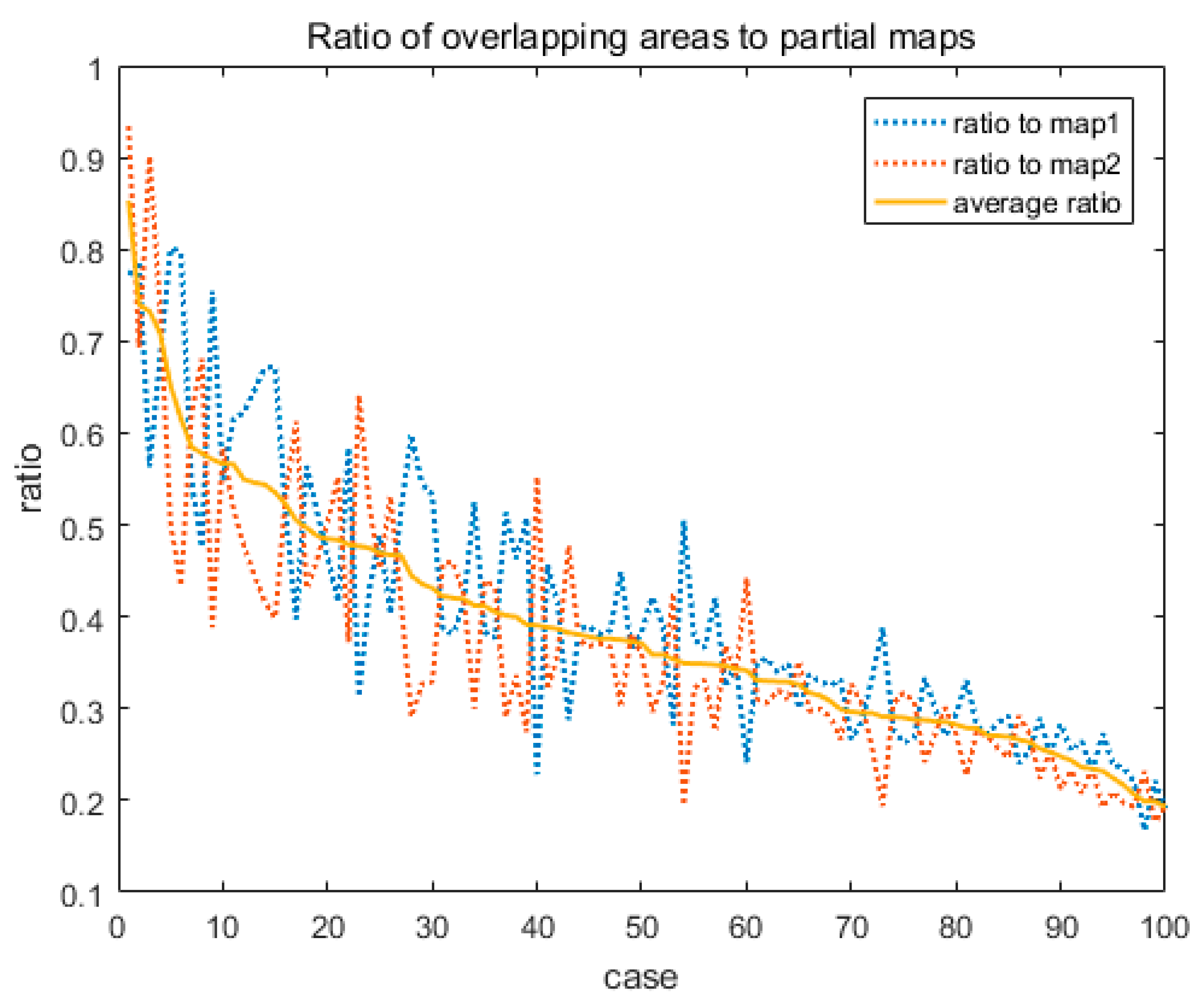
To test and evaluate the performance of the proposed method, the individual maps were generated from the whole map produced by one of the public datasets [23], which is also used to describe the proposed method in the previous sections. The result of merging the individual maps using the proposed method is shown in Figure 6. The proposed method does not always outperform the other map merging methods. This is because the accuracy of indirect map merging without any initial correspondences methods depends on not only the size of overlapping areas but also the shape of overlapping areas. A map merging method works well in a certain case with overlapping areas, but it does not work well in other cases with the same amount of overlapping areas because its shape is hard for the method. In other words, even though there are enough overlapping areas, the method may not work well due to the shape of the overlapping areas. Therefore, the accuracy of map merging methods should be evaluated by average and standard deviation from the various cases of overlapping areas as many as possible. Therefore, for the quantitative evaluation of the proposed map merging method, one hundred different pairs of individual maps were randomly produced from the whole map and rearranged according to the average ratio of overlapping areas to individual maps as shown in Figure 7. The maximum average ratio and the minimum average ratio were 0.8532 and 0.1929, respectively. To evaluate the accuracy of a result MTM, T r e s u l t , obtained by the proposed method or other methods, a matching index Ψ was defined as follows:
Ψ ( M 1 , T r e s u l t M 2 ) = x = a 1 a 2 y = b 1 b 2 M 1 ( x , y ) [ T r e s u l t M 2 ( x , y ) ] N o v e r l a p
where N o v e r l a p is the number of occupied grids in overlapping areas, and the sizes of M 1 and M 2 are commonly as a 1 x a 2 and b 1 y b 2 .
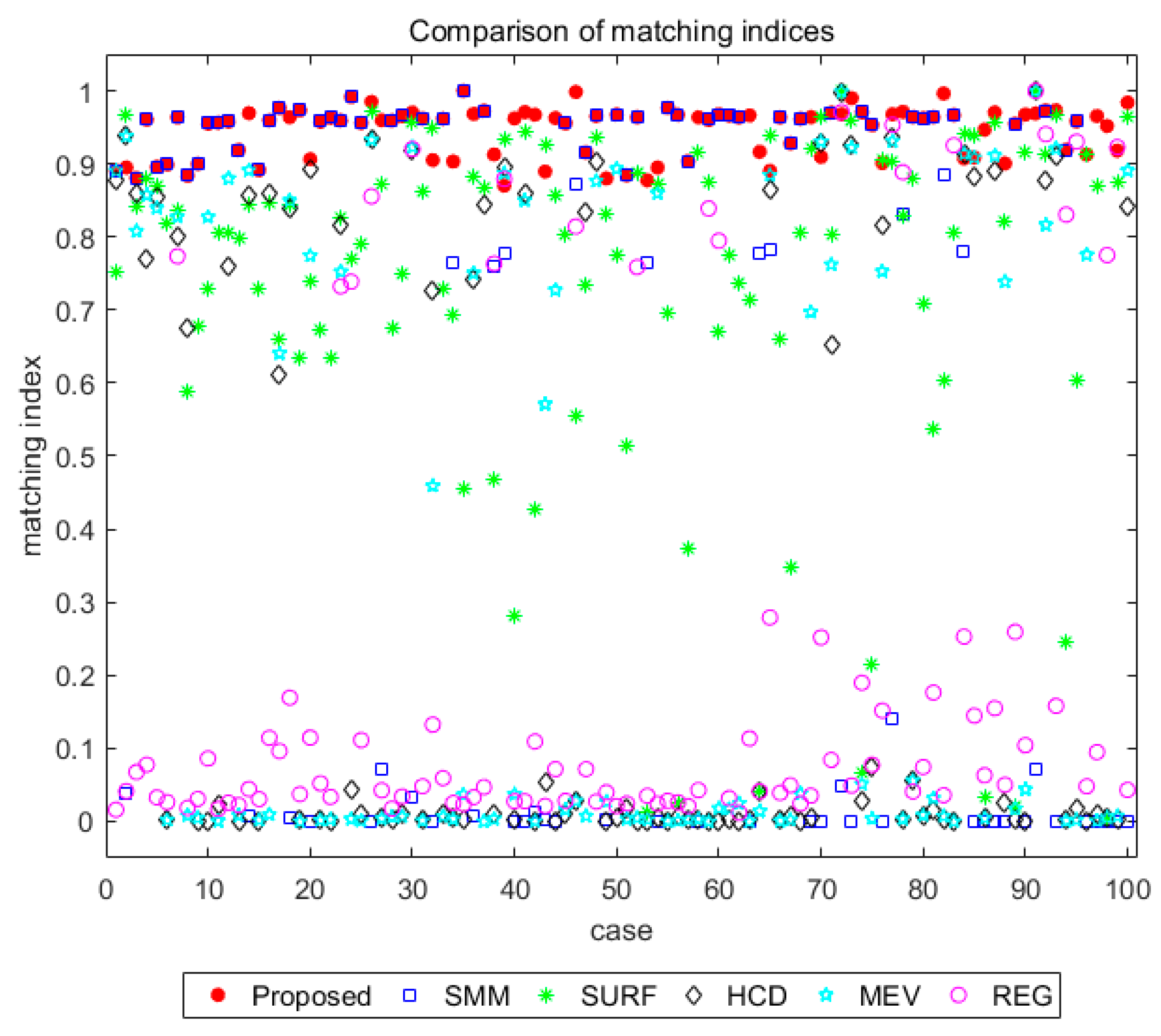
The performance of the proposed method was compared with spectra-based map merging (SMM) [18] because it is a well-known grid map merging method with unknown initial correspondences. Also, the proposed method was compared with a local feature descriptor matching method such as SURF (speeded up robust features) [24], Harris corner detection (HCD) [25], and maximum eigenvalue-based corner detection (MEV) [26]. Also, the proposed method was compared with the intensity-based image registration method (REG) because it is similar to this work in the context that each individual map can be regarded as a binary image. The comparison results with the different pairs of individual maps are shown in Figure 8. In some cases, the accuracy of the proposed method was similar to others or lower than others, but the differences were not significant. The proposed method showed consistently good accuracy and averagely better performance than others. For the statistical comparison and analysis, the averages and standard deviations of the matching indices with the proposed method and other methods are summarized in Table 2, which indicates that the proposed method can work consistently better than the other methods.

4.2. Experimental Results

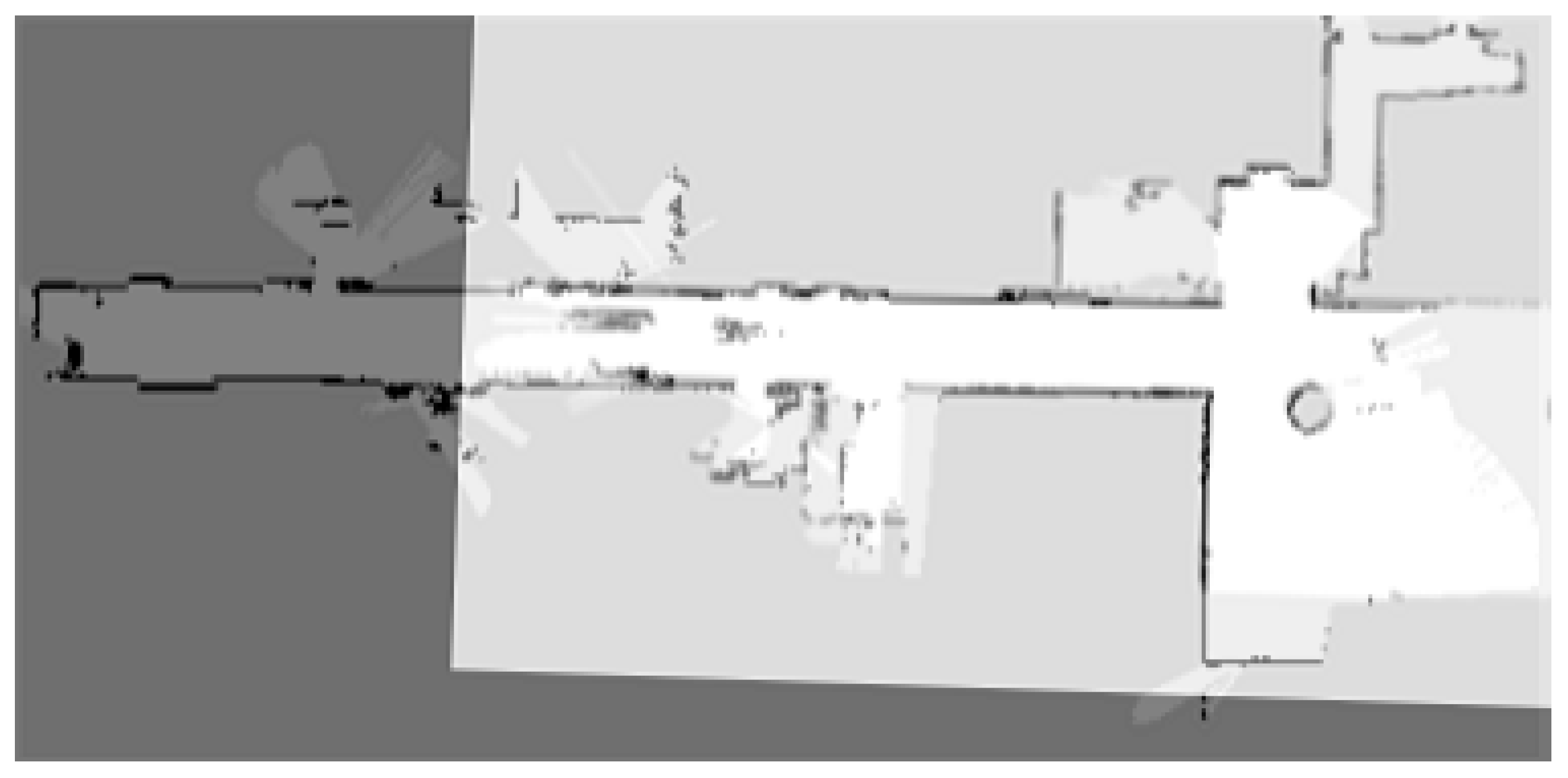
The performance of the proposed method was also tested by individual maps produced by a real multi-robot system in indoor environments. The multi-robot system was composed of three mobile robots with laser scan sensors and a wireless router. The robot was Pioneer3-DX, and the laser scan sensor was Hokuyo UTM-30LX. The indoor environment was the third floor of the Automation and Systems Research Institute at Seoul National University. Its size is about 48 m × 17 m. Two individual maps were produced by the multiple robots using our multi-robot SLAM framework as shown in Figure 9, and the sinograms of them are shown in Figure 10. The individual maps were successfully merged by the proposed method as shown in Figure 11.
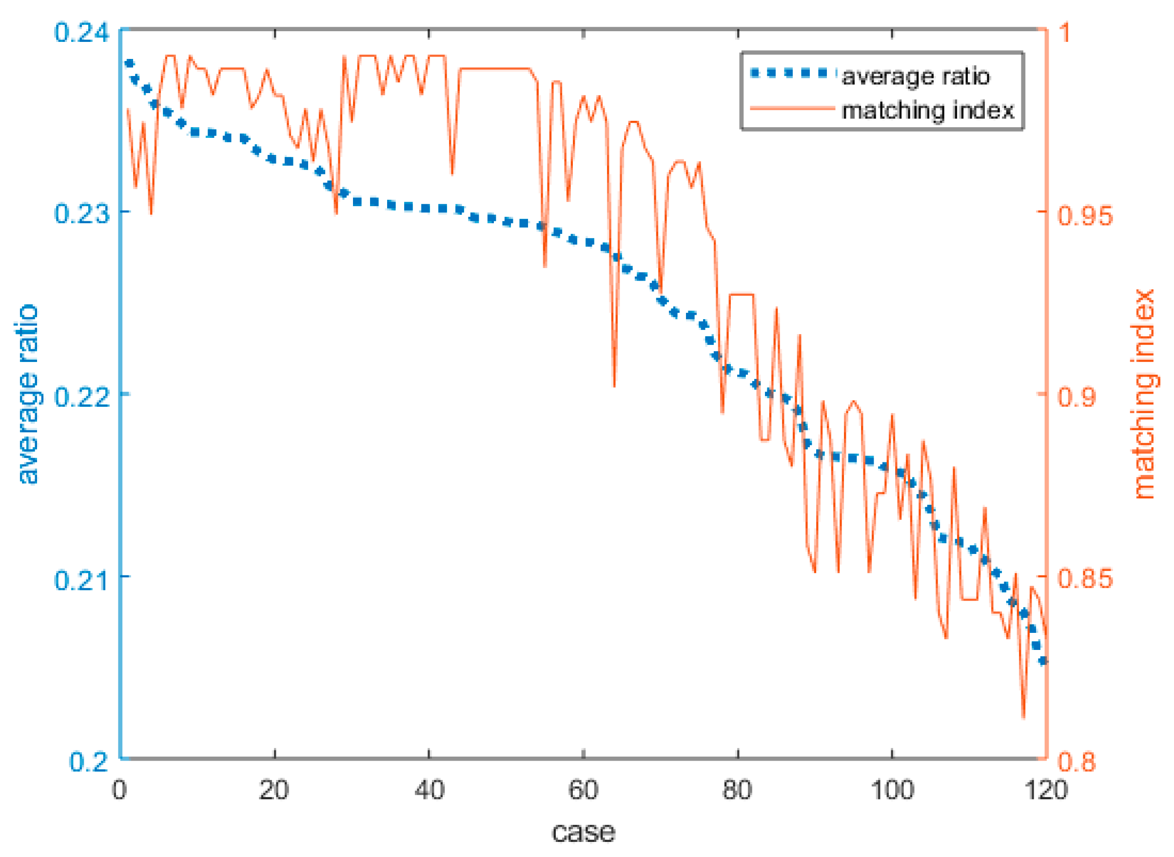
To evaluate the accuracy of the proposed algorithm according to the ratio of overlapping areas to individual maps, the matching indices should be measured with various cases in the experimental environment. Thus, the translation amounts and the rotation angles were randomly selected and combined into various pairs of individual maps. Then, they were rearranged according to the average ratio of overlapping areas to individual maps, which are represented by the blue dotted line as shown in Figure 12. Differently from the simulation results, the accuracy of map merging was significantly affected by the number of overlapping areas due to the errors in individual maps. Therefore, the matching indices were analyzed according to the average ratio of overlapping areas to individual maps, which are represented by the red solid line as shown in Figure 12. In the microscopic context, it was difficult to find any patterns for the matching index between the individual maps since there were many abrupt changing points in the matching index. But, in the macroscopic context, the matching index gradually decreases according to the average ratio. Even though the matching index decreased as the average ratio decreased, the proposed method showed relatively high matching indices for all the cases of individual maps.
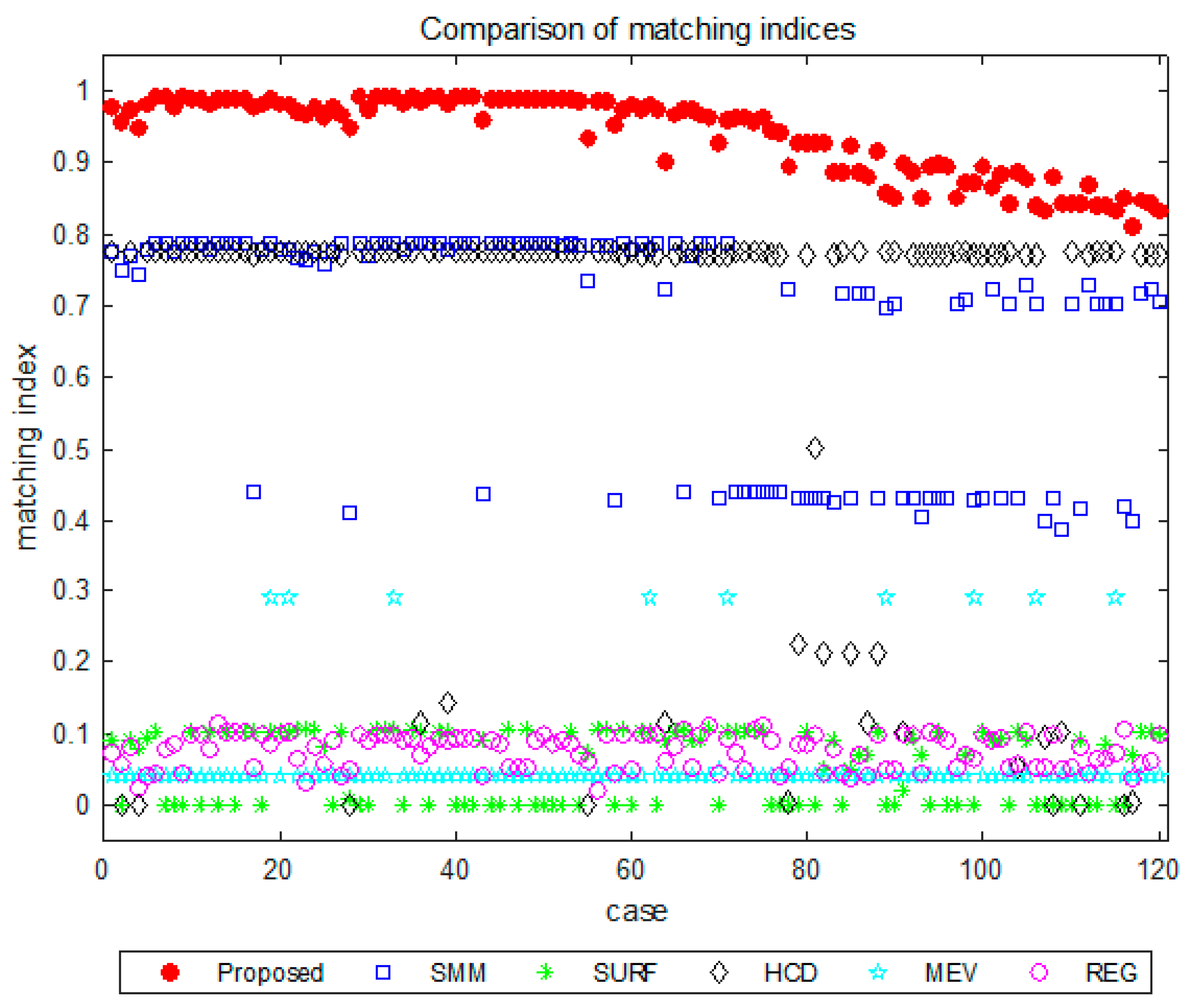
For more comparative analysis, the matching indices of the proposed method with the different pairs of individual maps were compared with those of the SMM, SURF, HCD, MEV, and REG, which are shown in Figure 13. For the statistical comparison and analysis, the averages and standard deviations of the matching indices with the proposed method and other methods are summarized in Table 2. The SMM showed relatively high matching indices, but its accuracy abruptly decreased for a low average ratio of overlapping areas. The HCD also showed relatively high matching indices, which was much different from the simulation results. However, its abrupt decrease in the accuracy of map merging was larger than the SMM, and its average matching index was also smaller than not only the proposed method but also the SMM. The SURF showed low matching indices even though it showed relatively high matching indices for map merging in simulations. The MEV and REG did not show acceptable performance. These varying results indicate that the accuracy of the descriptor-based map matching methods highly depends on the shape and quality of individual maps. In other words, although a descriptor-based map matching method was good for map merging in a certain environment, its accuracy could not be guaranteed for map merging in different environments. Consequently, the matching indices of the proposed method were higher than those of other methods, which verifies that the proposed method is more accurate than the others.
The computational times were quantitatively compared using averages and standard deviations from as shown in Table 3. Since the sizes of individual maps in simulations were larger than those in experiments, the computational times in simulations were overall smaller than those in experiments. The average of the computational times of the proposed method was larger than the others except for REG. This is because the Monte-Carlo optimization included in the proposed method to improve the accuracy of map merging requires much computational time due to its iterative property. Note that the computational times decreased by about 56.64% when Monte-Carlo optimization is excluded from the proposed method, which was similar to the others as shown in Table 3. If the total computational time of the proposed method is larger than the update period of the collective map of the multi-robot system, one can consider acceleration methods based on graphics processing unit (GPU) [27] or field-programmable gate array (FPGA) [20], which will be researched more thoroughly in my future work.

5. Conclusions

The grid map merging without any information on initial robot poses or inter-robot measurements is one of the challenging problems in multi-robot systems. Especially, if the overlapping area between maps is insufficient, it is too difficult to accurately merge the given individual maps. This paper proposed a new map merging method using tomographic features, which can be conducted well with relatively small overlapping area. The evaluation results showed that the proposed method can successfully merge the given individual maps with relatively small overlapping areas, and its accuracy was higher than other map merging methods.

Acknowledgments

This work was supported by the National Research Foundation of Korea(NRF) grant funded by the Korea government(MSIT) (No. 2019R1G1A1100597).

Conflicts of Interest

The author declares no conflict of interest.

References

  1. Lee, H.C.; Lee, B.H. Enhanced-spectrum-based map merging for multi-robot systems. Adv. Robot. 2013, 2, 1285–1300. [Google Scholar] [CrossRef]
  2. Konolige, K.; Fox, D.; Limketkai, B.; Ko, J.; Stewart, B. Map merging for distributed robot navigation. In Proceedings of the IEEE/RSJ International Conference on Intelligent Robots and Systems, Las Vegas, NV, USA, 27–31 October 2003. [Google Scholar]
  3. Zhou, X.S.; Roumeliotis, S.I. Robot-to-robot relative pose estimation from range measurements. IEEE Trans. Robot. 2008, 24, 1379–1393. [Google Scholar] [CrossRef] [Green Version]
  4. Tungadi, F.; Lui, W.L.D.; Kleeman, L.; Jarvis, R. Robust online map merging system using laser scan matching and omnidirectional vision. In Proceedings of the IEEE/RSJ International Conference on Intelligent Robots and Systems, Taipei, Taiwan, 18–22 October 2010. [Google Scholar]
  5. Kim, B.; Kaess, M.; Fletcher, L.; Leonard, J.; Bachrach, A.; Roy, N.; Teller, S. Multiple relative pose graphs for robust cooperative mapping. In Proceedings of the IEEE International Conference on Robotics and Automation, Anchorage, AK, USA, 3–8 May 2010. [Google Scholar]
  6. Li, H.; Tsukada, M.; Nashashibi, F.; Parent, M. Multivehicle cooperative local mapping: A methodology based on occupancy grid map merging. IEEE Trans. Intell. Transp. Syst. 2014, 15, 2089–2100. [Google Scholar] [CrossRef] [Green Version]
  7. Dinnissen, P.; Givigi, S.N.; Schwartz, H.M. Map merging of multi-robot SLAM using reinforcement learning. In Proceedings of the IEEE International Conference on Systems, Man, and Cybernetics, Seoul, Korea, 14–17 October 2012. [Google Scholar]
  8. Garcia-Cruz, X.M.; Sergiyenko, O.Y.; Tyrsa, V.; Rivas-Lopez, M.; Hernandez-Balbuena, D.; Rodriguez-Quiñonez, J.C.; Basaca-Preciado, L.C.; Mercorelli, P. Optimization of 3D laser scanning speed by use of combined variable step. Opt. Lasers Eng. 2014, 54, 141–151. [Google Scholar] [CrossRef]
  9. Lindner, L.; Sergiyenko, O.; Rivas-López, M.; Ivanov, M.; Rodríguez-Quiñonez, J.C.; Hernández-Balbuena, D.; Flores-Fuentes, W.; Tyrsa, V.; Muerrieta-Rico, F.N.; Mercorelli, P. Machine vision system errors for unmanned aerial vehicle navigation. In Proceedings of the IEEE International Symposium on Industrial Electronics, Edinburgh, UK, 19–21 June 2017; pp. 1615–1620. [Google Scholar]
  10. Lee, H.C.; Lee, S.H.; Choi, M.H.; Lee, B.H. Probabilistic map merging for multi-robot RBPF-SLAM with unknown initial poses. Robotica 2012, 30, 205–220. [Google Scholar] [CrossRef]
  11. Lee, H.C.; Cho, Y.J.; Lee, B.H. Accurate map merging with virtual emphasis for multi-robot systems. Electron. Lett. 2013, 49, 932–934. [Google Scholar] [CrossRef]
  12. Birk, A.; Carpin, S. Merging occupancy grid maps from multiple robots. Proc. IEEE 2006, 94, 1384–1397. [Google Scholar] [CrossRef]
  13. León, A.; Barea, R.; Bergasa, L.M.; López, E.; Ocaña, M.; Schleicher, D. SLAM and map merging. J. Phys. Agents 2009, 3, 13–23. [Google Scholar]
  14. Wang, K.; Jia, S.; Li, Y.; Li, X.; Guo, B. Research on map merging for multi-robotic system based on RTM. In Proceedings of the IEEE International Conference on Information and Automation, Shenyang, China, 6–8 June 2012. [Google Scholar]
  15. Saeedi, S.; Paull, L.; Trentini, M.; Li, H. Multiple robot simultaneous localization and mapping. In Proceedings of the IEEE/RSJ International Conference on Intelligent Robots and Systems, San Francisco, CA, USA, 25–30 September 2011. [Google Scholar]
  16. Saeedi, S.; Paull, L.; Trentini, M.; Li, H. A neural network-based multiple robot simultaneous localization and mapping. IEEE Trans. Neural Netw. 2011, 22, 2376–2387. [Google Scholar] [CrossRef] [PubMed]
  17. Howard, A. Multi-robot simultaneous localization and mapping using particle filters. Int. J. Robot. Res. 2006, 25, 1243–1256. [Google Scholar] [CrossRef] [Green Version]
  18. Carpin, S. Fast and accurate map merging for multi-robot systems. Auton. Robots 2008, 25, 305–316. [Google Scholar] [CrossRef]
  19. Lee, H.C.; Lee, B.H. Improved feature map merging using virtual supporting lines for multi-robot systems. Adv. Robot. 2012, 25, 1675–1696. [Google Scholar] [CrossRef]
  20. Lee, H.; Kim, K.; Kwon, Y.; Hong, E. Real-time particle swarm optimization on FPGA for the optimal message-chain structure. Electronics 2018, 7, 274. [Google Scholar] [CrossRef] [Green Version]
  21. Lee, H.; Kim, K.; Kwon, Y. Efficient and reliable bus controller operation with particle swarm optimization in MIL-STD-1553B. In Proceedings of the Asia-Pacific International Symposium on Aerospace Technology, Seoul, Korea, 16–18 October 2017. [Google Scholar]
  22. Resnick, J. The radon transforms and some of its applications. IEEE Trans. Acoust. Speech Signal Process. 1985, 33, 338–339. [Google Scholar] [CrossRef]
  23. Stachniss, C. Robotics 2D-Laser Datasets. Available online: http://www.ipb.uni-bonn.de/datasets (accessed on 12 December 2019).
  24. Bay, H.; Tuytelaars, T.; Gool, L.V. SURF: Speeded up robust features. In Proceedings of the European Conference on Computer Vision, Graz, Austria, 7–13 May 2006. [Google Scholar]
  25. Harris, C.; Stephens, M. A combined corner and edge detector. In Proceedings of the Alvey Vision Conference, Roke Manor, UK, 1 January 1988. [Google Scholar]
  26. Shi, J.; Tomasi, C. Good features to track. In Proceedings of the IEEE Conference on Computer Vision and Pattern Recognition, Seattle, WA, USA, 21–23 June 1994. [Google Scholar]
  27. Zhang, C.; Weingartner, S.; Moeller, S.; Uğurbil, K.; Akçakaya, M. Fast GPU Implementation of a scan-specific deep learning reconstruction for accelerated magnetic resonance imaging. In Proceedings of the IEEE International Conference on Electro/Information Technology, Rochester, MI, USA, 3–5 May 2018; pp. 399–403. [Google Scholar]
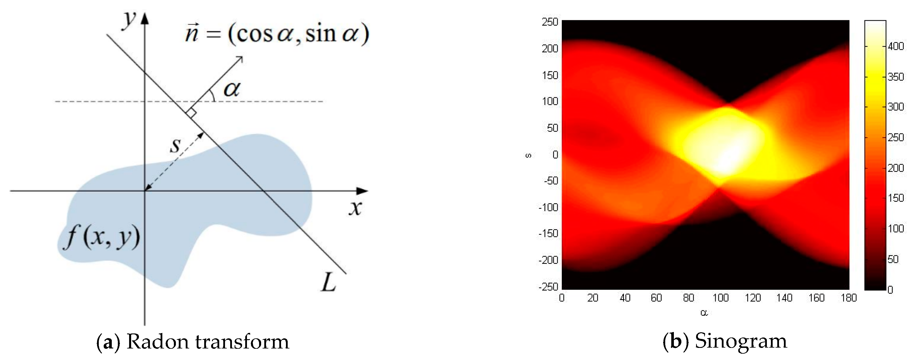
Figure 1. The concept of the Radon transform and sinogram. (a) A function f ( x , y ) on the 2D Euclidean space R 2 is transformed into a function on a new 2D space with α and s which defines the straight line L in R 2 . (b) The result of applying the Radon transform to f ( x , y ) is called s i n o g r a m .
Electronics 09 00107 g001
Figure 2. Two individual grid maps (a) M 1 and (b) M 2 . The black grids, the white grids, and the gray grids represent occupied, unoccupied, and unknown area, respectively. The map transformation matrix between them can be obtained by finding and aligning the overlapped areas between them.
Electronics 09 00107 g002
Figure 3. The sinograms of M 1 and M 2 . (a) The maximum intensity of the sinogram of M 1 appears at ( 136 , 91 ° ) . (b) The maximum intensity of the sinogram of M 2 appears at ( 997 , 106 ° ) .
Electronics 09 00107 g003
Figure 4. The partial sinograms of M 1 and M ˜ 2 for x -axis (left and middle) and their normalized cross-correlation (right). The X -translation amount is estimated by matching the partial sinograms where α = 180 ° .
Electronics 09 00107 g004
Figure 5. The partial sinograms of M 1 and M ˜ 2 for y -axis (left and middle) and their normalized cross-correlation (right). The Y -translation amount is estimated by matching the partial sinograms where α = 90 ° .
Electronics 09 00107 g005
Figure 6. The result of merging M 1 and M 2 . The overlapping areas are represented by white grids.
Electronics 09 00107 g006
Figure 7. The ratio of overlapping areas to the various pairs of the individual maps. One hundred different pairs of individual maps were randomly produced from the whole map in simulations and rearranged according to the average ratio of overlapping areas to individual maps.
Electronics 09 00107 g007
Figure 8. Comparison of matching indices with the proposed method and other methods according to the different pairs of individual maps produced from the whole map in simulations. The matching indices with the proposed method were consistently higher than those with other methods.
Electronics 09 00107 g008
Figure 9. The individual maps, (a) M 3 and (b) M 4 , produced by three robots in indoor environments.
Electronics 09 00107 g009
Figure 10. The sinograms, S M 3 and S M 4 , of the individual maps produced by three robots in indoor environments.
Electronics 09 00107 g010
Figure 11. The result of merging the individual maps, M 3 and M 4 , which are produced from experiments.
Electronics 09 00107 g011
Figure 12. The average ratio of overlapping areas to the various pairs of the individual maps of the merged map in experiments and the corresponding matching indices. One-hundred and twenty different pairs of individual maps were randomly produced from the merged map and rearranged according to the average ratio of overlapping areas to individual maps. The matching index between the individual maps decreases macroscopically according to the average ratio.
Electronics 09 00107 g012
Figure 13. Comparison of matching indices with the proposed method and other methods according to the different pairs of individual maps produced from real experimental data. The matching indices with the proposed method were consistently higher than those with other methods.
Electronics 09 00107 g013
Table 1. Optimization to acquire the more accurate MTM (map transformation matrix).
Algorithm:Monte-Carlo optimization for the more accurate MTM
Input:Given individual maps: M 1 and M 2
The mean set and variance set of the UGMM: Ω θ and Σ θ
The mean vector set and covariance set of the MGMM: Ω X , Ω Y , and Σ X Y
Output:The best MTM in T b e s t
1:Determine the number of samples N s , θ and N s , x y , where N s = N s , θ N s , x y
2:Initialize the objective function Υ
3:Sample one-dimensional candidates T ^ θ for the rotation angle in Eq. (27)
4:Sample two-dimensional candidates T ^ x y for the translation amounts in Eq. (28)
5:Obtain the set of three-dimensional combined candidates, Γ by combining T ^ θ and T ^ x y
6:Define the normal distribution with μ M N D and Σ M N D
7:for n = 1 to N S do
8:  Pick the n -the candiate T ^ n from Γ
9:  Obtain T ^ n M 2 by transforming M 2 using T ^ n
10:  Calculate the n -th value of the objective function Υ n ( M 1 , T ^ n M 2 , ) in Eq. (29)
11:end for
12:Take T n ^ indicating the maximum of the objective function in Eq. (30)
13:return T b e s t
Table 2. Comparison of the averages and standard deviations of matching indices with different methods in simulations and experimental data.
TypeProposed.SMMSURFHCDMEVREG
Sim.Avg.0.94570.59700.72440.32090.34870.2351
Std. Dev.0.03340.44420.25530.41220.41400.3292
Exp.Avg.0.93930.66650.05430.65070.05960.0756
Std. Dev.0.05520.15570.04830.26680.06580.0232
Table 3. Comparison of the averages and standard deviations of the computational times with different methods in simulations and experimental data (unit: sec).
TypeProposed.Proposed. w/o MCOSMMSURFHCDMEVREG
Sim.Avg.7.62193.30473.15275.37564.74754.887017.3969
Std. Dev.1.12820.30130.42350.39480.44630.39951.2543
Exp.Avg.0.37660.17810.15310.21980.42970.30170.6509
Std. Dev.0.04320.02230.12630.04800.09070.06130.1208