An Image Recognition-Based Approach to Actin Cytoskeleton Quantification

Abstract

Quantification of the actin cytoskeleton is of prime importance to unveil the cellular force sensing and transduction mechanism. Although fluorescence imaging provides a convenient tool for observing the morphology of the actin cytoskeleton, due to the lack of approaches to accurate actin cytoskeleton quantification, the dynamics of mechanotransduction is still poorly understood. Currently, the existing image-based actin cytoskeleton analysis tools are either incapable of quantifying both the orientation and the quantity of the actin cytoskeleton simultaneously or the quantified results are subject to analysis artifacts. In this study, we propose an image recognition-based actin cytoskeleton quantification (IRAQ) approach, which quantifies both the actin cytoskeleton orientation and quantity by using edge, line, and brightness detection algorithms. The actin cytoskeleton is quantified through three parameters: the partial actin-cytoskeletal deviation (PAD), the total actin-cytoskeletal deviation (TAD), and the average actin-cytoskeletal intensity (AAI). First, Canny and Sobel edge detectors are applied to skeletonize the actin cytoskeleton images, then PAD and TAD are quantified using the line directions detected by Hough transform, and AAI is calculated through the summational brightness over the detected cell area. To verify the quantification accuracy, the proposed IRAQ was applied to six artificially-generated actin cytoskeleton mesh work models. The average error for both the quantified PAD and TAD was less than 1.22${}^{\circ }$. Then, IRAQ was implemented to quantify the actin cytoskeleton of NIH/3T3 cells treated with an F-actin inhibitor (latrunculin B). The quantification results suggest that the local and total actin-cytoskeletal organization became more disordered with the increase of latrunculin B dosage, and the quantity of the actin cytoskeleton showed a monotonically decreasing relation with latrunculin B dosage.

1. Introduction

Currently, attention toward the cellular cytoskeleton is growing due to its significant abilities of affecting and reflecting the numerous physiological properties and states of the cell, such as the cell biomechanical properties [1,2,3], proliferation and migration [4,5], and the cell morphology [2,6,7]. As one of the three main components of the cellular cytoskeleton, the actin cytoskeleton (i.e., actin filaments) controls cell mechanotransduction dynamics through directly affecting the motility, contractility, and mechanical stability of the cells [2,6,8]. Specifically, the actin cytoskeleton responds to the external stimuli, such as the change of the substrate stiffness and external forces, applied on the cells through polymerization or depolymerization in order to regulate cellular physiological properties [9,10,11,12]. Therefore, the morphology of the actin cytoskeleton is of great importance in understanding the cellular dynamic mechanotransduction responses. Although studies have qualitatively shown the relative relation between the actin cytoskeleton morphology and the cell mechanical behavior [2,9], comprehensive approaches of accurately quantifying the general actin cytoskeleton morphology under usual handling conditions are still lacking. Therefore, to promote in-depth understanding of the cellular force transduction process, an actin cytoskeleton quantification framework must be developed first.

Morphology analysis of cells has been widely reported in the literature, among which shape analysis is the essential method to quantify the cellular morphology [13,14,15]. Shape analysis generally consists of three steps [16]: (1) segmenting the target region from the original image; (2) extracting the elements, such as the area, boundary, and skeleton from the target region; (3) quantifying and representing the needed shape features from extracted elements. The common shape features include the radius/diameter, area, moments, centroid, compactness, complexity, and convex hull [17,18,19]. However, such an approach cannot be directly applied to actin cytoskeleton analysis because the shape features developed do not match the random fiber mesh work topography of the actin cytoskeleton. Great efforts have been invested to generate more appropriate approaches for describing the organizational structure of the actin cytoskeleton. Nurit et al. (2003) proposed an algorithm called FiberScore to recognize and quantify various structural parameters, such as the total fiber-associated fluorescence, as well as the fiber length and orientation of the actin cytoskeleton, at a subcellular scale [2]. Alexander B et al. (2003) used an electron microscope and a light microscope to visualize the structural features of the actin mesh work in the advancing lamellipodia of living cells [20]. Takumi et al. (2010) quantified the cytoskeleton orientation, bundling, and density using the measurements of fluorescence microscopic images of plant cells with the stomatal movement [21]. Julian et al. (2012) developed an automatic method to reconstruct the orientation distribution of the actin cytoskeleton in the lamellipodium of migrating keratocytes using the topography data from the electron microscope [5]. Albertol et al. (2014) designed two computational tools to quantify actin stress fiber and the distribution of the actin cytoskeleton with respect to a normalized cellular morphology [1]. Basu et al. (2015) described a method for localizing and extracting filament distributions without any quantification of the actin filament state [22]. Mitchel et al. (2016) proposed a three-step extraction methodology for actin filaments’ extraction [4]. Kimori et al. (2016) used the mathematic morphology to quantify the shape features of the actin cytoskeleton in plant cells [13]. However, these methods either require specially-designed experiment hardware conditions [2,5,20], cannot quantify both the actin cytoskeleton quantity and alignment at the same time [1,4,22,23], or are primarily developed for plant cells in which the stomatal movementis set as the reference direction [13,21]; thus, they cannot be applied to quantify the actin cytoskeleton morphology of living animal cells under usual cell handling conditions. Therefore, this study aims to develop a new method to quantify the actin cytoskeleton morphology of living mammalian cells accurately, which can be easily implemented under standard cell handling conditions.

In this paper, we propose an image recognition-based actin cytoskeleton quantification (IRAQ) approach. IRAQ aims to quantify both the actin cytoskeleton orientation and quantity simultaneously through three morphology parameters: the partial actin-cytoskeletal deviation (PAD), the total actin-cytoskeletal deviation (TAD), and the average actin-cytoskeletal intensity (AAI), by processing fluorescence images of the actin cytoskeleton. PAD and TAD quantify the actin-cytoskeletal orientation distribution, which reflects the bundling and organization status, while AAI provides the average quantity of the actin cytoskeleton over the detected cell area. These three parameters can provide a quantitative insight into the actin cytoskeleton morphology, which have the abilities to reflect the cellular physiological properties. To process the actin cytoskeleton images, Canny and Sobel edge detectors [24] are applied to skeletonize the images for detecting the actin alignment deviation (PAD and TAD) and actin intensity (AAI), respectively. PAD and TAD are quantified using the direction of the lines detected by Hough transform, while AAI was calculated through the summational brightness and the cell area detected using the Sobel edge detection together with an image filling tool. For validation, IRAQ was used to quantify six artificially-generated actin cytoskeleton mesh work models. Furthermore, we applied IRAQ to study quantitatively the actin cytoskeleton change of NIH/3T3 cells caused by an F-actin inhibitor (latrunculin B).

2. Materials and Methods

2.1. Cell Preparation

2.1.1. Cell Culture

Primary mouse embryonic fibroblast cells (NIH/3T3) were maintained at $37{}^{\circ }$C in an incubator with a humidified atmosphere of $5\%$ CO${}_2$ in Dulbecco’s Modified Eagle’s Medium (ATCC, Rockville, MD, USA) and supplemented with 10% (v/v) calf bovine serum (Sigma-Aldrich, St. Louis, MO, USA) and 1% (v/v) penicillin-streptomycin (Gibco, Grand Island, NY, USA). Cells were seeded in a 35-mm tissue culture dish (Azzota Scientific, Claymont, DE, USA) and used 24 h after seeding.

2.1.2. Actin Cytoskeleton Treatment

To investigate the morphology of the actin cytoskeleton in different states, the cells were treated with latrunculin B (Millipore Sigma, Billerica, MA, USA) with the final concentrations of 0 nM (untreated or control condition), 187.5 nM, 375 nM, and 750 nM in the aforementioned cell culture medium and incubated for 30 min. The stock solution was made by dissolving latrunculin B in dimethyl sulfoxide (Sigma Aldrich, St. Louis, MO, USA).

2.1.3. Actin Cytoskeleton Staining

To observe the actin cytoskeleton, the cells were fixed for 10 min using $4\%$ paraformaldehyde (Alfa Aesar, Ward Hill, MA, USA) in PBS and permeabilized for 10 min using $0.1\%$ Triton-X (Fisher Scientific, Fair Lawn, NJ, USA) at room temperature. The actin cytoskeleton was then stained with Actin-stain${}^{\mathrm{TM}}$ 488 phalloidin (Cytoskeleton Inc, Denver, CO, USA) at a final concentration of 100 nM in PBS and kept in the dark at room temperature for 30 min. During the staining process, the cells were rinsed three times with PBS after each step.

2.2. Fluorescence Microscope

The fluorescent actin cytoskeleton images were obtained using an AxioObserve Z1 inverted optical microscope controlled by a Zeiss 780 confocal microscope system (Zeiss, Oberkochen, Germany) and equipped with a SOLA light engine (Lumencor, Beaverton, OR, USA) offering access to solid-state illumination. To prevent the fluorescence bleaching effect and to obtain the images under the same measurement conditions, the images were taken in 10 s with the same light strength and exposure time.

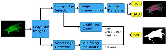
2.3. Image Processing

To process the actin cytoskeleton images of the control and treated cells, the original RGB images were converted to grayscale where the range of the brightness for each pixel was chosen from 0 to 255 [25]. The brightness of the pixels lower than the average brightness ($n_0$) of the whole image were mandatorily set as zero to remove the background color [26]. To quantify the state of the actin cytoskeleton, the grayscale images were skeletonized using Canny and Sobel edge detection techniques, respectively. The actin cytoskeleton was then detected by applying Hough transform to the Canny skeletonized image.

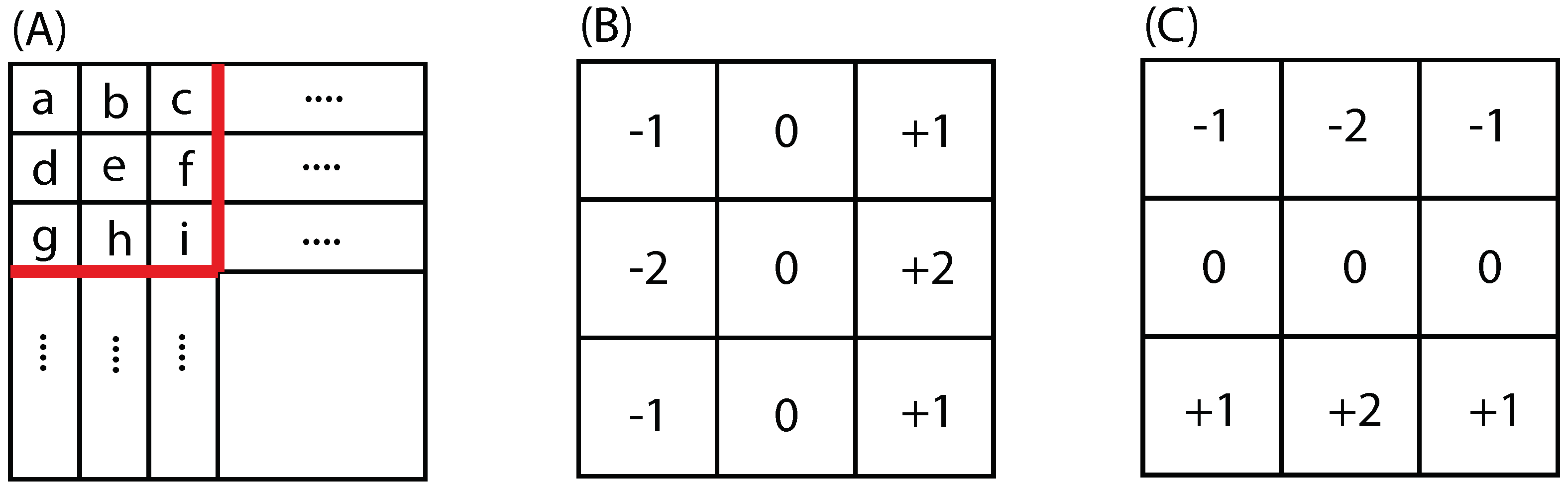
2.3.1. Sobel Edge Detector

The Sobel edge detector performs a two-dimensional gradient measurement on an image and then extracts the boundary information using a threshold applied to the gradient intensity [24]. A pair of convolution masks (as shown in Figure 1) was used in evaluating the gradient measurement in the x-direction and the y-direction, respectively. The convolution mask slides over the input image and changes the value of pixels using 2-dimensional signal processing convolution operation [27]. The magnitude of the gradient was then quantified as,

$$G=\sqrt{{G_x}^2+{G_y}^2}$$

(1)

and,

$$G_x=\left[\begin{array}{ccc}-1& 0& +1\\ -2& 0& +2\\ -1& 0& +1\end{array}\right]★A$$

(2)

$$G_y=\left[\begin{array}{ccc}-1& -2& -1\\ 0& 0& 0\\ +1& +2& +1\end{array}\right]★A$$

(3)

where G is the gradient magnitude and $G_x$ and $G_y$ are the gradient in the x-direction and the y-direction, respectively. A is the source image; the matrices are the convolution masks (see Figure 1); and “★” denotes the 2-dimensional signal processing convolution operation. A pixel location is detected as an edge if its value G exceeds a given threshold.

2.3.2. Canny Edge Detector

The Canny edge detector first uses a data filter, e.g., Gaussian filter, to eliminate the noise in the original image, and then, it follows the same steps of Sobel to evaluate the gradient magnitude (see Equation (1)). However, two thresholds called hysteresis are applied in the Canny algorithm as,

$$\left\{\begin{array}{cc}G\ge S_h,\hfill & G\mathrm{is}\mathrm{a}\mathrm{strong}\mathrm{edge}\mathrm{pixel}\hfill \\ S_l\le G<S_h,\hfill & G\mathrm{is}\mathrm{a}\mathrm{weak}\mathrm{edge}\mathrm{pixel}\hfill \\ G<S_l,\hfill & G\mathrm{is}\mathrm{a}\mathrm{suppressed}\mathrm{edge}\mathrm{pixel}\hfill \end{array}\right.$$

(4)

where $S_h$ and $S_l$ are the high and low threshold values, respectively. A pixel location is detected as an edge if its gradient magnitude (G) is a strong edge pixel, or it is a weak edge pixel with a path connected to the strong edge pixel, otherwise it is set to zero.

The Canny edge detector provides better skeletonized actin filaments than Sobel by removing the fluorescent speckles with the Gaussian filter and hysteresis. However, the Sobel edge detector provides a better result of detecting the cell area with more actin speckles than the Canny technique [24]. This comparison is clearly shown in Figure 2. Therefore, Canny and Sobel skeletonized images were used to obtain the deviation and intensity of the cellular actin cytoskeleton, respectively, as mentioned later.

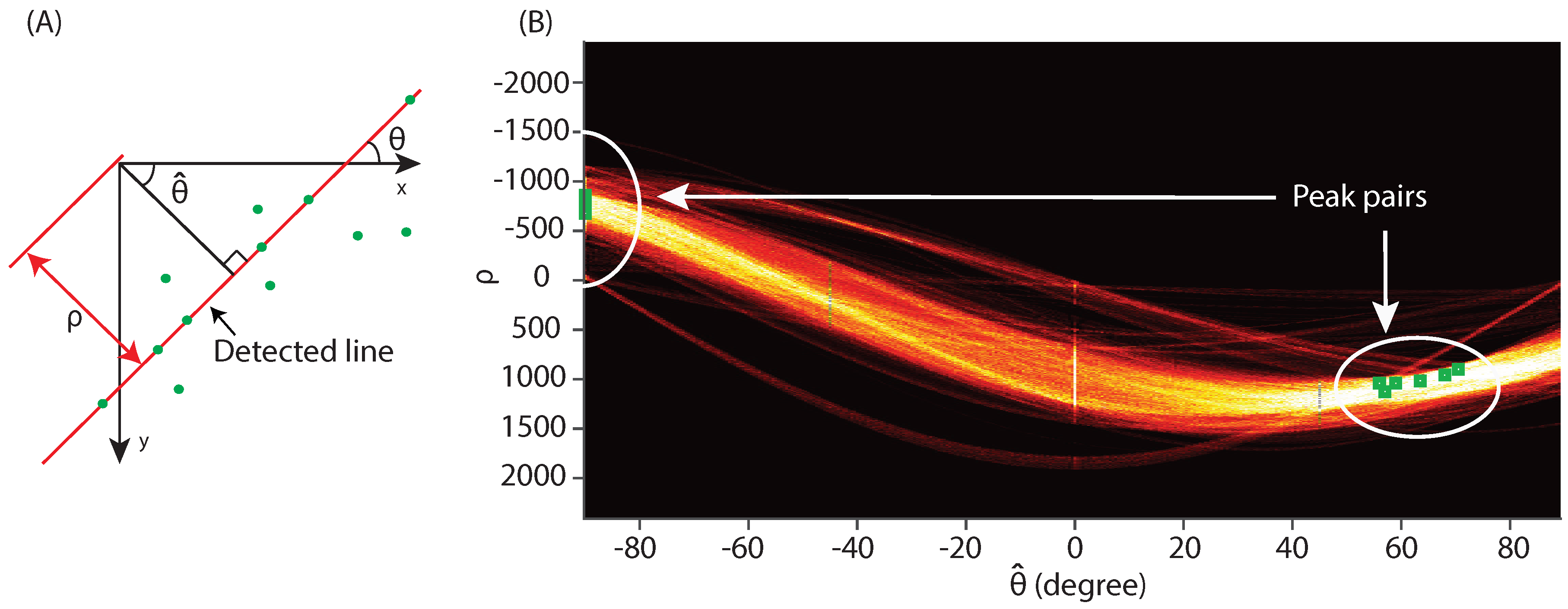
2.3.3. Hough Transform

The actin cytoskeleton was then detected by applying Hough transform to the skeletonized images obtained from the Canny edge detector. Hough transform is a line extraction technique for digital image processing [28]. For each data point in the image, a number of lines with different angles is plotted going through it. For each line, the length ($\rho$, i.e., perpendicular distance to the origin) and the angle ($\widehat{\theta }$) of the perpendicular projection from the pre-chosen origin to the plotted line are measured. Thus, a $\rho$ vs. $\widehat{\theta }$ curve can be plotted for this data point. This curve is then generated repeatedly for each data point and the curves of all the data points together form a Hough space graph (as shown in Figure 3). In the Hough space graph, the intersections of the curves indicate the lines that intersect the image data points being tested. Thus, the intersection associated with k curves indicates a line that goes through k test points on the image. Therefore, by setting a threshold for k, line detection becomes finding the pairs ($\widehat{\theta },\rho$) at which at least k curves intersect; see Figure 3 as an example. Next, the direction of each detected line (i.e., actin filament here) is quantified as,

$$\theta =\widehat{\theta }+{90}^{\circ }$$

(5)

where $\widehat{\theta }$ is the angle of the perpendicular projection from the origin to the line measured in degrees counterclockwise from the positive x-axis, and its range is $-{90}^{\circ }\le \widehat{\theta }<{90}^{\circ }$.

2.4. Actin Cytoskeleton Quantification

It has been observed that both the pattern and quantity of the actin filaments inside the cells could affect and reflect the cellular properties [9]. In our IRAQ approach, the cellular actin cytoskeleton was quantified through three parameters: the partial actin-cytoskeletal deviation (PAD) and the total actin-cytoskeletal deviation (TAD) quantify the orientation distribution of the actin filaments, and the average actin-cytoskeletal intensity (AAI) quantifies the average quantity of the actin filament per detected cell area.

2.4.1. Actin Alignment Deviation

The actin alignment deviation quantifies actin alignment uniformity and consists of the partial actin-cytoskeletal deviation (PAD) and the total actin-cytoskeletal deviation (TAD). To exclude the effect of the cell membrane and achieve more information about the actin cytoskeleton, we proposed to divide the Canny skeletonized image into sub-images. For a demonstration, we divided the images into four sub-images in this study, as an example. Note that the image segmentation is user-defined. The actin cytoskeleton in each sub-image was then detected by Hough transform [28,29].

PAD was defined as the standard deviation of the local cytoskeletal direction in a selected segment, and TAD was defined as the standard deviation of the dominant directions of all selected segments. Specifically, PAD is quantified as,

$$PAD=\sqrt{\frac{{\sum }_{i=1}^{N_1}{({\theta }_{ij}-{\theta }_j)}^2}{N_1}}$$

(6)

where ${\theta }_{ij}$ represents the alignment angle of the line i detected in the segment j using the Hough transform, ${\theta }_j$ is the average alignment angle of the lines detected in the segment j, and $N_1$ is the number of detected lines in segment j. TAD is quantified as,

$$TAD=\sqrt{\frac{{\sum }_{j=1}^{N_2}{({\theta }_j-\overline{\theta })}^2}{N_2}}$$

(7)

where $N_2$ is the number of selected segments, and $\overline{\theta }$ represents the average angle of all the selected segments. Therefore, PAD and TAD could represent the bundling and distribution of the actin cytoskeleton in the local cell area and a whole cell, respectively.

2.4.2. Actin Intensity

Average actin intensity (AAI) is calculated to quantify the quantity and intensity of cellular actin filaments. An actin protein could be presented as either a free monomer called globular-actin (G-actin) or as part of a linear polymer called filamentous-actin (F-actin) [8]. Although phalloidin used to stain the cells was only able to bind to F-actin, nonspecific staining may occur and show in the images [30]. To eliminate the nonspecific staining effect, a pixel count vs. brightness curve is generated first. Specifically, the count and brightness of pixels are generated using the histogram, a representation of the distribution of numerical data, of the Canny skeletonized image with the bin of 1. Then, the summational (i.e., total) intensity (i.e,. brightness in actin cytoskeleton images) from the first local minimal of brightness ($n_1$) to the maximum brightness ($n_2$) of the pixel count vs. brightness curve, ${\sum }_{n=n_1}^{n_2}n\times c$ (see Equation (8)) is treated as the total intensity of the actin filaments, and the average actin-cytoskeletal intensity (AAI) is quantified as,

$$AAI=\frac{{\sum }_{n=n_1}^{n_2}n\times c}{A}$$

(8)

where c is the count of pixels with brightness n and A is the area of the target cell quantified using Sobel edge detection [31] together with an image-filling tool, e.g., hole-filling and line-dilation operations [32].

The entire process of IRAQ is summarized in Figure 4.

2.5. Statistical Analysis

The data in the figures are presented as the mean ± SD. Student’s t-test was performed to evaluate statistical significance, and the p-values are reported in the figures.

3. Results and Discussion

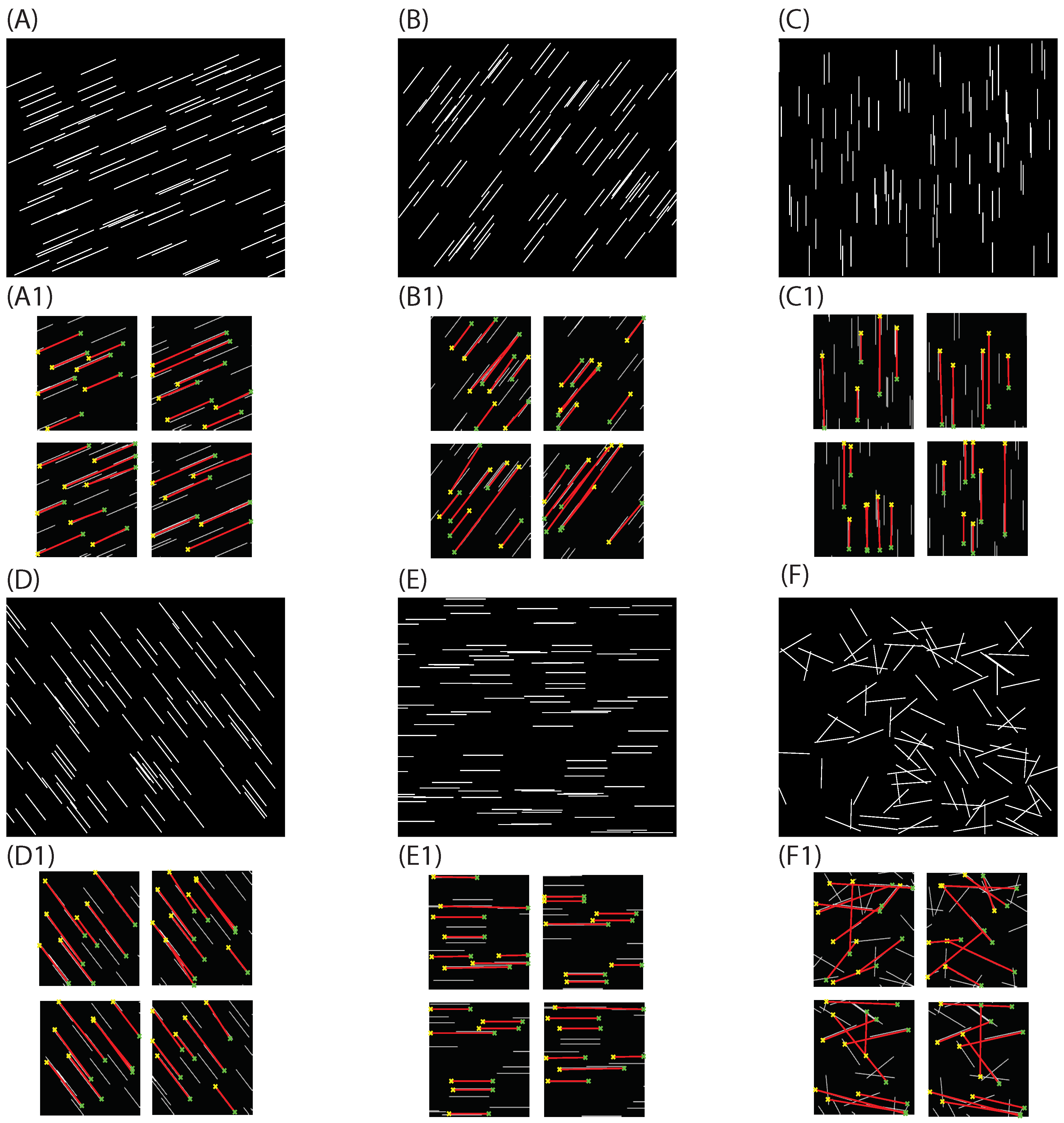
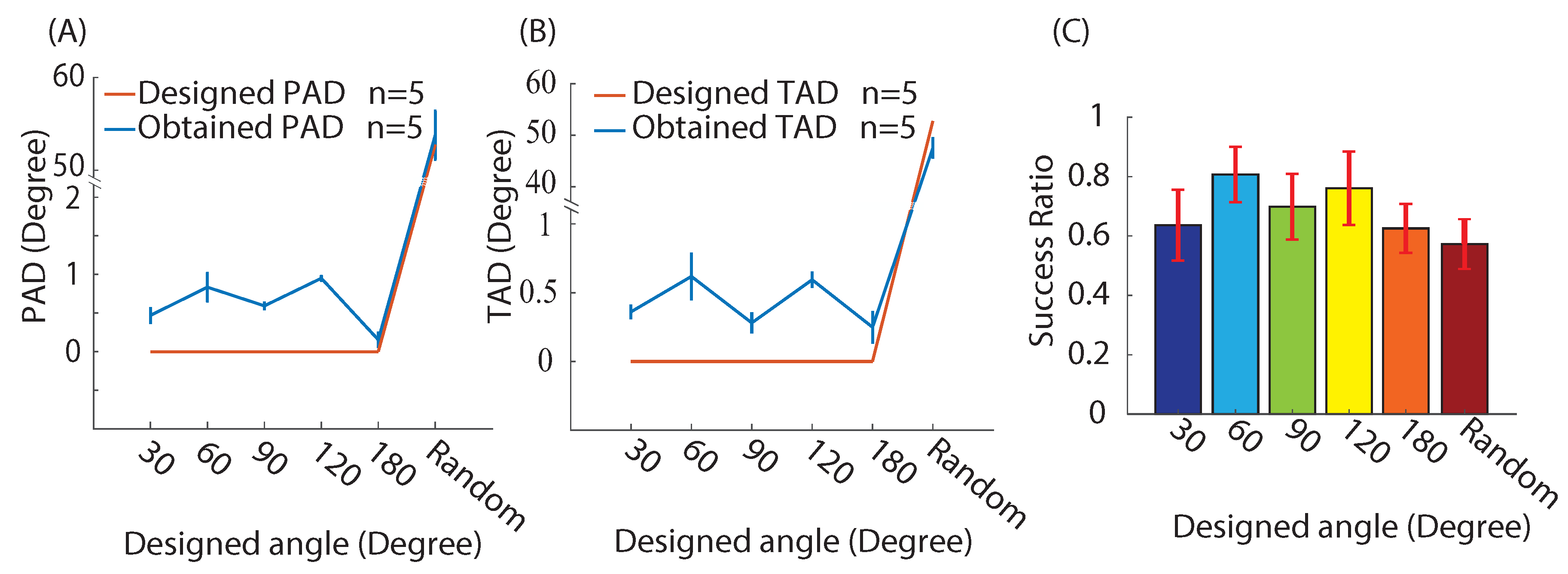
3.1. Approach Validation

For validation first, six different actin cytoskeleton mesh work models were designed in MATLAB to check the quantification accuracy of IRAQ. The models were created in 2D with specified actin alignment angles and angle deviations, as shown in Figure 5. The first five images were created with the actin alignment angles of 30${}^{\circ }$, 60${}^{\circ }$, 90${}^{\circ }$, 120${}^{\circ }$, 180${}^{\circ }$, respectively, and their standard deviations were all 0${}^{\circ }$. The last model was created with random alignment angles, but with the specified standard deviation of 52.75${}^{\circ }$. Five images were created for each model, and for each image, four different segments ($N_2$) were chosen to detect the actin alignment angles. The partial actin-cytoskeletal deviation (PAD) and the total actin-cytoskeletal deviation (TAD) were then quantified according to the aforementioned approach (see Figure 5), and the quantification results are shown in Figure 6A,B and compared to the designed values. Moreover, the IRAQ line detection success ratio (detected line numbers vs. the desired line numbers) are also shown in Figure 6C for validation, as well.

As shown in Figure 6A,B, the average error between the quantified PAD and the designed PAD of all six models was less than 0.67${}^{\circ }$, and the quantified TAD was less than 1.22${}^{\circ }$ different from the designed TAD for all six models. Moreover, the successful detection ratios of the designed models (30${}^{\circ }$, 60${}^{\circ }$, 90${}^{\circ }$, 120${}^{\circ }$, 180${}^{\circ }$) were all larger than 0.63, and that of the random model was larger than 0.57. Note that the line detection success ratio was closely related to the thresholds used in the Hough transform line detector. The bigger the threshold range was, the greater the numbers of lines that can be detected. Thus, by comparing the quantification results with the designed deviation values, the obtained PAD and TAD match the designed values fairly well. Therefore, the proposed image processing approach is quite accurate.

3.2. Actin Cytoskeleton Quantification

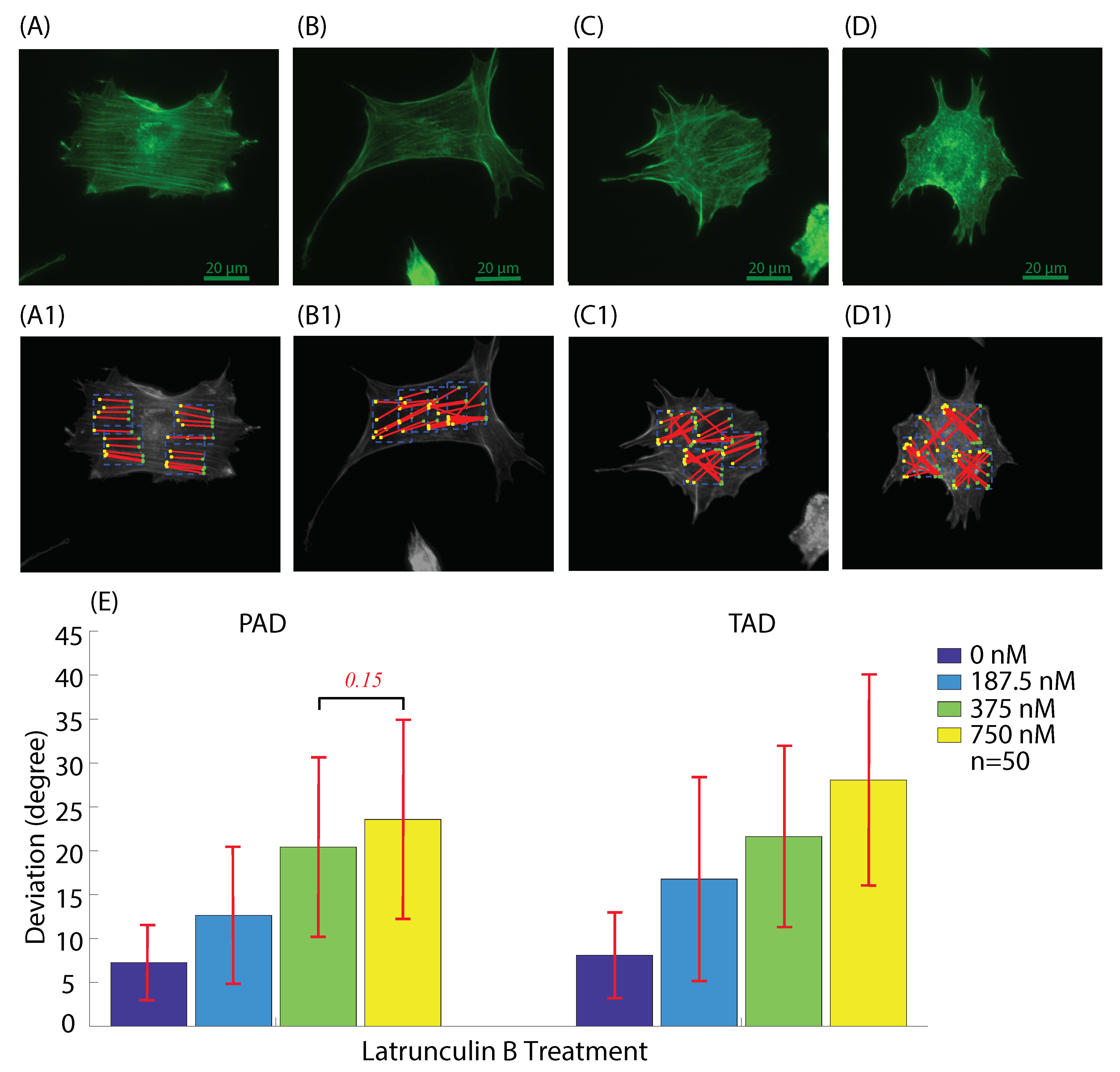
3.2.1. Actin Deviation

After validation, the proposed IRAQ approach was then applied to quantify the actin cytoskeleton of NIH/3T3 cells. To quantify the cell actin cytoskeleton, the images of fifty untreated cells (i.e., treatment concentration of 0 nM) and fifty latrunculin B (F-actin inhibitor) treated cells for each treatment condition (i.e., latrunculin B concentration of 187.5 nM, 375 nM, and 750 nM) were taken using a fluorescence microscope. The images were skeletonized using Canny edge detection, and Hough transform was then applied to detect the F-actin (i.e., lines) of the actin cytoskeleton, as mentioned before. For both untreated and treated cell images, four different segments around the nucleus were chosen to detect the direction of the actin cytoskeleton. PAD and TAD were then calculated according to Equations (6) and (7), respectively. The results are shown in Figure 7.

According to the results, PAD = 7 ± 4 ${}^{\circ }$ and TAD = 8 ± 5${}^{\circ }$ were obtained for the untreated cells, both of which were smaller than PAD = 13 ± 8${}^{\circ }$ and TAD = 17 ± 12${}^{\circ }$, PAD = 20 ± 10${}^{\circ }$ and TAD = 22 ± 10${}^{\circ }$, PAD = 24 ± 12${}^{\circ }$ and TAD = 28 ± 12${}^{\circ }$ of the treated cells with the treatment concentration of 187.5 nM, 375 nM, and 750 nM, respectively. This reduction of TAD and PAD indicates that both the local and total actin-cytoskeletal organization became more disordered with the increase of the latrunculin B concentration. More specifically, both PAD and TAD increased monotonically with the increase of latrunculin B concentration. This observation is consistent with previous studies on other cell types, which have shown qualitatively that the actin filaments are disrupted and replaced by large focal aggregates of F-actin with the increase of latrunculin concentration [10,33]; however, a more quantitative comparison is provided using the proposed IRAQ in this study. Indeed, the actin cytoskeleton was disrupted by latrunculin B through sequestering the globular-actin and blocking the polymerization of the actin filaments [10], which led to the “random”-like alignment of the actin cytoskeleton. As studies have shown, the organization difference of actin filaments between the untreated and treated cells results in the difference of the mechanical properties of the cells [34]; thus, the actin deviation could be applied as a parameter to quantify the cellular mechanical properties in further research.

To further study how latrunculin B affects the organization of the actin cytoskeleton, we measured the actin intensity of the cells treated with different latrunculin B doses and the control (untreated cells).

3.2.2. Actin Intensity

To quantify the average actin intensity (AAI) of the untreated and treated cells, the quantification operation was repeated fifty times (each time on a different cell) for each treatment condition, as shown in Figure 8 and Figure 9.

Based on the cell image intensity distribution result (e.g., Figure 8), $n_1$ = $10\pm 2$ and $n_2$ = 96 ± 30 were quantified for the untreated cells;while $n_1$ = $10\pm 2$ and $n_2$ = $87\pm 26$, $n_1$ = $10\pm 2$ and $n_2$ = $83\pm 28$, $n_1$ = $9\pm 2$ and $n_2$ = $87\pm 25$ were yielded in the quantification of the treated cells with treatment concentration of 187.5 nM, 375 nM, and 750 nM, respectively. Compared with the range of the brightness (0∼255), the error of $n_1$ and $n_2$ was 0.26% and 5.18%, respectively. Specifically, the statistical analysis showed that there were no significant changes in either $n_1$ or $n_2$ (p > 0.5). The consistencies in $n_1$ and $n_2$ for all images (for all treated and untreated cells) reflect that the brightness range (i.e., fluorescence concentrations) of the untreated and treated cells images was essentially the same. In other words, the actin cytoskeleton images were taken under similar conditions (e.g., light intensity and exposure time). The total cell brightness (see Equation (8)) of the untreated cells was $3\pm 2\times {10}^6$ with A = 7 ± 4 × ${10}^3$ $\mathsf{\mu }$m${}^2$; however, for the latrunculin B-treated cells with the concentrations of 187.5 nM, 375 nM, and 750 nM, the total brightness was 2 ± 2 × ${10}^6$ with A = 7 ± 4 × ${10}^3$ $\mathsf{\mu }$m${}^2$, 2 ± 1 × ${10}^6$ with A = $5\pm 3$ × ${10}^3$ $\mathsf{\mu }$m${}^2$, and 2 ± 1 × ${10}^6$ with A = $5\pm 3$ × ${10}^3$ $\mathsf{\mu }$m${}^2$, respectively, with a significant change at higher treatment concentrations (i.e., 375 nM and 750 nM) compared to untreated cells (Figure 9).

AAI were then evaluated (see Equation (8)) as $423\pm 96/\mathsf{\mu }$m${}^2$, $371\pm 74/\mathsf{\mu }$m${}^2$, $356\pm 82/\mathsf{\mu }$m${}^2$, and $348\pm 54/\mathsf{\mu }$m${}^2$ for the cells with treatment concentrations of 0 nM (untreated cells), 187.5 nM, 375 nM, and 750 nM, respectively, as shown in Figure 9. Specifically, the AAI of treated cells changed dramatically compared with the untreated cells (p < 0.05). Clearly, the total cell brightness was decreasing with the increase of the treatment concentration, which indicates that the actin cytoskeleton (with lower brightness in the treated cells) was depolymerized due to the latrunculin B treatment, and the depolymerization degree increased monotonically with the treatment concentration. Moreover, the reduction of the detected cell area showed that latrunculin B also caused the cell area to shrink, and this phenomenon was more pronounced for cells treated with a higher latrunculin B concentration. This observation is also consistent with the previous findings that the actin filament depolymerization caused by latrunculin B could weaken the cell spreading ability [10,35]. Moreover, the reduction of AAI demonstrates that the quantity of the actin cytoskeleton per unit cell area decreased significantly because of the latrunculin B treatment, which means the depolymerization of the actin filaments is more significant compared to the cell area shrinkage under latrunculin B treatment.

3.3. Quantification Result Comparison

To validate the proposed IRAQ approach, the FiberScore algorithm [2] was applied to the same aforementioned F-actin images to quantify the total FiberScore (TF, i.e., the total brightness), the partial deviation (PD), and the total deviation (TD) of F-actin orientation. The quantification results are shown in Figure 10.

Although the results have shown the total FiberScore (i.e., the total F-actin brightness) of the untreated cells was higher than the treated cells, no significant difference was detected from the cells treated with different latrunculin B concentrations. On the contrary, all of the F-actin cell area, total cell brightness, and AAI quantified in IRAQ (see Figure 10) showed a clear monotonically decreasing relation between the F-actin quantity (i.e., fluorescent intensity) and the latrunculin treatment concentrations. This demonstrates that the proposed IRAQ was more sensitive than the reported FiberScore algorithm [2] for fluorescent F-actin intensity quantification. Meanwhile, since the orientation angles were quantified per detected pixel group, the FiberScore algorithm could not detect the F-actin orientation difference for any of the tested cells (both untreated and treated ones). Particularly, both the partial deviation and total deviation yielded no significant difference between the cell treatment under either of the two conditions (see Figure 10). However, both the PAD and TAD quantified in IRAQ (see Figure 9) showed that the F-actin cytoskeleton became significantly more disordered as the latrunculin B dosage was increased. Moreover, the changes of F-actin orientation and quantity due to different latrunculin B treatment dosages are clearly shown in the F-actin fluorescence images. Therefore, it is clear that the proposed IRAQ is quite sensitive to detecting the F-actin cytoskeleton change, and the comparison indicated that IRAQ can be reliably used in further research to study the quantitative relation between the actin cytoskeleton morphology and the cellular mechanical properties, as previous studies have shown that latrunculin B treatment tends to alter the cell mechanical properties significantly [9,10,11,12].

Note that although the actin cytoskeleton was quantified in this study for demonstration, IRAQ can also be implemented for quantification of other 2D cellular structures by adopting proper pattern detection algorithms as long as clear optical images of the corresponding cell structures are accessible. One limitation of the proposed IRAQ is that the alignment and intensity quantification results are closely related to the threshold values used in the Sobel and Canny edge detectors, respectively. One possible improvement that can be made is to implement an automatic threshold tuning process in order to increase the detection sensitivity of the proposed IRAQ. To understand the cell mechanotransduction dynamics fully, the IRAQ approach may be further implemented for quantitative studies of the correlation between cytoskeleton structure and physiological and biomechanical behavior of the cells affected by the change of the cellular cytoskeleton structure. As for the future work, the IRAQ approach will be extended to the quantification of cells with different cytoskeleton structures caused by multiple treatment drugs. Furthermore, cells’ physiological and biomechanical properties will be analyzed and explained according to the change of different cellular cytoskeletons.

4. Conclusions

In this study, an image recognition-based actin cytoskeleton quantification (IRAQ) approach is proposed. It is proposed to quantify the actin cytoskeleton using three parameters: the partial actin-cytoskeletal deviation (PAD) and the total actin-cytoskeletal deviation (TAD) quantify the orientation distribution of the actin filaments, and the average actin-cytoskeletal intensity (AAI) quantifies the average quantity of the actin filaments per detected cell area. IRAQ was validated through quantification of artificially-generated actin cytoskeleton models, and the quantified results of the proposed approach matched the designed values very well. To demonstrate the contribution of this work, IRAQ was then applied to quantify the actin cytoskeleton state of NIH/3T3 cells treated with latrunculin B. The quantified results of PAD and TAD quantitatively showed that the local and total actin-cytoskeletal organization of the treated cells were more disordered for the cells treated with a higher concentration, and the disorderliness was increasing with the increase of the treatment concentration. The AAI values suggested that the quantity of the actin cytoskeleton was decreasing monotonically with the latrunculin B treatment concentration increase. As the actin cytoskeleton state is closely related to cellular mechanical behavior dynamics, IRAQ can be implemented for quantitative studies of the correlation between cytoskeleton structure and cell mechanotransduction dynamics.

References

1. Elosegui-Artola, A.; Jorge-Peñas, A.; Moreno-Arotzena, O.; Oregi, A.; Lasa, M.; García-Aznar, J.M.; De Juan-Pardo, E.M.; Aldabe, R. Image analysis for the quantitative comparison of stress fibers and focal adhesions. PLoS ONE 2014, 9, e107393. [Google Scholar] [CrossRef] [PubMed]
2. Lichtenstein, N.; Geiger, B.; Kam, Z. Quantitative analysis of cytoskeletal organization by digital fluorescent microscopy. Cytom. Part A 2003, 54, 8–18. [Google Scholar] [CrossRef] [PubMed] [Green Version]
3. Mollaeian, K.; Liu, Y.; Ren, J. Investigation of Nanoscale Poroelasticity of Eukaryotic Cells Using Atomic Force Microscopy. In Proceedings of the ASME 2017 Dynamic Systems and Control Conference American Society of Mechanical Engineers, Tysons, VI, USA, 11–13 October 2017; p. V001T08A005. [Google Scholar]
4. Alioscha-Perez, M.; Benadiba, C.; Goossens, K.; Kasas, S.; Dietler, G.; Willaert, R.; Sahli, H. A robust actin filaments image analysis framework. PLoS Comput. Biol. 2016, 12, e1005063. [Google Scholar] [CrossRef] [PubMed]
5. Weichsel, J.; Urban, E.; Small, J.V.; Schwarz, U.S. Reconstructing the orientation distribution of actin filaments in the lamellipodium of migrating keratocytes from electron microscopy tomography data. Cytom. Part A 2012, 81, 496–507. [Google Scholar] [CrossRef] [PubMed] [Green Version]
6. Mollaeian, K.; Liu, Y.; Bi, S.; Ren, J. Atomic force microscopy study revealed velocity-dependence and nonlinearity of nanoscale poroelasticity of eukaryotic cells. J. Mech. Behav. Biomed. Mater. 2018, 78, 65–73. [Google Scholar] [CrossRef]
7. Tamiello, C.; Buskermolen, A.B.; Baaijens, F.P.; Broers, J.L.; Bouten, C.V. Heading in the right direction: Understanding cellular orientation responses to complex biophysical environments. Cell. Mol. Bioeng. 2016, 9, 12–37. [Google Scholar] [CrossRef]
8. Pullarkat, P.A.; Fernández, P.A.; Ott, A. Rheological properties of the eukaryotic cell cytoskeleton. Phys. Rep. 2007, 449, 29–53. [Google Scholar] [CrossRef]
9. Gupta, M.; Sarangi, B.R.; Deschamps, J.; Nematbakhsh, Y.; Callan-Jones, A.; Margadant, F.; Mège, R.M.; Lim, C.T.; Voituriez, R.; Ladoux, B. Adaptive rheology and ordering of cell cytoskeleton govern matrix rigidity sensing. Nat. Commun. 2015, 6, 7525. [Google Scholar] [CrossRef] [Green Version]
10. Wakatsuki, T.; Schwab, B.; Thompson, N.C.; Elson, E.L. Effects of cytochalasin D and latrunculin B on mechanical properties of cells. J. Cell Sci. 2001, 114, 1025–1036. [Google Scholar] [PubMed]
11. Sims, J.R.; Karp, S.; Ingber, D.E. Altering the cellular mechanical force balance results in integrated changes in cell, cytoskeletal and nuclear shape. J. Cell Sci. 1992, 103, 1215–1222. [Google Scholar]
12. Mollaeian, K.; Liu, Y.; Bi, S.; Wang, Y.; Ren, J.; Lu, M. Nonlinear Cellular Mechanical Behavior Adaptation to Substrate Mechanics Identified by Atomic Force Microscope. Int. J. Mol. Sci. 2018, 19, 3461. [Google Scholar] [CrossRef]
13. Kimori, Y.; Hikino, K.; Nishimura, M.; Mano, S. Quantifying morphological features of actin cytoskeletal filaments in plant cells based on mathematical morphology. J. Theor. Biol. 2016, 389, 123–131. [Google Scholar] [CrossRef] [PubMed]
14. Kunttu, I.; Lepistö, L.; Rauhamaa, J.; Visa, A. Multiscale Fourier descriptors for defect image retrieval. Pattern Recognit. Lett. 2006, 27, 123–132. [Google Scholar] [CrossRef]
15. Liu, Y.; Mollaeian, K.; Ren, J. Finite element modeling of living cells for AFM indentation-based biomechanical characterization. Micron 2018. [Google Scholar] [CrossRef]
16. Patel, M.N.; Tandel, P. A Survey on Feature Extraction Techniques for Shape based Object Recognition. Int. J. Comput. Appl. 2016, 0975–8887. [Google Scholar]
17. Castañón, C.A.; Fraga, J.S.; Fernandez, S.; Gruber, A.; Costa, L.d.F. Biological shape characterization for automatic image recognition and diagnosis of protozoan parasites of the genus Eimeria. Pattern Recognit. 2007, 40, 1899–1910. [Google Scholar] [CrossRef]
18. Takamatsu, A.; Takaba, E.; Takizawa, G. Environment-dependent morphology in plasmodium of true slime mold Physarum polycephalum and a network growth model. J. Theor. Biol. 2009, 256, 29–44. [Google Scholar] [CrossRef]
19. Pantic, I.; Harhaji-Trajkovic, L.; Pantovic, A.; Milosevic, N.T.; Trajkovic, V. Changes in fractal dimension and lacunarity as early markers of UV-induced apoptosis. J. Theor. Biol. 2012, 303, 87–92. [Google Scholar] [CrossRef] [PubMed]
20. Verkhovsky, A.B.; Chaga, O.Y.; Schaub, S.; Svitkina, T.M.; Meister, J.J.; Borisy, G.G. Orientational order of the lamellipodial actin network as demonstrated in living motile cells. Mol. Biol. Cell 2003, 14, 4667–4675. [Google Scholar] [CrossRef]
21. Higaki, T.; Kutsuna, N.; Sano, T.; Kondo, N.; Hasezawa, S. Quantification and cluster analysis of actin cytoskeletal structures in plant cells: Role of actin bundling in stomatal movement during diurnal cycles in Arabidopsis guard cells. Plant J. 2010, 61, 156–165. [Google Scholar] [CrossRef]
22. Basu, S.; Liu, C.; Rohde, G.K. Localizing and extracting filament distributions from microscopy images. J. Microsc. 2015, 258, 13–23. [Google Scholar] [CrossRef] [PubMed]
23. Tondon, A.; Kaunas, R. The direction of stretch-induced cell and stress fiber orientation depends on collagen matrix stress. PLoS ONE 2014, 9, e89592. [Google Scholar] [CrossRef] [PubMed]
24. Vijayarani, S.; Vinupriya, M. Performance analysis of canny and sobel edge detection algorithms in image mining. Int. J. Innov. Res. Comput. Commun. Eng. 2013, 1, 1760–1767. [Google Scholar]
25. Ojala, T.; Pietikainen, M.; Maenpaa, T. Multiresolution gray-scale and rotation invariant texture classification with local binary patterns. IEEE Trans. Pattern Anal. Mach. Intell. 2002, 24, 971–987. [Google Scholar] [CrossRef] [Green Version]
26. Wang, Y.; Chen, Q.; Zhang, B. Image enhancement based on equal area dualistic sub-image histogram equalization method. IEEE Trans. Consum. Electron. 1999, 45, 68–75. [Google Scholar] [CrossRef]
27. Feibush, E.A.; Levoy, M.; Cook, R.L. Synthetic texturing using digital filters. In ACM SIGGRAPH Computer Graphics; ACM: New York, NY, USA, 1980; Volume 14, pp. 294–301. [Google Scholar]
28. Ballard, D.H. Generalizing the Hough transform to detect arbitrary shapes. In Readings in Computer Vision; Elsevier: Amsterdam, The Netherlands, 1987; pp. 714–725. [Google Scholar]
29. Liu, Y.; Ren, J. Modeling and Control of Dynamic Cellular Mechanotransduction (I): Actin Cytoskeleton Quantification; ASME: New York, NY, USA, 2018. [Google Scholar]
30. Cooper, J.A. Effects of cytochalasin and phalloidin on actin. J. Cell Biol. 1987, 105, 1473–1478. [Google Scholar] [CrossRef] [Green Version]
31. Maini, R.; Aggarwal, H. Study and comparison of various image edge detection techniques. Int. J. Image Process. 2009, 3, 1–11. [Google Scholar]
32. Baxes, G.A. Digital Image Processing: Principles and Applications; Wiley: New York, NY, USA, 1994. [Google Scholar]
33. Bear, J.E.; Svitkina, T.M.; Krause, M.; Schafer, D.A.; Loureiro, J.J.; Strasser, G.A.; Maly, I.V.; Chaga, O.Y.; Cooper, J.A.; Borisy, G.G.; et al. Antagonism between Ena/VASP proteins and actin filament capping regulates fibroblast motility. Cell 2002, 109, 509–521. [Google Scholar] [CrossRef]
34. Wang, S.; Arellano-Santoyo, H.; Combs, P.A.; Shaevitz, J.W. Actin-like cytoskeleton filaments contribute to cell mechanics in bacteria. Proc. Natl. Acad. Sci. USA 2010, 107, 9182–9185. [Google Scholar] [CrossRef] [Green Version]
35. Chen, T.; Teng, N.; Wu, X.; Wang, Y.; Tang, W.; Šamaj, J.; Baluška, F.; Lin, J. Disruption of actin filaments by latrunculin B affects cell wall construction in Picea meyeri pollen tube by disturbing vesicle trafficking. Plant Cell Physiol. 2007, 48, 19–30. [Google Scholar] [CrossRef]
Figure 1. Gradient measurement in the Sobel edge detector: (A) the original image with the evaluated brightness in each pixel; (B,C) are the convolution masks in the x-direction and the y-direction, respectively.
Electronics 07 00443 g001
Figure 2. Image skeletonization: (A) the converted fixed-cell image of an untreated cell in grayscale; (B,C) are the skeletonized image of (A) using Sobel and Canny edge detectors, respectively.
Electronics 07 00443 g002
Figure 3. Illustrative demonstration of Hough transform: (A) line detection process. The green points are the bright pixels on the skeletonized actin cytoskeleton images. The red line is detected based on the green points. θ ^ is the angle of the perpendicular projection from the origin to the detected line measured in degrees anticlockwise from the positive x-axis. ρ is the distance between the origin and the detected line. The ( θ ^ , ρ ) pair is given by Hough transform. θ calculated through θ ^ is the angle of the detected line. (B) Hough space graph of the Canny skeletonized image in Figure 2C. The green points are the ( θ ^ , ρ ) pairs at which at least 10 curves intersect.
Electronics 07 00443 g003
Figure 4. Quantification process of the proposed image recognition-based actin cytoskeleton quantification (IRAQ). PAD, partial actin-cytoskeletal deviation; TAD, total actin-cytoskeletal deviation (TAD); AAI, average actin-cytoskeletal intensity.
Electronics 07 00443 g004
Figure 5. Artificially created actin cytoskeleton images with the F-actin alignment angles of: (A) 30 ; (B) 60 ; (C) 90 ; (D) 120 ; (E) 180 ; and (F) random with a standard deviation of 52.75 . PAD and TAD of models (AE) are all 0 , and 52.75 for model (F); (A1F1) are the line detection results of the four selected segments of the models (AF), respectively.
Electronics 07 00443 g005
Figure 6. The alignment quantification result of (A) PAD and (B) TAD. The F-actin alignment deviation (red line) of models with orientation angles of 30 ∼180 are 0 , and the alignment deviation is 52.75 for the random orientation model. The blue line denotes the quantified deviation of the successfully-detected F-actin filaments. The average error between the quantified PAD and the designed PAD of all six models was less than 0.67 , and it was less than 1.22 between the quantified and designed TAD. (C) The line detection success ratio (i.e., the number of IRAQ detected lines vs. original line numbers) for each model.
Electronics 07 00443 g006
Figure 7. Example actin cytoskeleton images of cells with latrunculin B treatment concentration of: (A) 0 nM; (B) 187.5 nM; (C) 375 nM; (D) 750 nM; (A1D1) are the line detection result of the actin cytoskeleton in the four segments randomly selected from (AD), respectively. (E) The quantification results of PAD and TAD. PAD = 7 ± 4 and TAD = 8 ± 5 for 0 nM (untreated cells); PAD = 13 ± 8 and TAD = 17 ± 12 , PAD = 20 ± 10 and TAD = 22 ± 10 , PAD = 24 ± 12 and TAD = 28 ± 12 ; for the treatment concentrations of 187.5 nM, 375 nM, and 750 nM, respectively. n = 50. Student’s t-test was performed to analyze the statistical difference: the F-actin alignment deviation obtained from each treatment condition was compared with respect to that from the other three treatments. A p < 0.05 was yielded for each comparison, unless otherwise denoted in the figure (with p-values in red italic font).
Electronics 07 00443 g007
Figure 8. Example actin cytoskeleton images of cells with latrunculin B treatment concentrations of: (A) 0 nM; (B) 187.5 nM; (C) 375 nM; (D) 750 nM; (A1D1) are the detected cell area of (AD) using the Sobel edge detector and the hole-filling tool, respectively; (A2D2) are the brightness distribution of (AD), respectively. The blue curves denote the count of pixels at each specific brightness; the orange curves are the fitting result of its distribution; the circle denotes the first minimal intensity of the fitting result.
Electronics 07 00443 g008
Figure 9. F-actin cytoskeleton intensity quantification result for each treatment condition: (A) the minimum brightness ( n 1 ) and maximum brightness ( n 2 ); (B) the total cell brightness; (C) the detected F-actin cell area; and (D) average actin intensity (AAI), respectively. For the untreated cells, AAI = 423 ± 96/ μ m 2 , and the treated cell had AAI = 371 ± 74 / μ m 2 , AAI = 356 ± 82 / μ m 2 , and AAI = 348 ± 54 μ m 2 for the treatment concentrations of 187.5 nM, 375 nM, and 750 nM, respectively. n = 50. Student’s t-test was performed to analyze the statistical difference: the quantification results obtained from each treatment condition were compared with respect to that from other three treatments, respectively. A p < 0.05 was yielded for each comparison, unless otherwise denoted in the figure (with p-values in red italic font). NS: not significant.
Electronics 07 00443 g009
Figure 10. The FiberScore algorithm quantification result for each latrunculin B treatment condition: (A) total FiberScore (TF); (B) partial deviation (PD) and total deviation (TD). For the untreated cells, TF = 8800 ± 5800, PD = 50 ± 5, and TD = 50 ± 5, and the treated cells have TF = 7000 ± 3700, PD = 51 ± 5, and TD = 51 ± 5, TF = 6600 ± 4600, PD = 51 ± 6, and TD = 50 ± 6, and TF = 6600 ± 4200, PD = 50 ± 6, and TD = 50 ± 6 for the treatment concentrations of 187.5 nM, 375 nM, and 750 nM, respectively. n = 50. Student’s t-test was performed to analyze the statistical difference: the quantification results obtained from each treatment condition were compared with respect to that from the other three treatments, respectively. A p < 0.05 was yielded for each comparison, unless otherwise denoted in the figure (with p-values in red italic font). NS: not significant.
Electronics 07 00443 g010