Abstract
This work is concerned with the mechanical design and the description of the different components of a new mobile base for a lightweight mobile manipulator. These kinds of mobile manipulators are normally composed of multiple lightweight links mounted on a mobile platform. This work is focused on the description of the mobile platform, the development of a new kinematic model and the design of a control strategy for the system. The proposed kinematic model and control strategy are validated by means of experimentation using the real prototype. The workspace of the system is also defined.
1. Introduction
When compared to conventional manipulators, lightweight link manipulators have the following advantages: a lower cost, a larger work volume (they have longer links), a higher operational speed, a greater payload-to-manipulator-weight ratio, smaller actuators, less energy consumption, better maneuverability, better transportability and safer operation owing to reduced inertia. These numerous advantages have led to the extensive use of these kind of manipulators in various robotic applications, thus making them of great interest to many researchers throughout the world over the last few decades. Because energy consumption in motors is directly proportional to the mass and size of robot elements, long and light robot links are commonly used. However, they present the drawbacks of exhibiting vibrations and permanent deflections because of the flexibility of their links. A survey on the mechanics and dynamics of these robots is [1], a survey on their control is [2] and a recent review about of the control and sensor systems of these manipulators is [3].
Mobile manipulators have recently received considerable attention and a wide range of applications have been explored. In most cases, a mobile robot must be capable of some form of manipulation in order to be useful and manipulators are, therefore, mounted on mobile platforms. An extensive literature survey on mobile manipulator systems can be found in [4].
These manipulators usually have power on board with limited energy owing to the difficulty involved in storing a great amount of energy in batteries. This, therefore, makes it necessary to incorporate light links in order to decrease energy consumption. Another important advantage of using lightweight manipulators is that their lightweight features allow longer links to be designed in order to extend the workspace of the manipulators, thus enabling them to reach targets that were, initially, outside their workspace. Some works about the analysis and design of lightweight manipulators mounted on mobile platforms can be found in [5,6], and about trajectory planning of these systems in [7].
Many existing applications take advantage of using arms with lightweight links mounted on mobile platforms. Some of these are: intervention robots, robots used to clean up hazardous waste, for bomb disposal and refighting, the maintenance of dangerous items (e.g., hot electric power lines), or mining robots. For example, Ref. [8] presents a robot to assist humanitarian demining and [9] a design of an automatic system for aircraft painting.
In the context of a multiple large link manipulators mounted on a mobile platform, the movement of the links will reduce the physical stability of the system, increasing the possibilities of overturning of the mobile platform. When the mass of the flexible manipulator is important in comparison with the overall mass of the mobile platform, the center of mass is shifted from the base of the robot. This reduces the maximum speed and the maximum terrain inclination in which the robot can navigate and the maneuvers that the manipulator can perform without leading the center of mass out of the support polygon, finally causing the overturning of the robot. For that reason, four legs have been added to the mobile platform in order to increase the polygon support of the system and increase considerably the physical stability of the system.
In this work, a mechanical device capable of transporting large lightweight manipulators is presented. Its main objectives are: (a) transport the manipulator, (b) increase the stability of the system when it reaches a specific target and (c) help in the positioning of the tip of the manipulator. The innovations introduced in our mechanism over previous designs are related to the inclusion of the four controlled legs in the mobile platform: (1) These four legs enlarge the stability polygon, preventing the overturn of the platform in the case that the large lightweight arm placed on it leans excessively. This approach to increase the robot stability has not been done before in this context. (2) Controlling these legs and, by means of them, the inclination of the platform, allows us to accurately position the tip of the manipulator. These positioning movements are of a reduced range, but, since large movements and approximate positioning are carried out by the wheeled mobile platform, the combination of the displacement and inclination of the robot platform may lead to a precise positioning of the robot tip and the reduction of the number of links and actuators of the lightweight arm (which are usually in charge of the precise positioning of the manipulator tip).
The platform of the system has many similarities to the well-known parallel manipulators (PMs). Parallel manipulators typically consist of a moving platform that is connected to a fixed base by a number of kinematic chains (legs). The number of legs is usually at least equal to the number of degrees of freedom (DOF) of the moving platform. Note that, if the number of degrees of freedom is higher than the number of legs, more than one actuator will be needed on some legs in order to have the same number of actuators and degrees of freedom. In the literature, a large number of mechanical designs for parallel robots with 2 to 6 DOF have been proposed (e.g., [10,11,12]). However, a recent study of the mechanical structure shows that approximately 80 % of parallel robots have 3 DOF or 6 DOF. Most 6 DOF parallel robots are based on the Stewart–Gough platform architecture [13,14]. However, six degrees suffer from the disadvantages of having difficult direct kinematics, coupled positions and orientation, and a small workspace. Parallel manipulators with 3-DOF have, therefore, been thoroughly studied in the last decades for some relevant applications [15]. Although most of the 3-DOF parallel manipulators found in literature have three legs, it is possible to build 3-DOF parallel manipulators with more than three legs. The additional legs act as passive legs that provide more stability to the system. A recent work uses a parallel robot to obtain a static balancing condition expressed as a function of the position and orientation of the mobile platform of the system and the actuated prismatic joint [16].
Each leg uses a four-bar mechanism of 1 DOF (degree of freedom) actuated by a linear actuator. Similar mechanisms are used in a pantograph-leg; however, the function is very different. Pantograph-leg mechanisms are assembly of links and joints with the purpose of simulating the walking motion of humans or animals. Mechanical legs have, normally, one or more actuators depending on the complex motion they have to carry out. Simple planar motion can be carried out with a leg pantograph with 1 DOF that is very similar to the system of the legs of the platform described here. Recent works which analyze the design, kinematics and dynamics of these mechanism can be found in [17,18,19].
In this work, a new kinematic model and a new control strategy for the platform of the system are proposed in order to control the posture and the orientation of the system. Other works which use a similar strategy can be found in [20] where a control based on a kinematic model of the system is developed in order to surpass obstacles such as curbs, ramps or staircases while maintaining the seat’s inclination of a wheelchair. This work was the starting point for the development of the kinematic model and the control strategy of our robot, having in common both systems that they move at slow speed, which allows the design of a control strategy based on the kinematics of the system. However, there are important differences between [20] and our work: (a) the kinematic model of [20] is in a plane (2D), whereas ours is a 3D model, (b) our system has the problem that the supporting points of the legs are uncertain, while the supporting points where known in [20] and (c) the control strategy is different because in the work [20] the actuators have only three states (maximum, zero and minimum speed) while ours can provide values of the speed in a continuous range, which allows us to carry out a control based on the inversion of the kinematic model. The development of the kinematic model and the control strategy of this work is therefore original. The starting point of the platform developed in this work is the large lightweight manipulator, designed by us and described in [21], which is mounted on the mobile platform.
Moreover, the workspace of the manipulator is calculated in order to define the range of operation of the system. The main application of this system is for inspection tasks. The inspection tasks may be relevant for improving security and efficiency in many industrial applications. The system has an overview view camera in the tip of the manipulator and while the system is moving from one place to another, the camera is recording everything. However, when the system reaches an area of interest, the system starts working in the second configuration and it is needed to place the tip of the lightweight in particular points in order to focus a particular point of interest. For that reason, it is very important to define the workspace of the system in order to know which targets can be achieved for the system.
The main contributions of this work are: (1) the description of a novel mobile platform prototype which allows for transporting very large lightweight manipulators, (2) the development of a kinematic model of the system, and (3) the proposed control strategy based on the inversion of a novel kinematic model which allows for increasing the physical stability of the system and help in the positioning of the tip of the manipulator.
This paper is organized as follows. Section 2 describes the mechanical design and the components of the system presented in this work. In Section 3, a new kinematic model is proposed and its validation is presented, along with simulated and experimental results. In Section 4, the workspace of the tip of the manipulator of the system is defined. The design methodology to control the linear actuators of the system is presented in Section 5. A new control strategy based on the inverse kinematics of the system is proposed in Section 5. In Section 7, a brief discussion of the results is made. Finally, some conclusions concerning the results are presented in Section 8.
2. Mechanical Design of the Mobile Platform
The system presented in this work is principally composed of a mobile platform and a very lightweight manipulator. The platform consists of a rectangular base with four legs and four wheels (see Figure 1a). The platform described in this work is based on two different configurations in order to carry out two different tasks. The first configuration is when the legs of the system are up and are not in contact with the ground. In this configuration, the legs are not used and the system is used to transport the manipulator from one place to another.
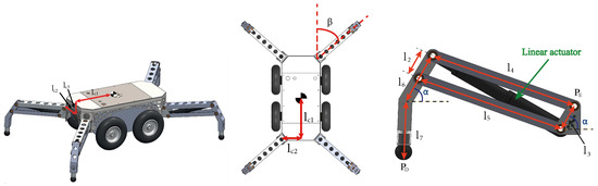
Figure 1.
(a) front view of the mobile platform; (b) top view of the mobile platform; (c) scheme of a leg of the system.
The second configuration is when the legs of the system are in contact with the ground and the wheels are not used. In this case, the system is used to control the orientation and the posture of the base of the manipulator. Moreover, the base is used to increase the static stability of the system because when the mobile platform reaches a particular target, the lightweight manipulator that is on the mobile base will start moving. The legs, therefore, provide a solid base for the system. The purpose of the legs is to improve the stability of the system during the operation of the manipulator, which is above the mobile platform. They provide a solid platform for the safe operation and efficient use of the lightweight manipulator. If the manipulator has to be used, it is important to fully extend all of the legs and to raise the wheels off the ground.
The wheels do not provide the stability needed for the system and the system, therefore, needs the legs to prevent the system from leaning too much to one side or the other, or even from overturning. This is the main purpose of adding four legs to our mobile platform. In the last few decades, mobile cranes have used similar approaches in order to improve their stability. They use support devices called outriggers. The outriggers normally use hydraulics to lift the entire crane, whereas our prototype employs a linear actuator inside a mechanism that can be considered a four-bar mechanism. The legs are used to balance the system and to prevent the system from tipping forward and backward during operation.
Each leg is actuated by a linear actuator which has the function of changing the configuration of the system. Figure 1c shows that modifying the extension of the linear actuator leads to an alteration in the distance between the support point of the leg, , and the point that joins the leg and the base of the truck, , changes.
Figure 1c shows that each leg is a four-bar linkage that consists of four rigid bars in the plane connected by revolute joints. For analytical purposes, four bar linkages are treated as planar mechanisms. However, in practice, the implementation of a four bar linkage could be spatial (non-planar). The four-bar linkage is the simplest and, often, the most useful mechanism. A variety of useful mechanisms can be formed from a four-bar mechanism by making slight variations, such as changing the character of the pairs, proportions of links, etc. As mentioned previously, the objective of the four-bar linkage used in this work is to be able to modify the difference in height between and by modifying the length of the linear actuator, which is located in the middle of the four-bar system. By combining the movement of the four legs, we are, therefore, able to modify the height and the posture (orientation) of the base of the system.

Table 1.
Parameters of the system.
2.1. Components of the Mobile Platform
This section describes the components of the system:
One real-time high-performance embedded controller (NI-PXIe-1082, National Instruments): this is an advanced reconfigurable control and acquisition system. It includes an 8-lot chassis and it runs Labview Real-Time for control and analysis.
Two Modules NI PXIe-6363, National Instruments): this is a multifunction PXI Module. Each module contains 32 analogic inputs, four analogic outputs and 48 digital input-outputs. This module is used to send the control voltage signal to the two motor drivers in order to control the voltage in the linear actuators and to acquire the signal from the accelerometer, the encoders of the linear actuators and the twelve limit switches.
Four linear actuators: linear actuators are electric devices that are able to convert the rotational motion of a DC motor into linear pull/push movements. The con50 (14actuators) are versatile, high efficiency, 12/24V DC industrial motors with planetary gears with small overall dimensions and a very high relation of reduction gear. They are made of powder-coated steel, providing a sturdy design that protects the motor and electric circuits. They are used to control the extension of the legs of the system (see Figure 1c).
Two motor drivers: the Sabertooth 2 × 25 V2 (Dimension Engineering) are very versatile, efficient and easy to use dual motor drivers. The Sabertooth can supply two DC brushed motors with up to 25 A each. On our platform, each Sabertooth allows us to control two linear actuators with analog voltage, independently. They will, therefore, be used to control the position and the direction of the linear actuators.
Four linear actuator encoders: each linear actuator has an encoder that measures the displacement of the linear actuators of the system. These sensors allow us to control the position and the speed of the linear actuators.
Four Maxon DC motor sets: each set is composed of a Maxon DC motor (maxon motor) which is a high-quality motor fitted with powerful permanent magnets. Planetary reduction gears (n = 26) and incremental high precision encoders with high signal resolution are mounted exclusively on motors with through shafts for reasons of resonance. They are used to control the rotational movement of the wheels of the system.
Four Positioning controllers (EPOS2 24/5, maxon motor): these are small smart motion controllers. Owing to the flexible and high efficient power stage, the EPOS 24/5 drives both brushed DC motors with a digital encoder and brushless EC motors with digital Hall sensors and encoders. They integrate position, velocity and current controls, which allow the user to develop sophisticated positioning applications. Each of these controllers is used to move one of the Maxon DC motors.
Twelve limit switches: these switches include electrical contacts with which to energize and de-energize a circuit. Four switches are located in order to detect the maximum extension of each leg and the other four switches are located in order to detect the maximum shrinkage of each leg. These eight switches are used in order to avoid damage to the system when it surpasses its mechanical limits. The system also has four other switches in order to detect when the leg is in contact with the ground. This will be very important when the stabilization process is used.
One inertial sensor: the sensor is called ADIS16448 and is a complete inertial system that includes a triaxial gyroscope, a triaxial accelerometer and a triaxial magnetometer. The sensor has been placed in the central part of the base of the truck in order to measure the orientation of the base of the platform.
Figure 2 shows a scheme of the components of the system.
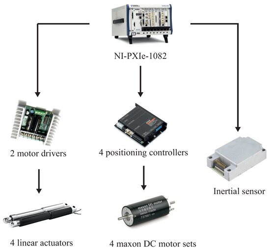
Figure 2.
Components of the platform.
2.2. General Approach of the System
- The system transports the lightweight manipulator in the first configuration (the legs are up and the system uses the wheels)
- When the system reaches a particular point at which the lightweight manipulator has to start moving, the wheels are braked and the four linear actuators start to move slowly until the four legs touch the ground.
- The linear actuators of the system are moved (second configuration) in order to attain a determined posture and orientation of the system.
3. Kinematic Model of the System
The definition of a mathematical model for the mobile platform working in the second configuration is of the utmost importance in order to obtain advanced controllers that will improve the control of the orientation and the posture of the system when it reaches a particular target. We propose a simplified model based on a kinematic model of the system. This can be justified because the mobile platform in the second configuration moves at slow speeds, signifying that the accelerations of the whole system in the stabilization phase are very small, which implies that inertial forces are very small in comparison with gravity forces. The control law is, therefore, easier to implement and only a kinematic model of the system is necessary. It is highly important to develop a precise kinematic model of the system in order to later propose a new kinematic control scheme so as to maintain the base of system in an established position and orientation.
The system in this work, when it is working in the second configuration (the legs are in contact with the ground), is similar to a parallel robot with 3-DOF and with four legs (e.g., [22]). The only difference is that the support point of the legs, , is not fixed during the movements of the linear actuators, while in parallel robots the joint points between the linear actuators and the fixed base remain unchanged. The combination in the actuation of the legs allows the pose of the platform (position and orientation) to be controlled. In the case of our system, the fixed base would be the ground and the base of the truck would be the movable base. Since the manipulator has 3 DOF, only three of the four legs need to be actuated, whereas the fourth leg does not. We call the non-actuated leg a passive leg. In the proposed kinematic model of this work, only the positions of three legs, therefore, need to touch the ground in order to define the inclination and the posture of the system. Only these three legs will, consequently, be used to control the system. The passive leg will be used to make the system more stable, thus avoiding its imbalance.
This section describes the forward kinematic model of the system. The forward kinematic model is used to define the relation among the position of the linear actuators and the posture and orientation of the base of the truck. The method employed to describe the orientation of the frames used in this work will be the well-known roll (), pitch () and yaw () angles about fixed axes. This is the rotation about X by (roll), rotation about Y by (pitch) and about Z by (yaw). The derivation of the equivalent rotation matrix is straightforward because all rotations occur about the axes of the reference frame:
The kinematic model of the system can be obtained by assigning different coordinate frames, as shown in Figure 3. The different frames are defined as follows:
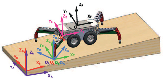
Figure 3.
Experimental platform.
- Frame {A}: this is the fixed frame of the system. Its z-axis is parallel to the gravity force but in the opposite direction. This frame will be considered as the reference frame. The origin of this coordinate axis is on the point of support of the right back leg at the beginning of the stabilization process.
- Frame : this is a fixed frame of the surface on which the system will be located. Its z-axis is perpendicular to this surface and the origin of this coordinate axis is on the point of support of the right back leg. The orientation of this frame with respect to {A} is []. The origin of this coordinate axis is on the point of support of each leg at the begining of the stabilization process. It is assumed that this frame is constant during the stabilization process. The origin of this coordinate axis is on the same point of the origin of frame {A}.
- Frame : this is an inertial frame related to the upper part of the base of the truck. Its z-axis is perpendicular to the upper part of the base of the truck. The origin of this coordinate axis is on the point of support of each leg. The orientation of this frame with respect to {A} is []. It is interesting to express the orientation of this frame with respect to {A} because the inclination measurements of the sensor that will be used in the control process are related to frame {A}. We shall define one frame for each leg.
- Frame : this is an inertial frame whose z-axis is perpendicular to the upper part of the base of the truck. It is similar to frame {C} but rotates about by (configuration parameter of the system). The origin of this coordinate axis is on the point of support of the right back leg. The orientation of this frame with respect to {C} is [0 0 ]. We shall define one frame for each leg, where will be different for each leg and will depend on the parameter of the system (see Figure 1b).
- Frame : this is an inertial frame whose z-axis is perpendicular to the upper part of the base of the truck. It has the same orientation to frame {C}. The origin of this coordinate frame is on the point that joins each leg to the base of the truck. We shall define one frame for each leg.
- Frame {F}: this is an inertial frame whose z-axis is perpendicular to the upper part of the base of the truck. It has the same orientation to frame {C}. The origin of this coordinate frame is in the geometric center of the base of the truck.
The inputs of the system are the positions of the linear actuators. When the length of the linear actuators is modified, the posture and the orientation of the system consequently change. The first step is to obtain the relation between the support point of the leg () and the point that joins the leg to the base of the truck (). We assume that the four legs are completely equal. Figure 4 shows a scheme of one leg. We represent the kinematic configuration of the four-bar leg by the location of its toe with respect to its clamp part with the base of the truck, whose vector depends on the features of the system and the position of the linear actuators. The coordinate frame of the leg is frame . is the translation between the origin of frame and frame expressed in the coordinates of frame .
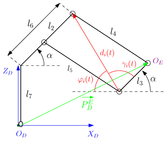
Figure 4.
Scheme of the mechanism of the leg.
In Figure 4, , , , , and are parameters of the system (see Table 1) and they are constant. However, and depend on the length of the linear actuator, .
The use of the cosine theorem makes it possible to obtain the relation between the angles and and the position of the linear actuator :
The translation between the origin of frame and frame , expressed in the coordinates of frame and taking into account that and , can, therefore, be expressed as:
Once the kinematics of one leg has been defined, the next task is to define the frames , and of the four legs. Figure 5a shows the definition of the frames for each leg. As will be noted in this figure, the orientation of the frames and is the same for the four legs and they are located on the support point of each leg and on the point that joins each leg to the base of the truck, respectively. However, the orientation of the frames are different for each leg and they are located on the support point of each leg.
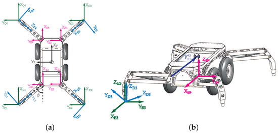
Figure 5.
(a) top view of the platform; (b) front view of the platform.
The translation vectors between the frames , corresponding to each leg i, and the frame {F}, which is located in the geometric center of the base of the truck (see Figure 5b), expressed in the coordinates of the frames , are constant vectors denoted , whose components are given in Table 2 and upper T means matrix transpose.
Table 2.
Values.
Keeping in mind that the system does not rotate about the axis (), the rotation that relates frame to frame {A} is . The same occurs with the rotation () that relates to frame {A} which can be expressed as where and were defined previously as the first two components of the orientation of the frame related to the upper part of the base of the truck ([]) with respect to the fixed frame of the system. This orientation varies depending on the configuration of the legs and the orientation of the surface on which the system is located, whereas and are the two first components of the orientation of the frame related to the surface on which the system is located ([]). Note that the frames have been defined in such a way that the third component of the orientations of the aforementioned frames is equal to zero ().
Upon observing Figure 5a, it will be noted that the rotation that relates frame to is different for each leg. These rotations, therefore, can be expressed as where i is the number of the leg, and this value can be defined as:
It is now possible to define the transformation that relates frame {A} to frame {F} as:
Upon simplifying and keeping in mind that =0, (see Equation (4)), we obtain that:
Equation (5) can thus be simplified to , where the transformation matrix is composed of the rotation and the translation vector from frame {A} to frame , for each leg. Moreover, since the orientations of frames {F} and are equal, the transformation matrix is just a translation of value .
Note that applying equation to the three legs that are in contact with the ground yields two nonlinear matrix independent equations. The problem of using this method is that the position of the support point of the legs varies throughout the stabilization process and these variations are unknown. Variables will, therefore, change throughout the stabilization process and they are uncertain. As a result, it is impossible to attain with this method a precise kinematic model that relates the position of the linear actuators to the orientation of the base of the truck without knowing this slipping.
3.1. The Problem of the Slipping of the System
The support point of the legs has a little displacement around the plane of the ground owing to the configuration of the four-bar mechanism used to move the legs of the system. Figure 6 depicts the relative movement of the support point and (blue line) when the extension of the linear actuators varies considering that the point is fixed thorough the movement (actually, is not fixed, but we do it in order to illustrate the relative movement between and ). Notice that this movement is not only vertical; the support point also follows a semicircular path. The configuration of the legs will, therefore, cause movements of the support point, , in the direction x of the frames . This phenomenon was observed with the real prototype, and as the absolute displacement of and depends on the configuration of the system, we only know the relative displacement between these two points.
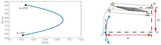
Figure 6.
Relative movement of the support point and .
It is important to highlight that the slipping is prompted for the configuration of the mechanism of the legs. The four-bar mechanism can change the height of the point , which is called displacement . However, unavoidably, a small displacement is produced which introduces some uncertainty in the position of in the plane of the ground (Figure 6a shows that is much smaller than ). Small wheels were located in the lower part of the system (see Figure 7a) in order to minimize the effort of the linear actuator at the time of executing the movement and surpassing the friction between the support point and the ground. The wheels of the legs were located in the plane of the four-bar mechanism in order to permit the rolling only in that plane. This configuration has two important features: (a) it allows smooth displacements of of each leg in the plane of the ground () because the wheels can roll in the plane of the leg minimizing the effort of the linear actuators and (b) the wheels of the four legs are in opposing directions because of the configuration of the system, thus avoiding the slipping of the whole system (see Figure 7b). It means that, if the linear actuators are braked, no slipping should appear in the system.
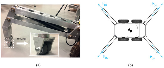
Figure 7.
(a) wheels of the system; (b) opposing movement of the wheels.
3.2. New Kinematic Model
One alternative by which to solve the aforementioned problem could be to use a sensor that measures the position of the support points of the legs. However, in this work, we propose a new alternative that allows us to obtain a kinematic model without having to use more sensors. Note that there is a component of the position of the support point of the legs that will be constant throughout the process of stabilization and is, fortunately, equal for the legs that are in contact with the ground (3 at least). This component is the component Z of the position of the support points expressed in the frame {B}. This allows us to reformulate the previous methodology in order to obtain the kinematic model of the system without having to use more sensors. Bearing this in mind, and defining a frame and for each leg with the same orientation as {B} and {A} but with the origin in each leg, we shall, therefore, define the kinematic model of the system as , in which is the j-row, k-column element of matrix . Elements are, therefore, equal for the three legs that are in contact with the ground and they do not depend on the sliding of the support points of the legs (these legs will be denoted by the superscript , and ). We consequently have two nonlinear independent equations and two unknowns (, ) when using this methodology. These equations are:
The accelerometer measures the orientations with respect to the fixed reference frame {A}, signifying that the transformation is not directly known. However, we can calculate it as where . The translation vector between and will be , in which because the support points of the legs slide around the plane of the ground, and the movement of the support points is therefore zero in the perpendicular direction of the ground. This allows us to obtain a kinematic model which has two equations and two unknowns and this is made possible by presenting the model in this different form.
can be simplified as follows:
where the first three components in the last column are the translation vector between the frames and {F} expressed in the frame , which is defined as . The last column of the transformation matrix between the frames and is .
Transformation can, therefore, be defined using (8) and (whose last column has been defined above and its rotation matrix is ) and the fact that , which is constant for the legs that are in contact with the ground, can be defined as:
where , and
Note that the expression above, which facilitates attaining the kinematic model, can be obtained because . This is possible because we present the model in a different and innovative manner.
We, therefore, define , and for the three legs that are making contact with the ground. The final three equations that define the kinematic model are:
where , and . The variable h is the component Z in the centre of the frame {B}, which is the perpendicular distance between this point and the ground.
The proposed kinematic model has three equations and six variables (, , , , and h). Knowing the extension of the linear actuators (, , ), this model makes it possible to obtain the orientation and the posture of the system (, and h).
3.3. Kinematic Model Validation
The purpose of this section is to validate the efficiency and the accuracy of the kinematic model proposed in this work by means of a software program and using the real prototype.
3.3.1. Simulation Results
Figure 8 and Figure 9 show the results obtained doing co-simulations with Matlab/Simulink and MSC ADAMS software and the results obtained using the proposed kinematic model (the orientation is obtained solving the Equations (10) and (11) using the parameters of Table 1, the orientation of the ground and the positions of the actuators and the height of the centre of frame {F} are obtained using (12)). This software has been used to simulate the kinematics of the system combining different positions of the linear actuator in order to asses the accuracy of the proposed kinematic model. During simulations, the system was placed on an inclined plane and a combined movement of the linear actuator was proposed. The plane on which the system is located has an orientation of and . In the initial configuration of the system, its four legs are touching the ground and the base of the system has an orientation of and . A trajectory that modifies the inclination in both directions is generated using the linear actuators in order to validate the kinematic model. The system was located in an inclined plane in order to demonstrate that the proposed kinematic model is valid for any inclination of the ground. Figure 8 shows the height of the center of frame {F} and Figure 9a,b show the pitch and roll angles of the system, respectively
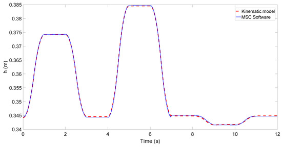
Figure 8.
Validation of the height of the centre of frame {F}.
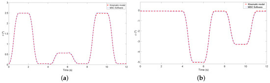
Figure 9.
(a) validation of the pitch angle (); (b) validation of the roll angle ().
The maximum errors of the orientation in the co-simulation are mm, and .
3.3.2. Experimental Results
Figure 10 and Figure 11 show the results obtained with the real prototype and the results obtained using the proposed kinematic model. A camera-based optical tracking system was used as an external sensor to validate the experimental results. This sensor consists of three infrared cameras that measure the orientation and posture of the system with very high precision. Appendix B describes how the inclination and the height of the centre of frame {F} are calculated in experimentation. The results obtained using the real prototype are compared with the inclination and height of the centre of frame {F} obtained using the proposed kinematic model, in order to validate its accuracy in the real prototype. The orientation is obtained solving Equations (10) and (11), using the parameters of Table 1, the orientation of the ground (which is known in the experiment) and the positions of the actuators, which are measured with the encoders of the linear actuators. The height of the centre of frame {F} is obtained using Equation (12).
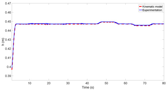
Figure 10.
Validation of the height of the centre of frame {F}.
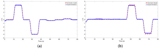
Figure 11.
(a) validation of the pitch angle (); (b) validation of the roll angle ().
In this case, the plane on which the system is located has an orientation of and . Figure 10 shows the height of the center of frame {F} and Figure 11a,b shows the pitch and roll angles of the system, respectively.
The maximum errors of the kinematic model concern the height of the system, mm, and the two components of the orientation and .
4. Workspace of the Robot
The whole system is a mobile manipulator principally composed of the mobile platform described in Section 2 and a very slender manipulator made of composite material with a length of m and a total mass of Kg. The purpose of this section is to obtain the workspace of the whole system.
The workspace of the system will be defined by the possible positions of the tip of the lightweight manipulator, which is above the truck. The workspace of the position of the tip of the lightweight, expressed in coordinates of frame {B} which has the origin on the support point of the right back leg, depends on the parameters of the system and the extension of the linear actuators, which has a range of extension between the extension needed to touch the ground with the leg and the maximum extension of the device [0.390–0.420]. The workspace is obtained using the kinematic model of the system to calculate the position of the center of frame {F} and adding the distance between the center of frame {F} and the tip of the manipulator and supposing that the system is in a flat ground ( and ). Note that the distance between the center of frame {F} and the base of the manipulator is m and the length of manipulator is described by m (see Figure 12a). The different positions of the tip can be obtained with the following equation and for all the combinations that assure that the extension of the four linear actuators are in the range [0.390–0.420]:
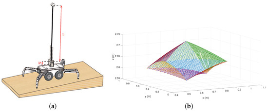
Figure 12.
(a) the whole system; (b) the workspace of the system.
Figure 12 shows that the shape of the workspace of the system is an object with eight curves’ faces. The workspace can, therefore, be approximated by using eight equations that define the curves’ planes of the eight faces. The conditions for the workspace of our robots are the following:
- ,
- ,
- ,
- ,
- ,
- ,
- ,
- ,
being [, , ] = [0.736,0.567,0.386]. These conditions define a workspace which is inside the real workspace and represent more than of the total workspace. This means that the robot can achieve the target if the points fulfill the previous conditions and less than 3% of the points are not included in the approximated workspace.
In the cases where the system is placed on an inclined plane ( or ), the workspace will be defined by the previous workspace (obtained for the case of flat ground) being rotated by . Therefore, to know if a specified point expressed in the frame {A} (fixed frame of the system) and respect the point of support of the right back leg and having an orientation of the ground and can be achieved for the system, we transform the coordinates of the specified point expressed in the frame {A}, , as follows:
Therefore, if the point [x,y,z] fulfills the previous eight conditions, it means that the system can achieve the target.
5. Design of the Controllers of the Linear Actuators
In our control scheme, we feed back the measurements of the linear actuator encoders. The control strategy consists of an inverse kinematics of the system described with a unified Jacobian model that is valid for all the configurations of the system. This control strategy is combined with linear actuator position controllers to make the dynamics between the linear actuator extensions and their references negligible and robust to motor frictions and parameters’ changes. The idea is to make use of the kinematic model described in the previous section to determine the linear actuator extensions through the inverse kinematics of the system that provide a precise control of the posture and the orientation of the system. The linear actuators extensions are simultaneously controlled by (proportional-integral) controllers.
5.1. Linear Actuators’ Dynamics
The dynamic model of a typical DC motor is a very well known second-order equation. As was explained previously, a linear actuator is a device that converts the rotational movement of a DC motor into linear movements. The equation that describes the dynamics of a linear actuator can, therefore, be expressed as:
where is the motor torque that is assumed to be proportional to the control voltage signal V, is the constant that relates the motor torques with the control voltages, and are the equivalent inertia and the viscous friction of the system, is the Coulomb friction of the motor and x is the linear position of the system. The transfer function of the system when considering the Coulomb Friction as a disturbance that will be canceled for the controller can, therefore, be expressed as:
5.2. Identification of the System
The identification process of the dynamics of the linear actuators was carried out for two different cases: (a) when the leg is not in contact with the ground and the system does not, therefore, have to move a load and (b) when the system is in contact with the ground and the load on the mobile platform (the total mass of the system is 50 Kg) is distributed over the four legs. In each case, ten steps with different amplitudes were used as input to the system. In Figure 13a,b, the applied voltage of the system and the extension of the linear actuator are shown, respectively, for case (a). In Figure 14a,b, the applied voltage of the system and the position of the linear actuator are shown, respectively, for case (b). These figures show that the response of the system to the steps are ramps with different slopes. It is, therefore, possible to conclude that the transfer function that relates the control signal (V) and the linear position of the actuator (x) can, for both cases, be approximated using the expression:
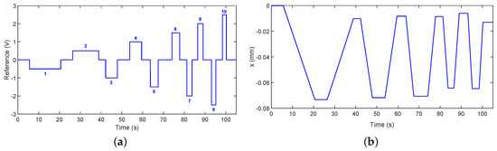
Figure 13.
(a) applied voltage in case (a); (b) extension of the linear actuator in case (a).
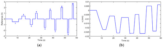
Figure 14.
(a) applied voltage in case (b); (b) extension of the linear actuator in case (b).
Note that Equation (16) tends toward Equation (17) if is much higher than 1. Figure 15a shows the relation between the control signal and the velocity of the system in both cases. Figure 15b depicts the constant K of the transfer function (17) for each step and for both experiments.
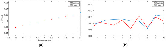
Figure 15.
(a) relation between the control signal and the velocity; (b) estimation of the parameter K of the transfer function (17).
The results show that the system behaves in a similar manner, regardless of whether or not it is carrying a load. This phenomenon occurs because the linear actuator has a very high reduction gear and the additional torque required to move a load, therefore, has very little influence on the dynamics of the system. Finally, a nominal value of with a maximum variation of was obtained in both experiments. This value is the mean of K in the ten steps of both experiments. The same study was carried out for the other three legs, obtaining similar results. It was, therefore, considered that the dynamics of the four legs of the system can be described using the following transfer function:
5.3. Design of the Controllers
In our control system, we feed back measurements of the linear actuator positions x. Figure 16 shows the control scheme of the linear actuators.
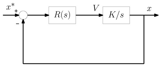
Figure 16.
Control scheme.
We propose a controller of the form:
Upon operating the characteristic polynomial (denominator of the closed-loop transfer function) of the system and equalizing to a second order transfer function, we obtain:
where p is the absolute value of the position of the poles of the closed-loop transfer function. Equation (21), therefore, enables us to obtain two parameters and two equations.
controllers of the form (19) were chosen because we need two parameters to ensure good trajectory tracking, providing precise and fast motor positioning responses and, above all, because their integral action eliminates the error in the steady-state that produces unmodelled disturbances such as Coulomb friction, .
6. Truck Height and Orientation Control System
The proposed control strategy combines the previous linear actuator position controllers with a unified Jacobian model, which is valid for all the configurations of the system, obtained from the inverse kinematic model developed in Section 3. The linear actuator extensions are calculated by using the inverse kinematics of the system. This provides a precise control of the posture and the orientation of the mobile platform. The linear actuator extensions are simultaneously controlled by the decentralized controllers of Subsection 5.3. These controllers have been tuned with high gains in order to make the closed loop dynamics of the linear actuators negligible (transfer functions between the actuator extensions and their references approximately equal to 1) as well as robust to motor frictions and parameters changes.
6.1. Inverse Dynamics
In this section, a new control strategy is proposed to control the orientation of the system (, ) and the height of the center of mass of the truck (h). The system has therefore three outputs and three inputs must be used in order to control them, which are the positions of three linear actuators . Assuming that the legs with these subindexes , and (see Figure 17) are in contact with the ground, three independent nonlinear equations are defined that can be expressed in a compact form as follows. Let us express Equations (10)–(12) in a matricial form as
where , and were defined in Section 3.2 and:
being the , and variables related to the three inputs through expressions (4).
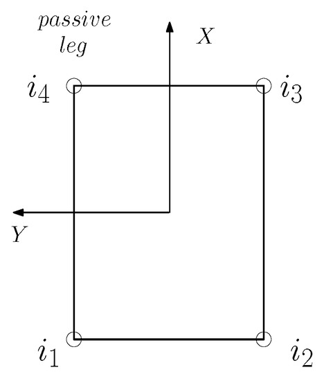
Figure 17.
Subindexes of the legs.
Then, is a vector function . Let us denote the Jacobian matrix of with respect to the output vector and the Jacobian matrix of with respect to the input vector . Differentiating Equation (22) with respect to time, it is obtained that
and the differential relationship between the derivative of the reference of the controlled variables and the desired derivative of the linear actuator extensions can be expressed in the following matricial formulation (see Appendix A for the values of the components of the matrices):
Note that the inversion of matrix in Equation (26) is very simple owing to the fact that
and
where
6.2. Obtaining Orientation of the Ground
The proposed control strategy uses the inversion of the kinematic model in order to calculate the trajectories of three linear actuators to control the three outputs of the system (, and h), provided that the orientation of the ground ( and ) is known. The first step in order to be able to use the control strategy of this work is, therefore, to calculate the orientation of the ground. This is done using the measurements of the inertial sensor (see Figure 2) and the extensions of the linear actuators when the system works in the second configuration at the instant at which the legs are in contact with the ground, and Equations (10) and (11) of the kinematic model. We have two nonlinear equations with two unknowns ( and ) that can be solved using numerical methods such as the Newton–Raphson method because the parameters of the system, the orientation of the base of the truck ( and ) and the extension of the linear actuators are known.
6.3. New Strategy Proposed for the Additional Leg
As mentioned previously, the system has 3 DOF and four legs that can be actuated. Note that the kinematic control is defined using the extension of the linear actuators (, and ) of three legs, and the control of the system also uses only these three linear actuators. The passive leg will, therefore, be used to make the system more stable, thus avoiding imbalance. The strategy proposed in this work is to calculate the position of the linear actuator () in order to fulfill the condition that the support point of the passive leg is in contact with the ground:
which can be expressed as
Equation (31), therefore, makes it possible to calculate the position of the linear actuator of the passive leg at each moment according to the position of the extension of the linear actuators and the orientation. Finally, the general control strategy proposed in this work is depicted in Figure 18.
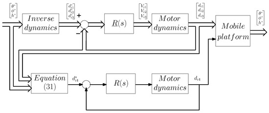
Figure 18.
Control scheme.
6.4. Experimental Results
This section shows some of the experimental results obtained after using the proposed control system when the system is in contact with the ground in order to demonstrate its efficiency. Figure 19 shows a photograph of the prototype.
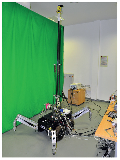
Figure 19.
Experimental platform.
Figure 20 and Figure 21 show the results obtained after using the control proposed in this work. It is possible to obtain a very good tracking of the three variables that we wish to control (, and h). A camera-based optical tracking system was used as an external sensor. A small error owing to the uncertainties in the kinematic model will also be noted. Figure 22a shows the extension of the actuators required to carry out the desired tracking of the posture and orientation of the system. The poles of the controller of the linear actuators were located in for the four linear actuators, and the following controller for the four linear actuators was obtained from Equation (21):
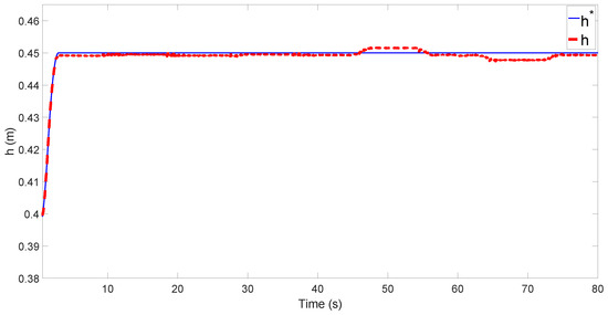
Figure 20.
Height of the center of mass of frame using the proposed control system.

Figure 21.
(a) using the proposed control system; (b) using the proposed control system.
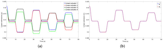
Figure 22.
(a) extension of the linear actuators; (b) extension of a linear actuator using Equation (32).
Finally, Figure 22b shows that an almost perfect tracking of the extension of a linear actuator is achieved using the controller (32).
The maximum errors of the system between the references and the outputs are mm, and .
7. Discussion
The new kinematic model has been tested by means of realistic co-simulation with Matlab/Simulink and MSC ADAMS software and with the real prototype. The results of the kinematic model have been tested by using software and placing the system on an inclined plane in order to test the kinematic model being validated when the system is on inclined ground. The co-simulations show that the model described the kinematics of the system quite well with an almost negligible error (maximum errors of mm, and ). These little errors are caused because the kinematic model assumes that the support point of the legs is at specific points, but the hypothesis is not perfectly true. This point will change slightly depending on the orientation of the system because the lower part of the leg is a surface. However, this error may be negligible.
In addition, the kinematic model has been tested using the real prototype. The experimental results show the good accuracy of the kinematic model. However, few errors appear in the model, particularly as regards the orientation (maximum errors of mm, and ). The maximum errors in experimentation are considerably greater than in simulations because the parameters of the system are not perfectly equal in the four legs owing to inaccuracies at the time of manufacturing the pieces.
The results of the identification of the dynamics of the linear actuators demonstrate that the system has similar behaviors if the system works with and without load. Therefore, the dynamics of the linear actuators can be approximated by the transfer function (18).
The control scheme shows a very good tracking of the output of the system ( mm, and ) using the control strategy proposed in this work. As can be seen from the results, the errors are similar to the errors obtained when validating the kinematic model. The next step of this work will, therefore, be to add an external loop that will feedback the measurements of the inertial sensor in order to correct the errors caused by inaccuracies in the parameters of the system. In addition to this, the results show the perfect trajectory tracking of the extension of the linear actuators. These results demonstrate that the hypothesis of approximating the dynamics of the linear actuators by the transfer function (18), for any configuration is valid because the load of the system has a negligible effect in the dynamics of the actuators. Finally, the workspace of the system considering the manipulator as a rigid one has been calculated. The obtained volume has been approximated using eight equations which represent 97% of the real workspace.
As was mentioned in Section 3.1, the wheels of the four legs are in opposing directions in order to avoid the slipping of the whole system. However, if the mobile manipulator placed above the mobile platform moves fast enough, it is possible that the reaction forces in the platform become bigger than the friction forces of the support points of the legs. Then, some slipping could appear in the mobile platform. For that reason, a simulation study of fast trajectories of the lightweight manipulator has been carried out in order to study this phenomenon. Anyway, the interaction between the manipulator and the mobile platform will be addressed in future works. For that reason, this phenomenon only is studied with some simulations. Figure 23 shows the results of co-simulations with Matlab/Simulink and MSC ADAMS software in order to compare the slipping that appears in the cases: (1) the linear actuators of the system are moving while the lightweight manipulator is stopped and (2) the lightweight manipulator is carrying out a fast trajectory ( in 1 s) while the linear actuators are braked. The initial position of the flexible manipulator is perpendicular to the plane of the mobile platform. During the first part of the movement, the linear actuators are moving in order to increase the height of the center of mass of the mobile platform, h, while keeping constant the orientation of the system ( and ). During the second part of the movement, the linear actuators are braked and the manipulator carries out a fast trajectory. In the upper part of Figure 23a, the trajectory of the height of the system, h, is shown, whereas, in the lower part of Figure 23a, the angular movement of the lightweight manipulator is shown. In Figure 23b, the module of the displacement of the support points of the legs in the plane of the ground, , is shown for each linear actuator. In that simulation, real parameters of the system have been used. The total mass of the mobile platform is approximately 50 Kg, whereas the mass of the lightweight manipulator with the camera at the tip is 1 Kg. The results show that the slipping that appears when the manipulator is moving is negligible (lower than 0.01 mm in each leg) because the configuration of the four legs does not allow it if the linear actuators are stopped. However, when the linear actuators are moving, the effect of the slipping is noticeable (around 3 mm in each leg). Notice that the weight of the manipulator is much lower than the weight of the mobile base. This is another advantage of using lightweight manipulators in mobile platforms: the reaction forces due to fast movements of the manipulator will have little influence in bulky platforms. Our mobile platform is not very big, but it has the possibility to extend its legs in order to increase the polygon support of the system and improve considerably the physical stability of the system. The interaction between the manipulator and the base platform has been only addressed analyzing the slippage caused by a fast movement of the manipulator. Only simulated results have been provided because it is not easy to precisely measure the produced small slippage. We have not noticed any vibrations caused by the possible manipulator-non rigid platform interaction, as the experimental measures given by the external optical system show in Figure 20 and Figure 21. Then, we can state that our platform is quite rigid.
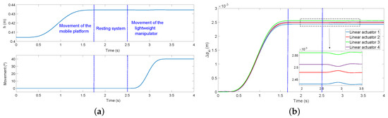
Figure 23.
(a) top view of the platform; (b) front view of the platform.
8. Conclusions
We have presented a new mobile platform with which to transport lightweight manipulators. Its main features are that the system has legs and wheels in order to carry out three different tasks: (a) transport the manipulator from one place to another, (b) increase the stability of the system, since it is able to position the base of the platform in a specific posture and orientation and the legs increment the area of the stability polygon and (c) legs help in the positioning of the tip of the manipulator. In this work, a new kinematic model is proposed which describes the kinematics of the system quite well and it is able to deal with the slipping problem of the support points of the legs. The kinematic model has been validated by means of a software program and using the real prototype, for both the cases that the system is located in an inclined plane and in a flat plane.
The proposed control strategy combines actuator control loops that feed back measurements of the linear actuator encoders with a feedforward controller based on the inversion of the kinematics of the system, this last term being in charge of the control of the posture and inclination of the system. Our experiments show that this inclination and posture open-loop control gives an accurate enough positioning for many applications.
It has also been verified that the configuration of the system does not affect the dynamics of the linear actuators because they have a very high reduction gear. Therefore, simple controllers have been proposed to design the actuators’ control loops.
Although the experimental results show the efficiency of the control scheme, there is still room to increase the accuracy in the positioning of our system as well as its robustness to small parametric uncertainties. Then, our next step will be to close an outer second control loop (around the already implemented inner actuator control loop) that feeds back the measurements of the inertial sensor in order to eliminate residual positioning errors (this sensor has only been used in this work to estimate the inclination of the ground).
Moreover, the system has a motor in the base of the truck (see Figure 19), which has not been included in this work. This additional joint will increase the workspace of the system. The study of the system with this additional joint will be the objective of future works.
Finally, the workspace of the system is defined considering the manipulator as a rigid one. Future works will consider the flexibility of this system in order to be more precise in the definition of the workspace for the lightweight manipulator of the real prototype.
Author Contributions
D.F.-T. and A.S.-M. developed the hardware and software of the device. V.F.-B. and D.F.-T. developed the kinematic model and the control system. D.F.-T. performed the experiments. D.F.-T., V.F.-B. and A.S.-M. wrote the paper.
Acknowledgments
This work has, in part, been supported by the Spanish Agencia Estatal de Investigación (AEI) under Project DPI2016-80547-R (Ministerio de Economía y Competitividad), in part by the European Social Fund (FEDER, EU) and in part by the Spanish scholarship FPU14/02256 of the FPUProgram of the Ministerio de Educacion, Cultura y Deporte.
Conflicts of Interest
The authors declare no conflict of interest. The founding sponsors played no role in the design of the study; in the collection, analyses or interpretation of data; in the writing of the manuscript; or in the decision to publish the results.
Appendix A
Appendix B
The camera-based optical tracking system, composed of three infrared cameras, was used to measure the height of the centre of frame and the inclination of the mobile platform. Therefore, the 3D positions of the four points depicted in Figure A1 were measured in order to know the height and the inclination of the prototype. The optical system measures the 3D positions with respect to the Frame . Therefore, using the 3D positions of , and , the inclination and can be easily calculated. After that, measuring the position of and the inclination of the ground, the height of the centre of frame can be easily obtained.
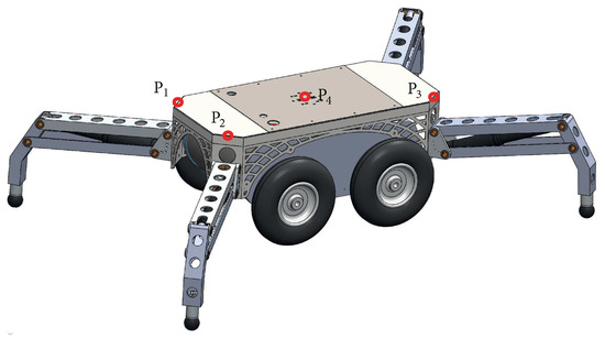
Figure A1.
Experimental platform.
This camera-based optical tracking system has a very high accuracy and it is able to measure the position of a specific point with a precision of mm. It was proved in experimentation that using the configuration of the measured points of the Figure A1 and this precision, the system is able to measure the inclination with a precision of .
References
- Dwivedy, S.K.; Eberhard, P. Dynamic analysis of flexible manipulators, a literature review. Mech. Mach. Theory 2006, 41, 749–777. [Google Scholar] [CrossRef]
- Benosman, M.; Le Vey, G. Control of flexible manipulators: A survey. Robotica 2004, 22, 533–545. [Google Scholar] [CrossRef]
- Kiang, C.T.; Spowage, A.; Yoong, C.K. Review of control and sensor system of flexible manipulator. J. Intell. Rob. Syst. 2015, 77, 187–213. [Google Scholar] [CrossRef]
- Bloch, A.; Baillieul, J.; Crouch, P.; Marsden, J.E.; Krishnaprasad, P.S.; Murray, R.; Zenkov, D. Nonholonomic Mechanics and Control; Springer: New York, NY, USA, 2003; Volume 24. [Google Scholar]
- Korayem, M.H.; Ghariblu, H. Analysis of wheeled mobile flexible manipulator dynamic motions with maximum load carrying capacities. Rob. Auton. Syst. 2004, 48, 63–76. [Google Scholar] [CrossRef]
- Korayem, M.; Shafei, A. A new approach for dynamic modeling of n-viscoelastic-link robotic manipulators mounted on a mobile base. Nonlinear Dyn. 2015, 79, 2767–2786. [Google Scholar] [CrossRef]
- Korayem, M.H.; Rahimi, H.; Nikoobin, A. Mathematical modeling and trajectory planning of mobile manipulators with flexible links and joints. Appl. Math. Model. 2012, 36, 3229–3244. [Google Scholar] [CrossRef]
- Freese, M.; Matsuzawa, T.; Oishi, Y.; Debenest, P.; Takita, K.; Fukushima, E.F.; Hirose, S. Robotics-assisted demining with gryphon. Adv. Rob. 2007, 21, 1763–1786. [Google Scholar] [CrossRef]
- Morelli, U.; Dalla Vedova, M.D.; Maggiore, P. Automatic Painting and Paint Removal System: A Preliminary Design for Aircraft Applications. In International Conference on Robotics in Alpe-Adria Danube Region; Springer: Cham, Switzerland, 2018; pp. 640–650. [Google Scholar]
- Glazunov, V.; Koliskor, A.S.; Krainev, A.; Model, B. Classification principles and analysis methods for parallel-structure spatial mechanisms. J. Mach. Manuf. Reliab. 1990, 1, 30–37. [Google Scholar]
- Chakarov, D.; Parushev, P. Synthesis of parallel manipulators with linear drive modules. Mech. Mach. Theory 1994, 29, 917–932. [Google Scholar] [CrossRef]
- Rao, A. Topological characteristics of linkage mechanisms with particular reference to platform-type robots. Mech. Mach. Theory 1995, 30, 33–42. [Google Scholar] [CrossRef]
- Stewart, D. A platform with six degrees of freedom: A new form of mechanical linkage which enables a platform to move simultaneously in all six degrees of freedom developed by elliott-automation. Aircraft Eng. Aerosp. Technol. 1966, 38, 30–35. [Google Scholar] [CrossRef]
- Gough, V. Universal tyre test machine. In Proceedings of the 9th International Technical Congress, London, UK, 2–6 May 1962. [Google Scholar]
- Lee, K.M.; Shah, D.K. Kinematic analysis of a three-degrees-of-freedom in-parallel actuated manipulator. IEEE J. Rob. Autom. 1988, 4, 354–360. [Google Scholar] [CrossRef]
- Russo, A.; Sinatra, R.; Xi, F. Static balancing of parallel robots. Mech. Mach. Theory 2005, 40, 191–202. [Google Scholar] [CrossRef]
- Ottaviano, E.; Ceccarelli, M.; Tavolieri, C. Kinematic and dynamic analyses of a pantograph-leg for a biped walking machine. In Climbing and Walking Robots; Springer: Berlin, Germany, 2005; pp. 561–568. [Google Scholar]
- Liang, C.; Ceccarelli, M.; Takeda, Y. Operation analysis of a one-DOF pantograph leg mechanisms. Proc. RAAD 2008, 8, 1–10. [Google Scholar]
- Fedorov, D.; Birglen, L. Design of a self-adaptive robotic leg using a triggered compliant element. IEEE Rob. Autom. Lett. 2017, 2, 1444–1451. [Google Scholar] [CrossRef]
- Morales, R.; Chocoteco, J.; Feliu, V.; Sira-Ramírez, H. Obstacle surpassing and posture control of a stair-climbing robotic mechanism. Control Eng. Pract. 2013, 21, 604–621. [Google Scholar] [CrossRef]
- Cambera, J.C.; Chocoteco, J.A.; Feliu-Batlle, V. Modeling and Identification of a Single Link Flexible Arm with a Passive Gravity Compensation Mechanism. In Proceedings of the 2018 IEEE International Conference on Robotics and Automation (ICRA), Brisbane, Australia, 21–25 May 2018; pp. 7704–7710. [Google Scholar]
- Joshi, S.A.; Tsai, L.W. The Kinematics of a Class of 3-dof, 4-legged Parallel Manipulators. J. Mech. Des. 2003, 125, 52–60. [Google Scholar] [CrossRef]
© 2018 by the authors. Licensee MDPI, Basel, Switzerland. This article is an open access article distributed under the terms and conditions of the Creative Commons Attribution (CC BY) license (http://creativecommons.org/licenses/by/4.0/).