Article

Game Theoretical Demand Response Management and Short-Term Load Forecasting by Knowledge Based Systems on the basis of Priority Index

1
Department of Computer Science, COMSATS University Islamabad, Islamabad 44000, Pakistan
2
Department of Electrical Engineering, COMSATS University Islamabad, Islamabad 44000, Pakistan
3
Department of Computer Science and Information Technology, Alhamd Islamic University, Islamabad 44000, Pakistan
4
Department of Computer Science, Islamic International University, Islamabad 44000, Pakistan
5
Department of Computer Science, Air University, Islamabad 44000, Pakistan
*
Author to whom correspondence should be addressed.
Electronics 2018, 7(12), 431; https://doi.org/10.3390/electronics7120431
Submission received: 15 November 2018 / Revised: 3 December 2018 / Accepted: 7 December 2018 / Published: 12 December 2018
(This article belongs to the Section Computer Science & Engineering)

Abstract

:
Demand Response Management (DRM) is considered one of the crucial aspects of the smart grid as it helps to lessen the production cost of electricity and utility bills. DRM becomes a fascinating research area when numerous utility companies are involved and their announced prices reflect consumer’s behavior. This paper discusses a Stackelberg game plan between consumers and utility companies for efficient energy management. For this purpose, analytical consequences (unique solution) for the Stackelberg equilibrium are derived. Besides this, this paper presents a distributed algorithm which converges for consumers and utilities. Moreover, different power consumption activities on the basis of time series are becoming a basic need for load prediction in smart grid. Load forecasting is taken as the significant concerns in the power systems and energy management with growing technology. The better precision of load forecasting minimizes the operational costs and enhances the scheduling of the power system. The literature has discussed different techniques for demand load forecasting like neural networks, fuzzy methods, Naïve Bayes, and regression based techniques. This paper presents a novel knowledge based system for short-term load forecasting. The algorithms of Affinity Propagation and Binary Firefly Algorithm are integrated in knowledge based system. Besides, the proposed system has minimum operational time as compared to other techniques used in the paper. Moreover, the precision of the proposed model is improved by a different priority index to select similar days. The similarity in climate and date proximity are considered all together in this index. Furthermore, the whole system is distributed in sub-systems (regions) to measure the consequences of temperature. Additionally, the predicted load of the entire system is evaluated by the combination of all predicted outcomes from all regions. The paper employs the proposed knowledge based system on real time data. The proposed scheme is compared with Deep Belief Network and Fuzzy Local Linear Model Tree in terms of accuracy and operational cost. In addition, the presented system outperforms other techniques used in the paper and also decreases the Mean Absolute Percentage Error (MAPE) on a yearly basis. Furthermore, the novel knowledge based system gives more efficient outcomes for demand load forecasting.

1. Introduction

In the modern day world, smart meters offer two way communication between the users and the utilities. This communication leads towards a prevalent computing environment, which develops large-scale data with high velocity and veracity [1]. The resultant data also give rise to a time series concept. This phenomenon generally includes power consumption measurements of appliances over a specific time interval [2]. The techniques of big data are proficient enough to utilize resultant huge volumes data of sequential time series. Moreover, these techniques also assist in data-driven decision making. Besides, this big data can update utilities to learn power consumption patterns of consumers, predicting demand and averting blackouts.
The utilities are keen on finding the optimal ways for cost reduction. Moreover, electricity companies desire to increase their yields by acquainting their consumers with effective programs like Demand Side Management (DSM) and demand response. Currently, marginal success has been observed in achievement of goals for these programs. However, viable results still need to be achieved [3]. Furthermore, implementation of DSM and demand response is a challenging task for utilities. It is difficult to comprehend and conclude the behavior of every individual consumer. Moreover, it is also challenging to customize strategies that include profit contrary to distress from varying behavior of consumers on the basis of energy-saving policies introduced by utilities. Besides, the association between consumer behavior and the constraints that affect power utilization patterns are non-static, i.e., the activities of consumers keep on changing from time to time [4].
Usually, the behavior of consumers is reliant on weather and seasons, which has a capricious effect on power utilization decisions. Thus, active participation of consumers in customized power management is crucial for energy saving schemes. The companies should give timely response on power consumption and associated costs [5]. Consequently, it is challenging to design such models that are proficient enough to evaluate energy time series from smart meters. Also, it is stimulating to train the model that predicts power consumption.
The aforementioned discussion helps to study the influence of consumers’ behavior on power consumption and to forecast the energy utilization patterns. This analysis can assist the utilities to develop power saving strategies. Moreover, the utilities can design programs to stabilize the demand and supply of energy ahead of time. For instance, short term forecast is related to daily and weekly power usage. This type of prediction is best suitable when there is a need to enhance scheduling and distribution. Alternatively, medium term forecasting is related to weekly and monthly forecasting. Besides, long term forecasting is about yearly predictions of energy consumption. Medium and long term predictions are capable of maintaining the equilibrium between the production of smart grid and strategic scheduling [6]. However, such a task is very challenging as it is significant to mine complex interdependencies between appliance usages where numerous data streams are taking place.
Generally, DRM can be characterized in two extents, which are the utilities and consumers. There has been substantial quantity of work done in power systems to maintain the balance between supply and demand [7]. However, these studies have laid emphasis on the financial aspects on the planning and production levels. Moreover, these studies are unable to take both consumer and utility as a substantial constituent. Contrariwise, the literature on consumer and utility has presented models to increase user comfort, devoid of taking the cost of power or the profits of the utilities [8]. This paper takes motivation from this phenomenon. Moreover, this paper observes the increased profits for consumers and utilities.
This paper analyzes the collaborations between several utilities and consumers. Both entities share mutual objectives, i.e., maximization of their payoffs. The utilities can increase their profits by setting a suitable price per unit. Nonetheless, the users select a specified amount of power to purchase from any utility on the basis of announced prices. Furthermore, the purchasing behavior of consumer is dependent on the prices settled by the company. Likewise, the behavior of utilities is reliant for the prices settled by other utilities. Thus, for solving these challenging collaborations between consumers and utilities, this paper employs a game theoretical framework. This paper presents a Stackelberg game plan between consumers and utilities. In this game, the utilities play a non-cooperative game and the users look for their best optimum response.
The systematic and proficient utilization of electrical power is a hot debate topic in today’s world [9]. The optimal power management and maintaining balance between demand and supply are considered as challenging tasks for modern power systems [10]. Moreover, the prediction of uncertain production of renewable energy resources [11] and short-term load forecasting [12] are measured as significant components of the power grid for optimal power scheduling. Besides, short-term load forecasting has wide applications in the energy market like load scheduling, unit commitment and power production [13]. It has been observed in the literature that error maximization in short-term load forecasting can result in substantial growth in the utility operating expenses. Thus, enhancing the accuracy of predicted results is a challenging task and vital issue in power management.
The proximity of choosing a similar day to the target day is very crucial for selecting the similar day along with temperature, according to previous studies. In this regard, this paper proposes a different priority indexing technique for selection of similar days by analyzing the date proximity and temperature similarity. Moreover, the date proximity used in this paper is the total number and nature of days between selected and similar days. In contrast, the historic power load data is categorized according to nature of days in demand prediction. Furthermore, this paper also presents four different day types and two data-sets are presented for utilization of historical power load data. In addition, the proposed knowledge based short-term load forecasting method employs monthly and weekly data for two different data-sets. The best optimum results for short-term load forecasting will be achieved by grouping of prediction results obtained from these two data-sets.
The consideration of exceptional temperature for any region is ineffectual because of variations in temperatures in a vast topographical zone. A vast topographical zone is separated into three climate types in [14]. Moreover, the temperature of three cities is labeled as cold, moderate, and warm. The biased integration of these temperatures is presented as the temperature of the huge region. The temperature is taken in [15] and the whole system is distributed in different regions. Besides, the short-term load has been forecasted by some regression techniques. However, the precedence of choosing similar days is also unnoticed in previous studies.
This paper divides the entire system in nine regions. Moreover, the climatic conditions of only one city is chosen from every region. The knowledge based short-term load forecasting is employed to every region after the consideration of temperature. In addition, the predicted power load of the entire system is the aggregate of predicted load of particular regions. The impact of temperature is believed to be much more efficient and result improving when the system is divided.
The proposed system model is employed in Pakistan’s National Power Network (PNPN), which is taken as a sample system in this paper. In the proposed system model, Affinity Propagation (AP) [16], and Binary Firefly Algorithm (BFFA) are used as hybrid model. The proposed system model shows a significant decrease in MAPE in comparison with other traditional knowledge based methods. This paper uses algorithms of Deep Belief Network (DBN) and Fuzzy Local Linear Model Tree (F-LOLIMOT) for comparison purposes. The experimental results specifies that the proposed model requires minimum time for computation when associated with DBN and F-LOLIMOT.
The major research contributions of this paper include the proposition of the priority index for selection of similar days by means of temperature of specified regions and date proximity. Moreover, the historic power load is separated in two different data-sets in the paper. Subsequently, the data-sets predict the short-term load and then the final outcome is supposed to be more precise. The final outcomes are achieved by the summation of predicted results from two data-sets. Furthermore, the paper makes the impact of temperature effective by dividing the system in different regions.
The remaining paper is organized in following manner: Section II presents the previous work done, Section III provides a brief discussion of a Stackelberg game and demonstrates the distinctiveness and existence of the Stackelberg Equilibrium. Moreover, Section IV discusses the categorization of knowledge based short-term load forecasting and Section V employs the proposed method on different topographical regions. Moreover, results and their discussion are presented in Section VI and Section VII concludes the paper.

2. Related Work

The challenges addressed in Section I are also discussed in the literature through methodologies of big-data. A brief discussion of behavioral power consumption data to acquire better energy competence are presented in [6]. Likewise, the influence of developmental fluctuations for energy savings was observed by [17]. The study also discussed the contribution of consumers to collaborate with the utilities and better energy savings were highlighted.
The literature has proposed many novel methods for short-term load forecasting like fuzzy [18], exponential smoothing [19], regression based [20], neural networks [21], and others. Moreover, every proposed model has incorporated some techniques. For example, regression based processes are usually comprised of Autoregressive Integrated Moving Average (ARIMA) [22], Auto-Regressive Moving Average (ARMA) [23], Support Vector Regression (SVR) [24], and Auto-Regressive Moving Average with Exogenous variable (ARMAX) [25]. Nevertheless, it is essential for aforementioned techniques to learn the process by bulks of preceding data for tuning of various parameters. Furthermore, the complexities of these techniques, minimum time of computation and memory essentials of knowledge based model, can initiate a different perspective to knowledge based short-term load forecasting.
In literature, there are some works cited in knowledge based systems that employ a similar day method [26,27,28]. Although, there is a lot of room for enhancement in this scenario which can be studied. The authors in [29] proposed a knowledge based system for short-term load demand forecasting. However, the paper overlooked the consequences of temperature. The change in temperature can cause fluctuations in the load demand. Consequently, the effect of temperature must be included in the short-term load forecasting. The different eight day categories are enumerated in [30].
Moreover, average stabilized loads of historic data for every day has been evaluated by means of least and maximum load per hour. Furthermore, the least and maximum load for 11 days was forecasted by means of regression techniques. The Mean Absolute Percentage Error (MAPE) of Irish electrical power system attained was 2.52%. Moreover, the temperature was also incorporated in this study and was associated with 3.86% by the statistical technique in [31].
The authors in [32] calculated the weighted mean load of every hour for three preceding and similar days for short-term load forecasting. Moreover, the impact of temperature on prediction of short-term load is also considered by means of exponential association between power demand and temperature. Likewise, the mean prediction error for a daily peak load of France was attained 2.74% in [32]. Besides, the consequences of temperature, wind pressure and humidity, was scrutinized in [33]. The MAPE calculated in this study was 1.43%. The study in [23] was almost equivalent to the proposed model presented in [22]. Moreover, the MAPE achieved in this study was between 1.23% to 3.35% in seven different states of America [34].
The mean prediction error for daily peak load in [24] was achieved 4.65% for weekdays and 7.08% for weekends of three different states of Turkey [35]. This mean prediction error was achieved after smoothing the temperature discrepancies throughout the day. The precedence of similar days is overlooked in previous studies. It is obvious that there are numerous days which are advantageous for the knowledge based forecasting of load. Nevertheless, the best suitable preference of these same days has a substantial effect on forecasting results.
The consequences of temperature are neglected in [36] in terms of priority index. Moreover, in [37] a priority index for medium term load prediction was presented. The proposed model was based on the similarity of temperature for the selected day. The mean error achieved in [37] for Western States of America was 3.25% for summer season. Besides, few values of error were attained that were more than 6%. Though, the temperature was the only parameter, which was assessed in this study and the proximity of chosen day to similar day was ignored. It is a well-known fact that same days do not have alike temperature. Moreover, the similar days must be near to the target days in order to avert the selection of similar days with similar temperature and different power load.
The work presented in [38] used the Bayesian network to forecast activities of different residents by a particular appliance. However, the model was not efficient enough to be functional towards real world circumstances. The authors in [39] and [40] discussed a multi-label and time sequence based classifier model for a decision tree taking appliance association as a correlation. The basic purpose of their model was to predict the power consumption of the appliance. Though, the authors merely observed the past 24 h frame for future forecasting.
The work in [41] presented the association rule mining method to classify the interdependence between power consumption and appliance usage to help power saving, anomaly detection, and demand response. Nevertheless, this work lacked the proper rule mining process and appliance-appliance association.
At present, Artificial Neural Network (ANN) and SVM are considered to work efficiently for non-linear time series sequences. Karatasou et al. [42] demonstrated the practical implementation of ANN in forecasting power expenditure of a building accompanied by statistical study. In [43,44], a model is presented which hybrids the Support Vector Regression (SVR) and Immune Algorithm (IA) to estimate local yearly report and power load in Taiwan.
Zhao et al. [45] presented a framework, which employed SVM to predict residential power utilization in the humid area. Moreover, the study took meteorological conditions of that particular area. Besides, Xuemei et al. [46] suggested Least Square Support Vector Machine (LS-SVM) for chilling load prediction [47] for a residential zone in Singapore. The forecasting was done by hourly weather information.
Wang et al. [48] discussed that the SVM based models have proven to be efficient as compared to ANN and ARIMA configurations. They employed Differential Evolution (DE) and SVM to predict the configurations for yearly energy consumption. Conversely, the development of SVM model is influenced by the category and constraints of the kernel function. Generally, it is discussed in literature that the tuning constraints of SVM is a challenging task [49]. In addition, a number of models are presented in literature to tune the parameters of SVM by techniques of machine learning and artificial intelligence.
Ogliari et al. [50] proposed a hybrid model using Neural Network and Genetical Swarm Optimization for energy prediction. The authors in [51] combined SVM with algorithms of Simulated Snnealing to predict yearly load. On the subject of optimization techniques, Jaya Algorithm has achieved attention in the last few years as a metaheuristic computing technique. The authors in [52] and [53] observed that Jaya Algorithm outperforms other optimization techniques. Moreover, Jaya Algorithm has also been employed for various real work applications.
There is a variety of literature available on the topic of game theory and DRM. In [54], the authors have discussed power utilization and forecasting as a non-cooperative game plan. This basic aim was to maximize the cost functions. Likewise, the authors in [55] have proposed a distributed set-up. In this set-up, the cost function is demonstrated by its dependence on inclusive load. The consumers adjusted their behavior for power consumption on the basis of cost function introduced by the utility. The authors in [56] presented a theoretical framework for mutual optimization of investment and functioning of a smart grid. Moreover, the aspects of power storing, renewable energy integration, and demand response were taken into consideration. The paper signified the sharing of portfolio decisions, day-ahead pricing, and scheduling. They also presented the benefits of integrated renewable energy and demand response in terms of minimizing the sharing cost.
A robust optimization has been discussed in [57] in order to increase the utility of the end-user by hourly prediction. The study presented in [58] laid emphasis on the knowledge and interest of users to be aware of the announced electricity prices. The study proposed a technique to cope with preferences of the consumers to increase power competence and consumer satisfaction. Moreover, a dynamic cost price has been introduced to motivate users for attaining a cumulative load [59]. Also, this load was handled by different utilities and DRM was scrutinized for bi-directional communication between consumers in the micro-grid. The authors in [60] and [61] discussed the dynamic pricing in detail for smart energy model of a smart grid. The discussed model was dependent on renewable energy sources, which were further integrated with intelligent control that processed information from a smart metering devices.
The studies discussed above are inadequate to meet the needs, i.e., the electricity firms considered utility companies as a single firm. This study differs in this context as this incorporates numerous utilities and consumers. Moreover, the basic aim of both entities is to increase their profits (remunerations) by game theoretic approach. Besides, there is a broad literature and findings available on the Stackelberg game on the topics of profits maximization, congestion control, and interactive communication [62,63].

3. Game Theoretical Problem Formulation

This study takes n consumers and UC utility companies in consideration. Besides, the energy sources of the utilities include non-renewable and renewable resources. In literature, it is observed that power generators, which are centered on the energy of fossils utilize a definite amount of energy. Moreover, the energy of fossils is also supposed to be harmful for the environment. Contrarily, renewable energy sources are considered environmentally friendly. However, renewable resources have inherent natural stochastic behavior, which makes it difficult to predict and control. The studies show that uncertainties are common with renewable resources. Furthermore, Markov chain (discrete time) has been extensively employed in literature for the generation of power from renewable resources [64].
This study takes residential type consumers into account. In addition, all users have dissimilar requirements for power consumption. The study also distinguishes the users based on their financial plans; i.e., purchasing power of electrical energy. Likewise, this study proposes a utility function for every consumer. The function shows an increment using the total expanse of power that any consumer is able to utilize. Moreover, this paper integrates cost parameters for every consumer.
The UC and n have established a two way communication using the advanced metering infrastructure for pricing swapping and information sharing. Conversely, UC can also communicate with one another. The n collect the value (cost) facts from the UC . In return, the UC then provide their services to n.
Power initiation, dissemination, and expenditure can be divided in three ways [65]: Power generators, UC , and n. This paper emphasizes the communication between n and UC . Moreover, this paper assumes that UC show a fluctuating behavior at the business level. Inspired from the game theory models, the UC can play a vital part in an economical marketplace. No participant is capable enough to affect the market price of electricity through his particular activities. Thus, the market price is such constraint over which UC have no control. Moreover, the UC need to increase their production up to the point where the minimal cost is equivalent to the cost of the market. This phenomenon occurs once the total contributors increase and no contributor is authorized to govern an enormous power generation quantity. Nonetheless, this study proposes a predetermined figure of UC (contributors). This scenario depicts that every utility will announce its own price according to its generation capacity. Table 1 shows the list of symbols used.

3.1. Analysis of User and Utility Company

The cost for every consumer shows fluctuation when there are various utility firms having diverse electricity costs. Moreover, the setting of cost is highly reliant on the rates of other UC . In this regard, game theory offers an ordinary pattern to represent the activities of n and UC . Consequently, the UC settle the cost for each unit of energy and then publicize this to consumers. The users then respond back to the cost by demanding an optimal amount of power from the UC . In this case, UC play first. The consumers then decide on the basis of announced prices. Moreover, both events are in sequence. The events are that the utilities play primarily and at that time the consumers decide their verdict based on the cost. Hence, this paper models the communication between the UC and n by a Stackelberg game [66]. The proposed game model takes the UC as influential (leaders) and users as followers. Moreover, the proposed model also considers the events as a multiple leaders and followers game.

3.1.1. Analysis of User Side

Assume that d n 0 , u c 0 is the request of consumer n 0 from a utility uc 0 . Hence, the value of a consumer n 0 , C c o n s , n 0 can be expressed as:
C c o n s , n 0 = γ n 0 uc 0 UC ln ( d n , u c 0 + τ d n 0 ) . uc 0 UC
Here γ n 0 and τ n 0 are constants. Also, the ln function is extensively employed in literature for user making decisions [67]. The valuable function used for consumer n 0 in Equation (1) is interrelated to the function γ n 0 ln d n 0 , u c 0 .
The consumer will recompense - when the valuable function γ n 0 ln d n 0 , u c 0 is used regarding u c 0 , such that, d n 0 , u c 0 = 0. When d n 0 , u c 0 and τ n 0 are equivalent to 0, then benefit of n 0 regarding uc 0 begin to be finite. Generally, the representative cost of τ n 0 = 1.
Suppose κ u c 0 is the per unit cost given by any utility company uc 0 and B n 0 0 is the total expenditure of any consumer n 0 . Each uc 0 has given a distinct price rates of electrical energy [ κ 0 , κ 1 ,……, κ c ] when n 0 n . Subsequently, the n 0 computes the best demand response through resolving best optimum solution ( OS c o n s ) given in Equation (2).
d n 0 = m a x ( d n 0 , u c 0 ) C c o n s , n 0 uc 0 UC ,
where uc 0 UC κ c d n 0 , u c 0 B n 0 ,
d n 0 , u c 0 0 uc 0 UC
OS c o n s is a convex optimization problem. Therefore, the obtained solution is distinctive and optimal.
This paper considers the scrutiny accompanied by UC consumers and three UC s. Thus, they seek for best optimum solution in this scenario for a specified uc 0 can be expressed as follows:
d n 0 = m a x ( d n 0 1 , d n 0 2 ) γ n 0 u c 0 = 1 3 ln ( d n + τ d n 0 , u c 0 ) ,
where κ c d n 0 , 1 + κ c d n 0 , 2 B n 0 and d n 0 , 1 + d n 0 , 2 0 .
The paper employs Lagrange multipliers ( Λ n 0 , 1 , Λ n 0 , 2 , Λ n 0 , 3 ) for the respective UC and setting of parameters as discussed above. Thus, the Equation (4) can be rewritten as:
υ c o n s , n 0 = γ n 0 u c 0 = 1 3 ln ( d n 1 + τ d n 0 , u c 0 ) Λ n 0 , 1 ( u c 0 = 1 3 κ c d n , u c 0 B 1 ) + Λ n 0 , 2 d n 0 , 1 + Λ n 0 , 3 d n 0 , 2 .
The values of the Lagrange multipliers are used as strategies for finding the local maximal and minimal of the function subjected to inequality constraint. Thus, it improves the performance of Equation (5).
Λ n 0 , 1 ( u c 0 = 1 3 κ c d n , u c 0 B n 0 ) = 0 .
Moreover, setting Λ n 0 , 2 d n 0 , 1 and Λ n 0 , 3 d n 0 , 1 generates Equation (6) to 0. Whereas, Λ n 0 , 1 > 0 , Λ n 0 , 2 , Λ n 0 , 3 , d n 0 , 1 , and d n 0 , 2 0 .
The first order optimality condition for linear, best optimum solution and maximization problem is by setting υ c o n s = 0 . Here, υ c o n s = ( υ c o n s n 0 n ). All of the n are interconnected by κ c . Also, υ c o n s = 0 shows that,
( υ c o n s , n 0 ) ( d n , u c 0 ) 1 = 0 n 0 n , uc 0 UC .
Also,
γ n 0 ( τ n 0 + d n 0 , 1 ) ( Λ n 0 , 1 τ 1 + Λ n 0 , 2 )
and
γ n 0 ( τ n 0 + d n 0 , 2 ) ( Λ n 0 , 2 τ 1 + Λ n 0 , 3 ) .
Next, this paper has considered four of the cases, which the n 0 can avail.

Case 1

If d n 0 , 1 and d n 0 , 2 are greater than 0, then Λ n 0 , 2 = Λ n 0 , 3 = 0 . So, Equations (8) and (9) are generalized as:
d n , u c 0 = γ n 0 ( τ n 0 κ u c 0 Λ n 0 , 1 ) ,
where n 0 n and u c 0 = 1 , 2 , , n . Now, using Equation (6) in Equation (10),
3 ( γ n 0 Λ n 0 , 1 ) 1 = B n 0 + τ n 0 uc 0 = 1 3 κ u c 0 .
Thus, Equation (11) becomes Equation (12) after simplification.
3 d n , u c 0 κ u c 0 = ( B n 0 + τ n 0 u c 0 = 1 3 κ u c 0 ) τ n 0
Here value of uc 0 varies; i.e., 1, 2, or 3.

Case 2

If d n 0 , 1 > 0 and d n 0 , 2 are equivalent to 0, then τ n 0 = ( B n 0 + τ n 0 u c 0 = 1 3 κ u c 0 ) / 3 κ u c 0 . As discussed above that Λ n 0 , 2 d n 0 , 1 corresponds to 0. This paper derives Equation (13) by considering the cost of the first utility.
d n 0 , 1 = γ n 0 τ n 0 Λ n 0 , 1 κ 1 .
This paper further expands Equation (6) to include extra parameter and ease simplification. Thus, Equation (14) is derived.
Λ n 0 , 1 ( γ n 0 κ 1 Λ n 0 , 1 τ n 0 B n 0 ) = 0 .
As Λ n 0 , 1 > 0 and γ n 0 κ 1 Λ n 0 , 1 τ n 0 B n 0 = 0 , which refers to the point that Λ n 0 , 1 = γ n 0 / ( κ 1 τ n 0 + B n 0 ) . Now, evaluating this in Equation (13),
d n 0 , 1 = κ 1 τ n 0 + B n 0 τ n 0 κ 1 .
Equation (15) is now equivalent to B n 0 / κ 1 . Moreover, Equation (15) can also be presented as:
d n 0 , 1 = τ n 0 ( κ 1 + κ 2 ) + B n 0 3 κ 1 τ n 0 ,
where d n 0 , 1 = ( ( τ n 0 ( κ 1 + κ 2 ) + B n 0 ) / 3 κ 1 ) + ( ( τ n 0 ( κ 1 + κ 2 ) B n 0 ) / 3 κ 1 ) .

Case 3

If d n 0 , 1 is equivalent to 0 and d n 0 , 2 > 0 , then the identical scrutiny can be valuated as specified in Case 2. This paper considered the cost of the second utility; thus, the demand of users with respect to the second utility is given in Equation (17).
d n 0 , 2 = τ n 0 ( κ 1 + κ 2 ) + B n 0 3 κ 2 τ n 0 .
Subsequently, Equation (17) is now equivalent to B n 0 / κ 2 .

Case 4

If d n 0 , 1 and d n 0 , 2 both are equivalent to 0, then Λ n 0 , 1 , Λ n 0 , 2 , and Λ n 0 , 3 are real and positive values. It is noted that Case 4 is assumed as best case which rarely occurs only when κ u c 0 = or else B n 0 0 .
This paper has satisfied the power and cost parameters as equalities in Case 1, 2, and 3. However, this scenario cannot be mapped on Case 4. This study further assumes that there are n consumers in total and UC utilities that satisfies the equality conditions in previous cases for a given set of κ u c 0 . So, Equations (12), (16), and (17) can be combined in the above discussed scenario as:
d n 0 , u c 0 = τ n 0 uc 0 UC κ u c 0 + B n 0 κ u c 0 UC τ n 0 .
In Equation (18), d n 0 , u c 0 0 , n 0 n and u c 0 UC . As d n 0 , u c 0 0 . So,
τ n 0 ( uc 0 UC κ ϱ ) + B n 0 > τ n 0 κ u c 0 ( UC 1 ) .

3.1.2. Analysis of Utility Companies

This study assumes that E u c 0 ( UC uc 0 ) depicts the available electrical energy of UC . The aim of every UC is to vend the energy to gain maximum profit. For instance, if there is only one UC then this firm will settle the price range according to its ease as there is no competition involved. However, this study takes two basic strategies that decide the cost range of any UC . Firstly, it can be the economical conditions of average consumers and secondly, it could be an aspect of competitiveness among UC s . Furthermore, the UC s also take part in choosing the best optimum cost (game) with another. Additionally, this study expresses the maximum profit E p r o d , u c 0 of any UC as:
E p r o d , u c 0 ( κ u c 0 , ξ u c 0 + 1 ) = κ u c 0 n 0 n d n 0 , u c 0 .
Here, ξ u c 0 + 1 is cost of UC apart from uc 0 . Thus, the best optimum solution for any UC can be related in terms of OP p r o d and can be expressed as:
ξ = m a x ( κ u c 0 ) p r o d , u c 0 E ( κ u c 0 , ξ u c 0 + 1 ) , u c 0 UC
where n n 0 d n 0 , u c 0 E u c 0 and κ u c 0 > 0 , UC u c 0 . The maximum profit of any UC is fluctuating in relation to energy for a constant κ u c 0 . According to Equation (20), this phenomenon leads to parameters of equality. Every UC proffers to vend all its energy to consumers. This paper assumes υ p r o d , u c 0 to resolve OP p r o d by:
υ p r o d , u c 0 = κ c n 0 n d n 0 , u c 0 ζ u c 0 ( n 0 n d n 0 , u c 0 E u c 0 )
The best optimal solution for the UC furthers presents υ p r o d , u c 0 / κ u c 0 , which is equivalent to 0.
κ u c 0 2 ρ ( UC 1 ) ζ u c 0 ( ρ ϱ UC , ϱ u c 0 + B n 0 ) = 0 .
where ρ = n 0 n τ n 0 and B = n n 0 B n 0 . Moreover, the conditions used in Equations (21) and (22) express UC equations. Now, solving these three UC , this study sets κ + = [ κ 1 + , κ 2 + , . . , κ UC + ] and ζ + = [ ζ 1 + , ζ 2 + , . . , ζ UC + ] . Furthermore, D = d n 0 , u c 0 + can be evaluated by means of κ + . Consequently, employing Equation (18) for u c 0 ,
κ u c 0 = ρ ( κ ϱ ϱ UC , ϱ u c 0 ) + B ρ ( UC 1 ) + E u c 0 UC .
Now, using the current value of κ u c 0 this study observes that,
ζ u c 0 = ρ ( UC 1 ) ( ρ ( κ ϱ ϱ UC , ϱ uc 0 ) + B UC ( ρ + E u c 0 ) .
It can also be deduced from Equation (23) that ζ u c 0 = ρ κ u c 0 ( UC 1 ) . Also, ρ and B 0 . It refers to the phenomenon that there is no essential need to play any game when UC = 1 . Therefore, the study merely focuses on the circumstances when UC 3 . To handle the discussed scenario, Equation (23) can now be computed as:
M κ = S .
Here M = E 1 + J H H H E 2 + J H H H H E UC + J ,
κ = [ κ 1 , κ 2 , . . , κ UC ] , J = ρ ( UC 1 ) UC 1 , H = ρ UC 1 , and S = B UC 1 . From the above equations, it can be concluded that M is an invertible matrix. However, it could be expressed as:
κ = M 1 S .
This paper considers some cases to achieve closed-form solution of κ .

Case 1

All the UC have equivalent amount of energy available and capacity to produce, then E 1 = E 2 = E 3 = = E UC . Utilizing Equation (26),
κ u c 0 = S E + J + H ( 1 UC ) = κ .
Likewise,
κ = B ( UC E ) 1
Also, E 1 κ . Then the Equation (27) is used in Equation (19), so that the total demand to any UC from n 0 is given as:
B n 0 κ τ n 0 ( UC 1 ) κ τ n 0 ( UC 1 )
Here, Equation (30) indicates that B n 0 0 . This phenomenon indicates that now all UC s produce equivalent amount of power. Moreover, they have settled some pricing scheme that users have to follow.

Case 2

Contrary to Case 1, this case considers that capacity of power generation is different for all UC s. The M in Equation (26) has some unique aspects, which relates that a real valued matrix M = [ m i , j , i , j = 1 , 2 , , UC ] R UC is only considered diagonal as shown in Equation (31),
| m i , j | j i | m i , j | 0 ,
where, i = 1 , 2 , , UC . According to [68], a taut diagonal matrix is always non-singular and | M | is positive. It is observed that M is taut and diagonal matrix as E u c 0 + J H ( UC 1 ) = E u c 0 + ( ρ ( UC 1 ) ) ( ρ ( UC 1 ) ) . Consequently, E u c 0 > 0 . Thus, M is invertible.
Theorem 1.
The distinctive solution achieved from M is positive.
Proof of Theorem 1.
The solution of M is deduced by
κ u c 0 = B UC UC | | M | 1 ϱ UC , ϱ u c 0 ( E ϱ + ρ ) .
Since | M | is invertible; thus, | M | is positive if its eigenvalues are non zeros and show a symmetry property. Also, the solution presented in Equation (32) depicts that κ u c 0 > 0 . □
Theorem 2.
The cost function discussed in Equation (27) is a best optimum solution for raising profits.
Proof of Theorem 2.
Let the solution gained from Equation (27) be κ u c 0 for any u c 0 . Moreover, this paper assumes that u c 0 has increased the cost from κ u c 0 to κ u c 0 * , while UC have same cost of power generation. From Equation 19, suppose that any consumer n demands power d n 0 , u c 0 > 0 from any κ u c 0 then the constraint in Equation (33) is satisfied.
κ u c 0 ( B n 0 + τ n 0 ( u c 0 UC κ ϱ ) τ n 0 ( UC 1 ) 1 ) .
Now suppose that κ u c 0 and κ u c 0 * fulfil the requirements of Equation (33). In this regard, the necessities of consumers will show deviating behavior from d n 0 , u c 0 to d n 0 , u c 0 * as:
d n 0 , u c 0 * = ( τ n 0 ( u c 0 UC κ ϱ + κ u c 0 * ) + B n 0 ) κ u c 0 * UC τ n 0 .
The differentiation among the necessities of any n from the firm u c 0 will now be expressed as:
d n 0 , u c 0 d n 0 , u c 0 * = κ u c 0 * κ u c 0 κ u c 0 * κ u c 0 * ( τ n 0 ( u c 0 UC κ ϱ ) + B n 0 ) UC .
From Equation (35), it is obvious that d n 0 , u c 0 d n 0 , u c 0 * > 0 . Hence, the consumers are not capable of demanding the total power generated by any u c 0 , i.e., the consumer will then demand for lesser energy as required. Moreover, the profit and cost of u c 0 will increase on the basis of consumer total power demand. Thus, Equation (36) provides the balanced equation of demand and supply.
E p r o d , u c 0 * E p r o d , u c 0 = κ u c 0 * n 0 n d n 0 , u c 0 * κ u c 0 n 0 n d n 0 , u c 0
It is observed that in Equation (36), E p r o d , u c 0 * ( κ u c 0 * , ξ u c 0 + 1 ) < E p r o d , u c 0 ( κ u c 0 , ξ u c 0 + 1 ) . Thus, the profit gaining of uc 0 leads towards the loss and it is concluded that the price function presented in Equation (27) is the best optimum function as it will result in financial advantage.
On the subject of range of κ u c 0 , κ u c 0 [ κ u c 0 m i n , κ u c 0 m a x ] . As a matter of fact, κ u c 0 m i n is owing to the cost functions that is generated by UC . Moreover, any uc 0 is not capable to lessen the price lower than κ u c 0 m i n . Nonetheless, κ u c 0 m a x is the maximum range. According to κ u c 0 m a x , the government has to settle the cost, which consumers have to follow. □

3.2. Proposed Stackelberg Game Modeling

All the UC s partake to play the non-cooperative game with one another in order to settle the price that will be further used by consumers. This is a critical point where Nash Equilibrium is required. In a Stackelberg game, the equilibrium strategy for the followers is defined as any strategy that is compromised of the best response. The response is optimal as compared to the strategy that is adopted or announced by the leaders [69].
This study assumes that p r o d , u c 0 is the game-plan rectified for any uc 0 and c o n s , n 0 is the scheme planned for n 0 . Subsequently, the game-plan for UC will be p r o d = p r o d a × p r o d b × × p r o d , UC and for n 0 will be c o n s = c o n s a × c o n s b × × c o n s , UC . Thus, κ u c 0 + p r o d , u c 0 is proposed Stackelberg equilibrium for any uc 0 if,
E p r o d , u c 0 ( κ + , d ( κ + ) ) E p r o d , u c 0 ( κ u c 0 , ξ u c 0 + 1 + , d ( κ u c 0 , ξ u c 0 + 1 + ) ) .
Here, κ + = [ κ u c 0 + ] , d = [ d 1 , d 2 , , d n ] is the game plan of all consumers n. Moreover, d and κ + are best feedback of all consumers, i.e., d c o n s . The best feedback of any consumer n 0 for any particular ( κ 1 , κ 2 , , κ u c 0 ) ( p r o d , 1 × p r o , 2 × × p r o d , UC ) is:
κ d n 0 = χ c o n s , n 0 c o n s , n 0 E c o n s , n 0 ( κ , χ c o n s , n 0 ) E c o n s , n 0 ( κ , d n 0 ) .
Here, χ c o n s , n 0 = d n 0 + ( κ + ) d n 0 . Thus, d n 0 + is supposed to be best optimum scheme for n 0 . Besides, d + and κ + is a Stackelberg equilibrium achieved for the game concerning the UC and n.

3.3. Distinctiveness of Stackelberg Equilibrium

The OS c o n s has an exclusive maximum range (as discussed above) for κ . Whenever the cost planning game is played between the companies with a distinctive Nash Equilibrium, then the Stackelberg game plan holds a special equilibrium.
Theorem 3.
An exclusive Nash equilibrium occurs in the cost selection game plan between UC . Likewise, a distinctive Stackelberg equilibrium subsists as well.
Proof of Theorem 3.
There is equilibrium if κ is a real value and R UC . Moreover, κ E p r o d , u c 0 * is constant in κ . On the topic of cost choosing of all UC in Stackelberg game, p r o d = ( p r o d , 1 × p r o d , 2 × × p r o d , UC ) . Here, κ u c 0 p r o d , UC . Moreover, p r o d = [ κ u c 0 , m i n , κ u c 0 , m a x ] . Therefore, the game plan is real value and R UC . □
Furthermore, E p r o d , u c 0 is constant in κ u c 0 as discussed in Equation (20). Subsequently, the f ( E p r o d , u c 0 ) according to κ u c 0 is,
2 E p r o d , u c 0 κ u c 0 2 = 0 .

3.4. Distributed Algorithm

The users are now proficient enough to compute their optimum demands on the basis of the cost function provided by the utility companies as discussed in the preceding section. However, the different utilities show the significant response to policies announced by other companies. Moreover, it is essential to calculate the price per unit. For this purpose, uc 0 should know the production capacity of other utilities. Contrary to this, this paper proposes a distributed algorithm that further proves the Stackelberg equilibrium of the game. The equilibrium is established in such a way that utilities are not able to identify the constraints of each other.
The uc 0 establishes a subjective cost and then conduct their cost statistics to the users. This communication is done efficiently by setting an interactive environment for utilities and consumers. As a consequence, the consumers choose specific amount of electricity they need to purchase from uc 0 .
All the UC acquire these demanding conditions from consumers. At that moment, uc 0 will analyze the contrast among the available electrical energy and the entire energy needed by consumers from the company. The UC will upgrade its price per unit with the help of Equation (40).
κ u c 0 , r + 1 = d n 0 , u c 0 , r n 0 n E u c 0 + δ uc 0 κ u c 0 , r .
In Equation (40), r is the repetition number and δ uc 0 is the rate modification constraint of uc 0 . Whenever a uc 0 updates its cost function, it sends this information to n 0 . Furthermore, the n 0 update the demands and send this information back to uc 0 . Subsequently, the UC s will also update their cost functions sequentially. Thus, the procedure lasts until the cost function shows convergence. Algorithm 1 supposes that n 0 = 1 specifies the first consumer.
Theorem 4.
Given that n 0 n , uc 0 UC , r = 1 , 2 , 3 , and
δ uc 0 κ u c 0 , r ( E u c 0 UC τ n 0 ) τ n 0 ϱ UC ϱ uc 0 κ ϱ , r B n 0 UC κ u c 0 , r 2
Algorithm 1 meets the best optimum solution for all UC and n as the particular game plans are upgraded in a specified order.
Proof of Theorem 4.
The feedback of a consumer as specified in Equation (18) is best optimum solution for a particular κ u c 0 .
Whenever, the cost per unit shows a converging behavior then the demand of every consumer will coincides towards an established set. Therefore, it is necessary to discuss the converging behavior of cost in order to demonstrate the changing performance of Algorithm 1.
Algorithm 1 will only show the diverging behavior whenever the κ u c 0 , r will be negative in Equation (41).
Algorithm 1: Distributed Algorithm
Electronics 07 00431 i001
In Equation (40), if d n 0 , u c 0 , r n 0 n E u c 0 0 then the significant constraint for κ u c 0 , r + 1 for not gaining a negative amount is | d n 0 , u c 0 , r n n 0 E u c 0 | ( δ u c 0 ) 1 . Furthermore, the condition that is discussed above can be revised as δ u c 0 ( E u c 0 ( d n 0 , u c 0 , r n 0 n ) ( κ u c 0 , r ) 1 ) . □
Equation (40) suggests that the cost κ u c 0 amplifies only if d n 0 , u c 0 , r n 0 n E u c 0 gives positive results and vice versa. However, in Equation (40), when d n 0 , u c 0 , r n 0 n E u c 0 = 0 the price value is not changed. This particular condition is the established stage to which Algorithm 1 shows converging behavior. This stage is the Nash Equilibrium of the game plan (Stackelberg game between n and UC ). Afterwards, the UC will not show any fluctuating behavior.

4. Knowledge Based Short-Term Load Forecasting

Knowledge based systems and computational intelligence are considered as major tools of artificial intelligence. The knowledge based systems employs categorical representations of knowledge like symbols and words [70]. The knowledge based systems are efficient and simple as the categorical representation makes the knowledge readable and implicit for a human as compared to numerical derived models in computational intelligence. The techniques of knowledge based systems incorporate case based, model based, and rule based systems.
The major difference between a traditional program and knowledge based system is in their structure [71]. The knowledge of the domain is closely associated with software for monitoring the performance of that particular knowledge in a traditional program. However, the roles are clearly divided in knowledge based systems. Moreover, there are two basic components of knowledge based systems, which are knowledge base and inference engine. Nonetheless, some interface proficiencies are also compulsory for a real-world system, as presented in Figure 1.
The paper categorizes knowledge based short-term load forecasting as classic and proposed. The explanation of each is given below.

4.1. Classic Knowledge Based Short Term Load Forecasting

All categories of days are quantified initially in a classic knowledge based forecasting on the basis of annual and weekly load curves. Moreover, this type of categorization of days is usually associated with the user consumption behavior of a particular state. Besides, the annual growth rate in load demand also plays a significant role in typical knowledge based forecasting as historical load data are also required. The annual growth in load demand is mostly reliant on different aspects like growing economy or population. Consequently, normalization and stabilization of load data are considered crucial in order to lessen the consequences of annual growth rate. Likewise, normalization of data is also beneficial to determine similarities in load curves more precisely [72]. The hourly data normalization of load demand is attained by distribution of load on hourly basis [73], which is shown in Equation (42).
Γ S d , H = Γ S d , H X ¯ ( Γ S d , H 1 , Γ S d , H 2 , , Γ S d , H n ) .
In Equation (42), Γ S d , H is the load demand, Γ S d , H is the normalized value of data at any hour H of a similar day S d , and X ¯ is the mean of n preceding days. In addition, H = 1 , 2 , 3 , , 24 . The load demand at any hour H of a target day can be obtained by normalization of load demand data of chosen similar days and average load of n preceding hours, which is presented as:
Γ t a r , H = 1 D γ × X ¯ ( Γ t a r , H 1 , Γ t a r , H 2 , , Γ t a r , H n ) .
In Equation (42), tar indicates the target variable, which is predicted by the model for a specified day. Moreover, Γ t a r , H is the predicted demand load for any hour H , γ is set of identical days, and D γ is total number of days chosen, which are similar. The minimum value of D γ reduces the utilized historic data and inadequate similar days, which are selected. Contrarily, the maximum value of D γ indicate that γ is comprised of vast historic data. Besides, a few number of days may have not sustainable correlation with selected day according to this scenario.

4.2. Proposed Knowledge Based Short-Term Load Forecasting

The paper proposes a novel hybrid data mining technique in order to predict the load demand by knowledge based systems. The proposed algorithm basically consists of two parts. The clustering technique AP is used initially. The AP is employed in this scenario as it looks for noise in data and then removes this noise from data, thus, decreases the instances of data. Subsequently, BFFA is used in the next step for feature selection and classification. Furthermore, Support Vector Regression (SVR) is used as classifier model in this proposed hybrid model. This proposed hybrid model chooses the most relevant target variables and increases the accuracy of the system. Moreover, the proposed knowledge based system is able to minimize the operational cost and maximizes the process of data mining for selection of similar days.
The proposed knowledge based short-term load forecasting is categorized in three parts, which are explained as follows.

4.2.1. Distribution of Historic Load Data

The selection of similar days from historic days is considered as crucial for knowledge based forecasting. Moreover, the selection of similar months and days also have a significant impact on the results of short-term load forecasting. Therefore, this paper presents two historic data-sets, which are well-defined for every type of days. The first data-set is comprised of similar days from preceding month along with the selected date. Furthermore, the second data-set incorporates same days from seven days earlier and subsequent to the target day of the week. The target year and similar days are also chosen from all preceding years in both data-sets. Besides, the data-sets are specified by scrutiny of annual load demand and meteorological conditions of Pakistan.
It is a well-known fact that temperature and load demand have a direct relationship with each other. For example, usage of air conditioners and other cooling devices increases in summers especially. This phenomenon shows variations in load curve and peak hour of the entire system. Moreover, the impact of climatic conditions on the load demand in summers is usually more than other time of year [74].
Figure 2 illustrates the load curves for Thursday as an example. Moreover, this load curve is for Pakistan and depicts all four seasons. It is obvious from Figure 2 that the load level and hourly peaks by day and nights shows a significant fluctuation in different spells. Therefore, it can be determined that by maximization of the measured time, the range of both data-sets may affect the selection of similar days with similar temperature. However, this phenomenon is not suitable for load curves because changes in climate also affect load consumption behavior.
In the first data-set, the same days are chosen from days that have equivalent month along with the target day. Moreover, this paper has assumed that the selected day can also be similar to its month or preceding month. Contrary to this, load curves from seven days earlier and subsequent to the target day is more comparable to the target day when associated to load bends of the preceding month. Consequently, the other data-set specifies the consideration of these days in a data-set. Moreover, this paper assumes that this data-set must have a maximum weightage factor, in contrast to the first data-set. The priority index for both data-sets can be evaluated by Equation (43). The paper valuates the final results from the combination of results achieved from both data-sets as:
Γ t a r , H = W 1 × Γ t a r , H d s 1 + W 2 × Γ t a r , H d s 2 .
In Equation (44), Γ t a r , H d s 1 and Γ t a r , H d s 2 are forecasted power load demand specified for each hour H and targeted day tar. Moreover, W 1 and W 2 are weights assigned to each data-set. Thus, Γ t a r , H is the final forecasting achieved by system for each hour H and targeted day tar.
The proposed methodology for knowledge based forecasting is comprised of two main constituents, which are W 1 and D γ . Furthermore, the proposed method must also execute for training data-set in order to choose the best optimum values of W 1 and D γ . Subsequently, the proposed method should be proficient enough to select the execution, which gives the least prediction error. Besides, the values of W 1 and D γ are then selected as the optimal ones in order to predict the target day. Moreover, this paper also assumes that the next 24 h are forecasted by preceding load demand data and predicted loads of the day. This load demand data is achieved after prediction of the first hour of tar day by preceding load demand data.

4.2.2. Priority Index for Same Day

In knowledge based short-term load forecasting, temperature has a significant role. The fluctuating behavior of climate and weather throughout a week or month shows a significant effect on load curves. Therefore, it is a vital part in choosing similar days for target year. Conversely, there can be different motives that are the cause of divergence for load curves. For instance, the power evaluating strategies and variations in utilization behaviors of Pakistan alter the levels of load demand. Thus, the selection of similar days along with date proximity is effective to choose for knowledge based forecasting. The paper determines a priority index of similar days as:
PI r e g . S d = [ t e m p , r e g . × C κ r e g . ( t e m p C S d t e m p C t a r ) 2 + 1 , r e g . × ( η r e g . ) 2 ] 1 2 .
In Equation (45), PI r e g . S d is the priority index of S d in specific region, t e m p C S d and t e m p C t a r are the average temperatures of a specified city C on the daily basis for a similar day S d and tar days, correspondingly. Furthermore, η r e g . is total number of days between tar days and S d days, κ r e g . are the chosen cities from every region. This paper separates the system in seven different regions and from every region only one city is selected.
In this paper, t e m p , r e g . is considered as weighting factor of temperature, while W 1 , r e g . is taken as weighting factor of η r e g . . They are calculated as follows:
t e m p , r e g . = D γ S d γ r e g . × ( t e m p C S d t e m p C t a r ) 2 D c i t y × C κ r e g .
and
W 1 , r e g . = D γ S d γ r e g . × 1 η r e g 2 .
In Equation (46), D c i t y is total number of chosen cities from regions. Furthermore, γ r e g . are similar days in a specified region in Equation (47).
This paper assumes that if variance of temperatures among tar and S d is more than a determined value t e m p d s , then this day is overlooked in S d . Moreover, two days having huge differences in temperature can depict different curve shapes of load demand. Likewise, this difference can cause critical impact on knowledge based short-term load forecasting. In addition, this paper also employs the priority index to the historical data and thus, specifies similar days. Equations (44) and (45) have significant worth in this paper. The impact of temperature can be measured in an efficient way from these equations by dividing the PNPN. The next section specifies this phenomenon.

4.2.3. Distribution of PNPN

The selection of exclusive temperature for huge topographical states usually affects the results in short-term load forecasting. Therefore, an exclusive temperature could not be given to a huge topographical state or zone in order to attain satisfactory forecasted outcomes. However, it is practical to give an exclusive temperature to every region when the entire region is distributed. The distribution of vast topographical zones has been observed in [75,76]. Nevertheless, these studies overlooked priority index for similar day selection.
The paper distributes the region separately and then predicts the short-term load by consideration of the proposed priority index for S d selection. Furthermore, the forecasting of short-term load for the entire system can be achieved by summation of predicted results from all regions. Besides, this technique takes the temperature for S d selection knowledge based load forecasting in an efficient way.

4.2.4. Proposed Strategy

The similar days are computed by Equation (45) for every respective region. Subsequently, Γ t a r , H d s 1 and Γ t a r , H d s 2 are computed. Moreover, Γ t a r , H is attained as ultimate forecasting for every region by selected similar days, according to Equation (44). The results obtained from all regions are combined to achieve final forecasted load for the entire system.

5. Application of Proposed Method on Vast Topographical Zone

This paper employs the knowledge based short-term load forecasting model on a vast topographical region. Moreover, this paper has selected regions of Pakistan for implementation of the proposed model. Pakistan has four seasons and different climates with significant discrepancies throughout the year. PNPN is a huge topographical system, which is distributed in nine regions that are equivalent to regional electric utilities. The primary objective of PNPN in this study is to forecast the demand load for every region. In addition, Figure 3 presents the different colored portions along with the mean of regions having high temperature throughout the year.
A city is selected from every region that is supposed to be the representative of the region. Moreover, a city also specifies the temperature of that particular region. There is no restriction on any system to distribute into specified number of regions. However, the system can be divided according to the requirement of the system and fluctuating behavior of weather. Figure 4 depicts the changing behavior of temperature for Lahore city as a sample.
The investigation of PNPN demands more scrutiny of Pakistan’s user consumption behavioral analytics. Monday is the first working day of the week while Sunday is the last one. Moreover, the seven days of the week are categorized into four types in Pakistan. The first category of the day is Monday, which is the first working day in Pakistan. Monday has different power demand provisions, especially in early morning (peak-hours). Furthermore, the days from Tuesday to Friday that are also considered week-days in Pakistan, show the same load curve. The difference between Monday and other days of the week is illustrated in Figure 5.
Subsequently, another category of day is Friday and Saturday. In this category of days, the operational hours of most workplaces and factories show a fluctuating behavior in contradiction to other week-days. Moreover, Sunday is supposed to be the rest day in Pakistan and is the last category of day. The load curve and load demand depict an entire variating behavior from other categories of day. Figure 6 shows the fluctuating behavior of load curve for a successive week.
The paper scrutinizes hourly load for nine regions of PNPN. In this regard, the data form the duration of June 2015 to May 2017 is used as historic data for short-term load forecasting. Besides, the paper predicts the load demand for the duration of June 2017 to May 2018. A city is chosen from every region as a representative of that particular region. It is observed in the literature that there is no concept of splitting the data-set into training and test data in knowledge based systems. Moreover, the knowledge based systems use the entire historic data for choosing the best optimum results and similar days as discussed in Section II. However, the data-sets are divided into training and test data in DBN and F-LOLIMOT. This paper labels 77% of the data as training data and the remaining 23% of the data as test data.
This paper performs sensitivity analysis on the PNPN and concludes that the optimal values achieved for D γ , W 1 , and W 2 are 8, 0.4, and 0.6, respectively. The sensitivity analysis is performed by means of historic data for the duration of June 2015 to May 2018 in order to get the best optimum parameter values. Moreover, the data for the duration of June 2017 to May 2018 is not utilized to get the best optimum parameter values. The load demand for the specified time period of previous data like from the duration of June 2016 to May 2017 is supposed to be the vital goal of prediction by the load information and earlier than that period. This helps in selecting the best optimum parameter values. The best optimal value is achieved when it has least prediction error for the specified period as discussed above. The value of W 1 is changing from 0 to 1. Therefore, it is now obvious that the value of W 2 will be calculated by W 2 = 1 W 1 .
In addition, the best optimum values of W 1 and W 2 are evaluated by the scrutiny of the historic data. Besides, data for the duration of June 2017 to May 2018 is not used in this analysis as this data is for prediction purposes. Likewise, the value of D γ is also attained from this method. This constraint shows a fluctuating behavior to achieve the least predicting error for a particular time spell. Table 2 presents the prediction error for every execution. In this table, the values of W 1 and W 2 show a variance between 0 and 1. Nonetheless, the value of D γ lies between 5 and 15. The best optimum values for D γ , W 1 and W 2 are 8, 0.4, and 0.6, respectively.
This paper further assumes that the proposed methodology employs the similar day load demand data in the preceding years for the distinct days like public and religious holidays. This is done because there is an inadequacy in the historic data. Therefore, the technique of priority index is not applicable for distinct days. Consequently, it is one of the major reasons to observe the effect of temperature in the priority index for normal days instead of distinct days.
The paper only lays emphasis on the short-term forecasting for normal days. Moreover, the distinct days are overlooked from record for selection of similar day. Besides, the paper explains the knowledge based short-term forecasting for Tuesday, 28 June 2016.
  • At first, the days having a similar category of day are chosen on the basis of categorization of target day. In this scenario, Tuesday is included in the second category of day classification as discussed above. Moreover, all the days between Tuesday to Friday are selected. However, all the distinct days is overlooked for analytical purposes. Subsequently, these days are distributed in two data-sets, as discussed in Section II.
  • The priority index of every region is evaluated by Equation (45), for all chosen days. Table 3 presents the priority index of selected days for a sample region Islamabad as an example of 30 June 2015. Moreover, in this scenario the value of t e m p , r e g . is 0.03 and 1 , r e g . is 1.5 × 10 5 . All the values and Table 3 are associated with the second data-set of Islamabad for the specified date. Every region and every data-set are different from one another.
  • The priority index and short-term load forecasting of every region is evaluated by Equations (42) and (43) as discussed in Section II. In this scenario, D γ and final best suitable chosen similar days are 25 June 2016, 26 June 2016, 27 June 2016, 4 June 2015, and 7 June 2015 in Islamabad. Moreover, Table 3 depicts that few same days show less difference in temperature rather than choosing same days. However, they are overlooked in this paper as along with the difference in temperature, the proximity of date has also significant worth. For instance, 10 June 2015 and 11 June 2015 will have less difference in temperature as compared to 15 June 2015. However, such days are neglected because they have maximum values of date proximity. Therefore, this paper can choose a similar day that has maximum difference in temperature in the proposed methodology because of proximities in date. Moreover, this phenomenon can produce more similar load curve shapes. Besides, the same chosen days in Islamabad and other regions can cause a discrepancy in selecting the same days from Islamabad for prediction of 28 June 2016.
  • The predicted demand load of the entire system is combined load that is obtained from all regions after short-term load forecasting is done for every respective region.

5.1. Deep Belief Network

In [77], the basis of DBN is presented briefly. Moreover, the auto-correlation of load demand data has been depicted in Figure 7, Figure 8, Figure 9 and 
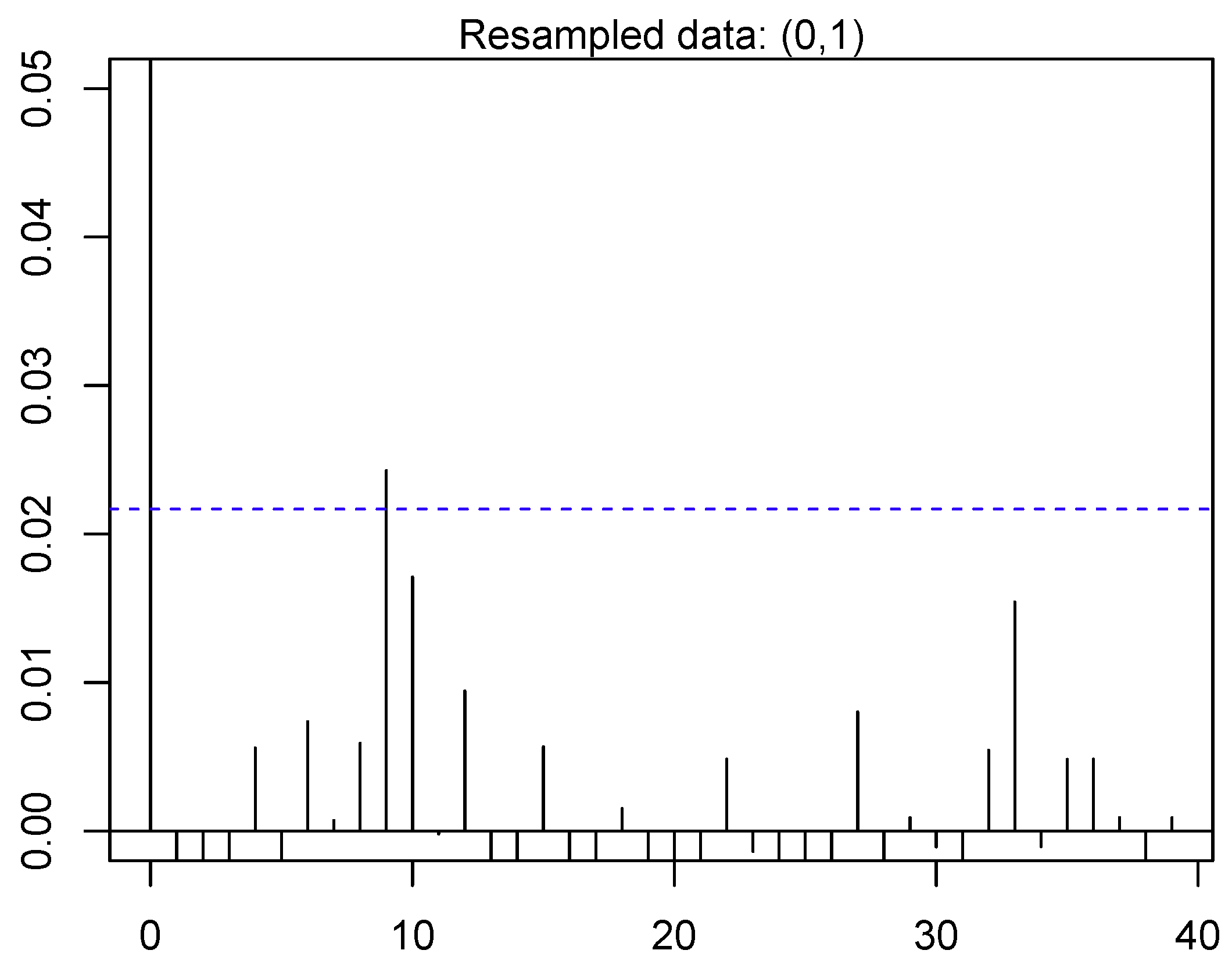
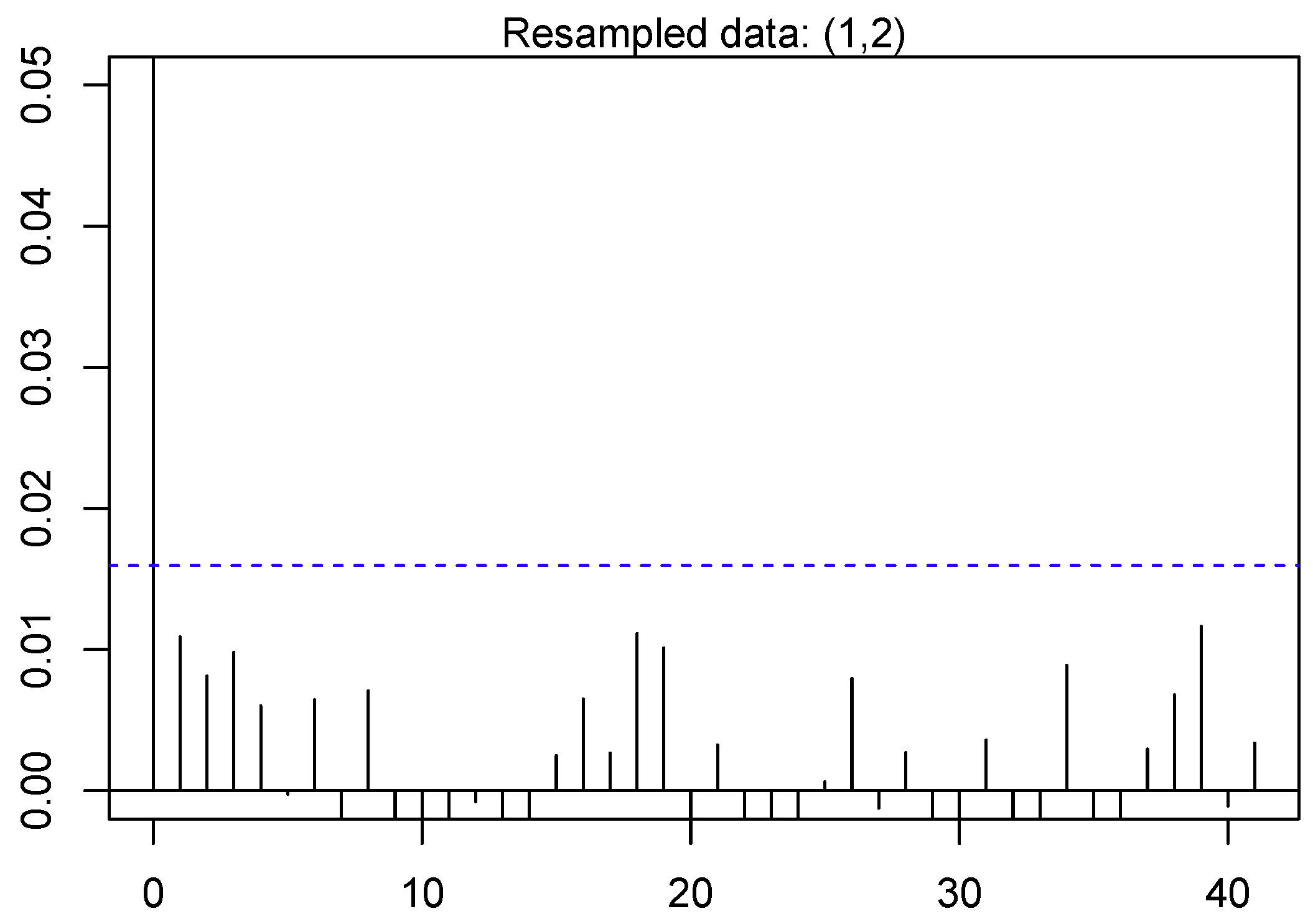
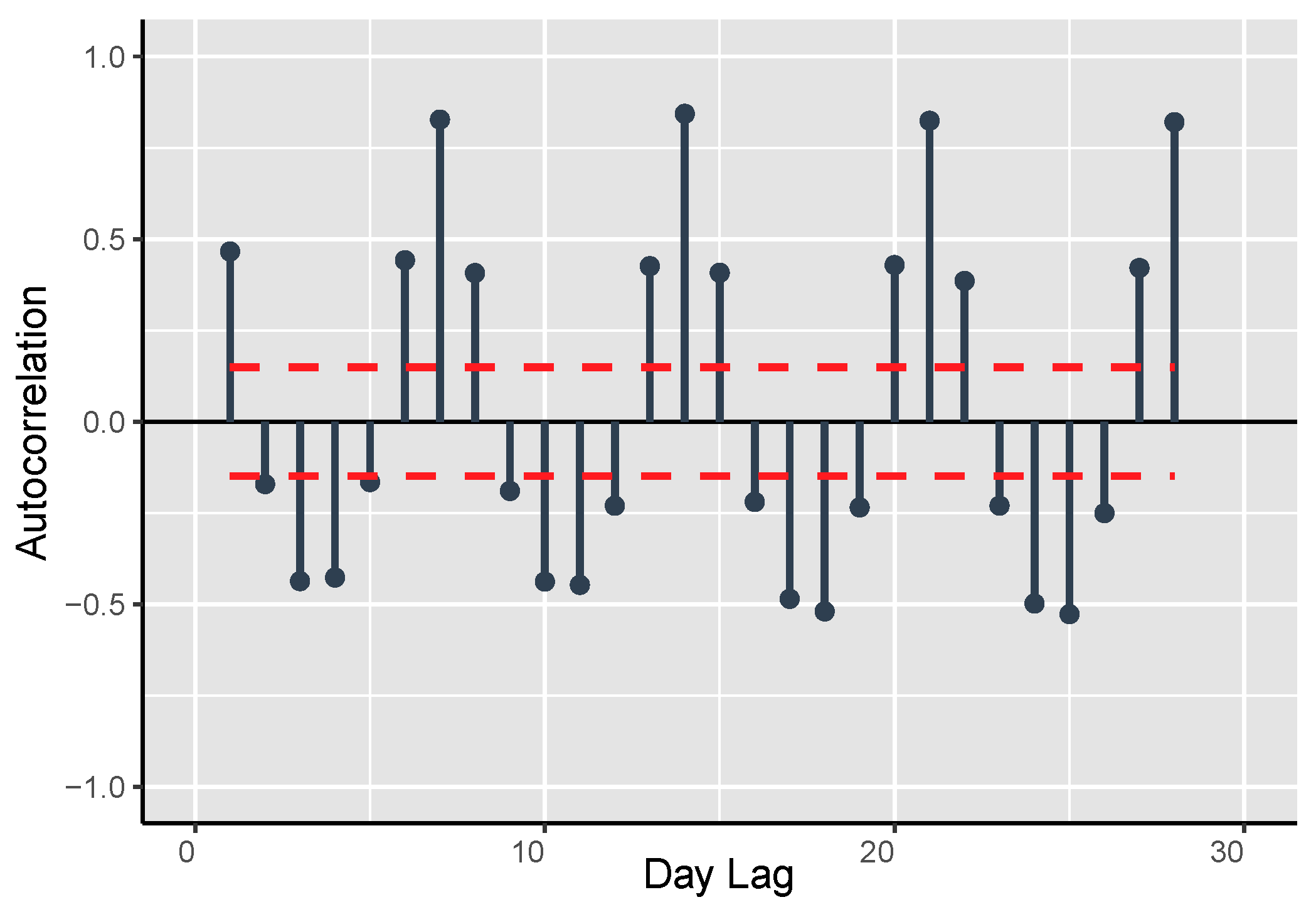
Figure 10 for the previous data. It is obvious from the auto-correlation plots that the preceding data is more auto-correlated to experimental data, to some extent. This paper performs Ljung Box [78] analysis of null supposition to check this assumption more quantitively. The suppositions are as follows:
  • S 0 : The preceding data are disseminated autonomously, i.e., the correlation is 0 in the preceding data from where the sample is chosen. Therefore, any experimental correlations in the preceding data are the resultant from the unpredictability of the test group.
  • S 1 : The preceding data are not disseminated autonomously, i.e., the data show serial correlation.
The auto-correlations tests are performed whose outcomes are shown in Table 4.
The outcomes show that the preceding data is much more auto-correlated as compared to the experimental data. It is often observed in literature that numerous testing process reject the S 0 for the preceding data. However, S 0 is not rejected by experimental data. Therefore, there subsists a spatial correlation in preceding data. Moreover, if sampling techniques are applied on the historic data then this correlation can be disintegrated. The paper also performs sensitivity analysis and the structure of DBN used for this paper includes one hidden layer with five neurons. Moreover, there are 25 neurons are in input layer and 20 neurons in the output layer in the proposed architecture. These neurons generate the prediction of load demand for the target day (24 h). On the topic of architecture of this network, the input layer is comprised of two constraints for mean and maximum temperature for selected day. Moreover, one constraint is for categorization of the forecasted day while the remaining 22 input constraints are associated with the preceding load demand data, which are as follows:
ϱ τ = Γ m τ Γ n τ Γ n τ .
In Equation (48), ϱ τ represents the total load demand data, Γ m τ and Γ n τ are demand load for τ t h hour ( τ = 1 , 2 , 3 , , 24 ) preceding to selected day. This paper assumes that Γ m τ and Γ n τ represents the τ and τ -1 hours in Equation (48). Moreover, there are 20 neurons in the output ( OS τ ) layer of DBN that signifies the difference of load demand on the hourly basis for preceding and selected days,
OS τ = Γ t a r τ Γ n τ Γ n τ .
The categorization of days in DBN are entirely divergent from knowledge based system. According to Equations (48) and (49), Tuesday must be taken apart from days that range from Wednesday to Friday. Therefore, in DBN five categories of days are taken for analysis.

5.2. Fuzzy Local Linear Model Tree Algorithm

The paper employs F-LOLIMOT algorithm for training of the linear fuzzy model. The explanatory analysis of F-LOLIMOT algorithm has been discussed in detail in [79]. Moreover, the F-LOLIMOT algorithm is capable of predicting the hourly demand load, which is ahead than the current time by means of climatic and load data. Figure 11 depicts that there are different inputs and outputs of demand load and climatic data. This is done after sensitivity analysis on the system.
Furthermore, the lags of climate are the climatic condition of the preceding week and target day. Likewise, the time lags of each hour load demand (inputs) are actually demand load data of similar hour at preceding 9 and 10 days earlier than selected hour. It is obvious that the initial hour of target day by utilizing preceding and recognized load data the upcoming hourly load is forecasted by preceding data.

6. Results and Discussion

At first, this section presents the evaluational measures that are used in this paper. Subsequently, the results are discussed.

6.1. Evaluational Measures

In literature, Daily Maximum Error (DME), Maximum Distance Minimum Error (MDME), and MAPE have been widely used in order to valuate the outcomes, which are achieved from short-term forecasting. This paper has used MAPE, MDME and DME as:
M A P E = D f 1 D f H = 1 Γ t a r , H Γ ν , H Γ ν , H
and
D M E = m a x ( Γ t a r , H Γ ν , H Γ ν , H ) .
In Equations (50) and (51), D f are the hours that are forecasted and Γ ν , H is the real demand load at specified hour H of tar day. This paper presents 4 implications to indicate the benefits of the proposed system. The implications are based on the forecasting of load demand for the duration of June 2015 to June 2016. Moreover, these implications are made by climatic and load data, which lies in the range of June 2015 to exactly one day before the target day. The paper takes this data as training data in this scenario. The implications are:
  • MAPE of short-term load forecasting throughout the year ( D f = 9750)
  • Average of DME throughout the year, which is referred as maximum distance and minimum error
  • Total number of days, which have MAPE higher than 3% ( 3 )
  • Total number of days, which have maximum error higher than 5% ( 5 )
The last two implications depict the division of errors, which are achieved from the results of short-term load forecasting. In this paper, the proposed model minimizes the total number of exceeding days from a certain limit and also enhances the performance of MAPE and DME.

6.2. Discussion of Results

The paper has evaluated the results on the basis of two assumed evaluations that are discussed as follows.

6.2.1. Evaluation of Priority Index and Splitting Consequences on Knowledge Based Systems

This paper implements the proposed method on PNPN. In this regard, the following cases are observed to discuss the consequences, which are associated with distribution of the forecasting results and taking temperature in priority index.
  • Case 1: Short-term load forecasting of PNPN without taking temperature and distribution of data
  • Case 2: Short-term load forecasting of PNPN including consequences of data distribution without taking the temperature
  • Case 3: Short-term load forecasting of PNPN including including temperature without taking the consequences of data distribution
  • Case 4: Short-term load forecasting of PNPN with temperature and distribution of data
The data distribution is overlooked in Case 1. Therefore, a distinctive temperature is not suitable for the system. Moreover, the priority index is the center of attention in this case along with the date proximity. Besides, the whole system is distributed in different sections in Case 2. Subsequently, the prediction is performed for every respective section. The prediction of the entire system is a combination of predicting outcomes in all sections. Case 2 differs from Case 1 as the data distribution is carried out in this scenario. Nonetheless, the data distribution is also overlooked in Case 3. However, the temperature is taken in consideration in terms of subjective average values in relation to the demand from every region. The consequences of temperature are studied in Case 4. The paper assumes Case 4 as a comprehensive case as it takes temperature in the priority index for selection of similar days from every section.
Table 5 and Table 6 presents the outcomes of the aforementioned cases for every category of the day. It can be observed that MAPE of the entire system is minimum in Case 4 as compared to other cases. The data distribution is done in Case 2 and Case 1 has overlooked this phenomenon. Thus, it is proved that distributing the entire system can enhance the prediction outcomes. Moreover, the data distribution also minimizes the MAPE and maximum distance and minimum error. Besides, the data distribution among different regions minimizes the total number of days that go beyond acceptable measures ( 3 and 5 ).
The consideration of temperature devoid of distributing the data in different regions is responsible for reduction in valuation constraints when associated with Case 1 and Case 2. Nevertheless, the MAPE of Case 4 is enhanced as compared to Case 3. Moreover, Case 4 has minimum days with maximum error that is larger than 4%. Contrariwise, forecasting results are improved in Case 4 as it distributes the data in different regions and takes temperature in priority index. The MAPE in Case 4 is 1.02 % as depicted in Table 5 and Table 6. This achieved MAPE is approximately 8% improved than Case 2 and almost 9% enhanced than Case 1. Besides, Case 4 has the total number of optimum days that exceeds the acceptable criteria. The results achieved for minimum days with maximum error and 5 are also enhanced in Case 4 as compared to Case 3. Nonetheless, 3 has achieved enhanced results in Case 3 in comparison with Case 4.
Table 7 presents D γ and W 1 for target year. The optimum result achieved is for D γ = 7 and W 1 = 0.3. The results achieved for W 1 = 0.3 are approximately near to W 1 = 0.4. Thus, the achieved parameters from training data can give suitable outcomes and are proven appropriate for the proposed method.

6.2.2. Evaluation of Consequences on knowledge Based Systems from Preceding Data

The preceding data is categorized in two different sets as discussed in Section II. The paper studies three cases in this subsection to depict the consequences of this type of categorization.
  • Case 1: Load forecasting by collected similar days in initial data-set, Γ t a r , H d s 1
  • Case 2: Load forecasting by collected similar days in last data-set, Γ t a r , H d s 2
  • Case 3: Load forecasting by Γ t a r , H d s 1 and Γ t a r , H d s 2 , i.e., Γ t a r , H Equation (44)
Table 8 presents the outcomes of Case 1, Case 2, and Case 3 for every category of the day. Table 8 presents the outcomes of Case 1, Case 2, and Case 3 for every category of the day.
The MAPE of the entire system in Case 1 is maximum as compared to Case 2 and Case 3 in case of Γ t a r , H d s 1 . Thus, it can be concluded that taking same days from selected or last month gives maximum errors in forecasting results. Moreover, the total number of exceeding days from acceptable conditions is not suitable, particularly 5 . Nevertheless, integration of Γ t a r , H d s 1 and Γ t a r , H d s 2 gives enhanced results for MAPE and minimum days with maximum error in Case 3. Furthermore, passed days from acceptable conditions is lessened in Case 3.
Figure 12, Figure 13 and Figure 14 depicts the comparative analysis of traditional and proposed forecasting method. According to Figure 12, Figure 13 and Figure 14, the days presented are four different days and these days belong to dissimilar months. The predicted outcomes are then associated with real load demand. Moreover, the results of the proposed system are much nearer to real load as compared to traditional forecasting techniques.

6.3. Comparative Analysis of Proposed Method, DBN, and F-LOLIMOT

The paper compares the results achieved from proposed knowledge based system with DBN and F-LOLIMOT. The results are evaluated in terms of precision and operational time. The short-term load predicting techniques is applied on PNPN to forecast the load demand for the duration of June 2017 to May 2018. Moreover, these predictions are based on temperature and load demand data, which lies in the range of June 2015 to exactly one day before the target day. The results are presented in Table 9, which shows that proposed knowledge based system has enhanced MAPE to 1.01. Besides, the MAPE of 5 and 5 is also decreased. The DBN and F-LOLIMOT techniques show MAPE is approximately higher than 3% for a month and approximately 5% greater in 47–50 days (maximum error). Nonetheless, the proposed method has MAPE, which is greater than 3% in 15–18 days and 5% with 23 days (maximum error). The variances discussed are notable enhancements in forecasting.
On the topic of operational cost, the proposed knowledge based method takes minimum time in training and executing in comparison with DBN and F-LOLIMOT. The proposed knowledge based system, DBN, and F-LOLIMOT are executed to predict the days on a yearly basis. Besides, the operational time is distributed to total number of predicted days in order to get the usual operational time of prediction for a specified day. Moreover, the proposed system, DBN, and F-LOLIMOT are executed with the same conditions. Besides, the parameters were tuned for every specified day and forecasted demand load has been achieved for every technique. The paper distributes the day, according to training and operational time in every technique. The proposed knowledge base systems have less operational time as it does not require as much training as compared to DBN and F-LOLIMOT. The proposed method lays emphasis on the selection of similar day and then predicts the load demand as discussed above.
The forecasting of sample day is presented in Figure 15 and Figure 16 by means of DBN, F-LOLIMOT, and proposed knowledge based system. It is obvious that MAPE of the proposed method is 0.69 for a sample day. This MAPE is lesser than MAPEs of DBN and F-LOLIMOT, which are 0.91 and 0.97 respectively. Moreover, the DME is minimized in the presented knowledge based system as compared to others. The phenomenon of priority index is not suitable for special days (public holidays) as discussed in earlier sections. Nevertheless, the special days can be forecasted by the presented knowledge based system devoid of taking a priority index. Besides, the MAPE of the proposed system is 1.30 for all days, together with special days. Nonetheless, the major aim of this paper is to study the consequences of the priority index on the knowledge based system. Moreover, the scrutiny of special days is beyond the scope of this paper.

7. Conclusions

This paper presents a novel knowledge based short-term load forecasting method. The entire system (region) is distributed in nine sub-systems (zones) by consideration of temperature to predict the demand load more efficiently. The outcomes depict that distribution of huge topographical power network improves the forecasting results. Moreover, this paper presents a novel priority index in which climatic conditions and the date proximity of every particular region is observed. The algorithms of AP and BFFA are hybridized in this paper to achieve better accuracy for a knowledge based system. The proposed knowledge based system is verified on PNPN. The achieved outcomes depict that proposed method minimizes the MAPE and other errors of forecasting in comparison with traditional forecasting techniques. Furthermore, the obtained results from proposed system are 15–20% improved as compared to DBN and F-LOLIMOT techniques. Furthermore, this paper defines two standard measures for error distribution. The outcomes verify that the total amount of exceeded days is reduced through proposing knowledge based systems from acceptable criteria. This phenomenon specifies more efficient forecasting results as compared to DBN, F-LOLIMOT, and traditional knowledge based systems.

Author Contributions

All authors have contributed to this paper with the same effort in finding available literature, resources and writing the paper. Moreover, all authors have read and approved the final manuscript.

Funding

This research received no external funding.

Conflicts of Interest

The authors declare no conflict of interest.

References

  1. Schleicher-Tappeser, R. How renewables will change electricity markets in the next five years. Energy Policy 2012, 48, 64–75. [Google Scholar] [CrossRef]
  2. Farhangi, H. The path of the smart grid. IEEE Power Energy Mag. 2010, 8, 18–28. [Google Scholar] [CrossRef]
  3. Zipperer, A.; Aloise-Young, P.A.; Suryanarayanan, S.; Roche, R.; Earle, L.; Christensen, D.; Bauleo, P.; Zimmerle, D. Electric Energy Management in the Smart Home: Perspectives on Enabling Technologies and Consumer Behavior. Proc. IEEE 2013, 101, 2397–2408. [Google Scholar] [CrossRef]
  4. Beaudin, M.; Zareipour, H. Home energy management systems: A review of modelling and complexity. Renew. Sustain. Energy Rev. 2015, 45, 318–335. [Google Scholar] [CrossRef]
  5. Luo, X.; Wang, J.; Dooner, M.; Clarke, J. Overview of current development in electrical energy storage technologies and the application potential in power system operation. Appl. Energy 2015, 137, 511–536. [Google Scholar] [CrossRef]
  6. Pothitou, M.; Hanna, R.F.; Chalvatzis, K.J. Environmental knowledge, pro-environmental behaviour and energy savings in households: An empirical study. Appl. Energy 2016, 184, 1217–1229. [Google Scholar] [CrossRef] [Green Version]
  7. O’Neill, R.P.; Sotkiewicz, P.M.; Hobbs, B.F.; Rothkopf, M.H.; Stewart, W.R. Efficient market-clearing prices in markets with nonconvexities. Eur. J. Oper. Res. 2005, 164, 269–285. [Google Scholar] [CrossRef] [Green Version]
  8. Ghasemi, A.; Mortazavi, S.S.; Mashhour, E. Hourly demand response and battery energy storage for imbalance reduction of smart distribution company embedded with electric vehicles and wind farms. Renew. Energy 2016, 85, 124–136. [Google Scholar] [CrossRef]
  9. Azizipanah-Abarghooee, R.; Terzija, V.; Golestaneh, F.; Roosta, A. Multiobjective Dynamic Optimal Power Flow Considering Fuzzy-Based Smart Utilization of Mobile Electric Vehicles. IEEE Trans. Ind. Inform. 2016, 12, 503–514. [Google Scholar] [CrossRef]
  10. Khan, M.; Javaid, N.; Iqbal, M.N.; Bilal, M.; Zaidi, S.F.A.; Raza, R.A. Load Prediction Based on Multivariate Time Series Forecasting for Energy Consumption and Behavioral Analytics. In Proceedings of the Conference on Complex, Intelligent, and Software Intensive Systems, Matsue, Japan, 4–6 July 2018; Springer: Cham, Switzerland, 2018; pp. 305–316. [Google Scholar]
  11. Rahim, S.; Javaid, N.; Ahmad, A.; Khan, S.A.; Khan, Z.A.; Alrajeh, N.; Qasim, U. Exploiting heuristic algorithms to efficiently utilize energy management controllers with renewable energy sources. Energy Build. 2016, 129, 452–470. [Google Scholar] [CrossRef]
  12. Zhu, G.; Chow, T.T.; Tse, N. Short-term load forecasting coupled with weather profile generation methodology. Build. Serv. Eng. Res. Technol. 2018, 39, 310–327. [Google Scholar] [CrossRef]
  13. Ahmad, A.; Javaid, N.; Guizani, M.; Alrajeh, N.; Khan, Z.A. An Accurate and Fast Converging Short-Term Load Forecasting Model for Industrial Applications in a Smart Grid. IEEE Trans. Ind. Inform. 2017, 13, 2587–2596. [Google Scholar] [CrossRef]
  14. Ahmad, T.; Chen, H.; Huang, R.; Yabin, G.; Wang, J.; Shair, J.; Azeem Akram, H.M.; Hassnain Mohsan, S.A.; Kazim, M. Supervised based machine learning models for short, medium and long-term energy prediction in distinct building environment. Energy 2018, 158, 17–32. [Google Scholar] [CrossRef]
  15. Lima, F.J.; Martins, F.R.; Pereira, E.B.; Lorenz, E.; Heinemann, D. Forecast for surface solar irradiance at the Brazilian Northeastern region using NWP model and artificial neural networks. Renew. Energy 2016, 87, 807–818. [Google Scholar] [CrossRef]
  16. Vrbsky, L.; da Silva, M.S.; Cardoso, D.L.; Frances, C.R.L. Clustering techniques for data network planning in Smart Grids. In Proceedings of the IEEE 14th International Conference on Networking, Sensing and Control (ICNSC), Calabria, Italy, 16–18 May 2017; pp. 7–12. [Google Scholar] [CrossRef]
  17. Muratori, M.; Rizzoni, G. Residential Demand Response: Dynamic Energy Management and Time-Varying Electricity Pricing. IEEE Trans. Power Syst. 2016, 31, 1108–1117. [Google Scholar] [CrossRef]
  18. Silva, G.C.; Silva, J.L.R.; Lisboa, A.C.; Vieira, D.A.G.; Saldanha, R.R. Advanced fuzzy time series applied to short term load forecasting. In Proceedings of the IEEE Latin American Conference on Computational Intelligence (LA-CCI), Arequipa, Peru, 8–10 November 2017; pp. 1–6. [Google Scholar] [CrossRef]
  19. Mayrink, V.; Hippert, H.S. A hybrid method using Exponential Smoothing and Gradient Boosting for electrical short-term load forecasting. In Proceedings of the IEEE Latin American Conference on Computational Intelligence (LA-CCI), Cartagena, Colombia, 2–4 November 2016; pp. 1–6. [Google Scholar] [CrossRef]
  20. He, Y.; Xu, Q.; Wan, J.; Yang, S. Short-term power load probability density forecasting based on quantile regression neural network and triangle kernel function. Energy 2016, 114, 498–512. [Google Scholar] [CrossRef]
  21. Li, S.; Wang, P.; Goel, L. A novel wavelet-based ensemble method for short-term load forecasting with hybrid neural networks and feature selection. IEEE Trans. Power Syst. 2016, 31, 1788–1798. [Google Scholar] [CrossRef]
  22. Wang, J.; Hu, J. A robust combination approach for short-term wind speed forecasting and analysis—A robust combination approach for short-term wind speed forecasting and analysis—Combination of the ARIMA (Autoregressive Integrated Moving Average), ELM (Extreme Learning Machine), SVM (Support Vector Machine) and LSSVM (Least Square SVM) forecasts using a GPR (Gaussian Process Regression) model. Energy 2015, 93, 41–56. [Google Scholar]
  23. Jackson, E.A. Comparison between Static and Dynamic Forecast in Autoregressive Integrated Moving Average for Seasonally Adjusted Headline Consumer Price Index. SSRN Electron. J. 2018, 1–14. [Google Scholar] [CrossRef]
  24. Mitchell, G.; Bahadoorsingh, S.; Ramsamooj, N.; Sharma, C. A comparison of artificial neural networks and support vector machines for short-term load forecasting using various load types. In Proceedings of the IEEE Manchester PowerTech, Manchester, UK, 18–22 June 2017; pp. 1–4. [Google Scholar]
  25. Di Persio, L.; Cecchin, A.; Cordoni, F. Novel approaches to the energy load unbalance forecasting in the Italian electricity market. J. Math. Ind. 2017. [Google Scholar] [CrossRef]
  26. Barman, M.; Dev Choudhury, N.; Sutradhar, S. A regional hybrid GOA-SVM model based on similar day approach for short-term load forecasting in Assam, India. Energy 2018, 145, 710–720. [Google Scholar] [CrossRef]
  27. Sepasi, S.; Reihani, E.; Howlader, A.M.; Roose, L.R.; Matsuura, M.M. Very short term load forecasting of a distribution system with high PV penetration. Renew. Energy 2017, 106, 142–148. [Google Scholar] [CrossRef]
  28. Eapen, R.R.; Simon, S.P. Performance Analysis of Combined Similar Day and Day Ahead Short Term Electrical Load Forecasting using Sequential Hybrid Neural Networks. IETE J. Res. 2018. [Google Scholar] [CrossRef]
  29. Ahmad, A.; Anderson, T.N.; Rehman, S.U. Prediction of Electricity Consumption for Residential Houses in New Zealand; Springer: Cham, Switzerland, 2018; pp. 165–172. [Google Scholar]
  30. Hoverstad, B.A.; Tidemann, A.; Langseth, H.; Ozturk, P. Short-Term Load Forecasting With Seasonal Decomposition Using Evolution for Parameter Tuning. IEEE Trans. Smart Grid 2015, 6, 1904–1913. [Google Scholar] [CrossRef]
  31. Kavanagh, K.; Barrett, M.; Conlon, M. Short-term electricity load forecasting for the integrated single electricity market (I-SEM). In Proceedings of the 52nd International Universities Power Engineering Conference (UPEC), Heraklion, Greece, 28–31 August 2017; pp. 1–7. [Google Scholar] [CrossRef]
  32. Alobaidi, M.H.; Chebana, F.; Meguid, M.A. Robust ensemble learning framework for day-ahead forecasting of household based energy consumption. Appl. Energy 2018, 212, 997–1012. [Google Scholar] [CrossRef]
  33. Lydia, M.; Suresh Kumar, S.; Immanuel Selvakumar, A.; Edwin Prem Kumar, G. Linear and non-linear autoregressive models for short-term wind speed forecasting. Energy Convers. Manag. 2016, 112, 115–124. [Google Scholar] [CrossRef]
  34. Bramer, L.; Rounds, J.; Burleyson, C.; Fortin, D.; Hathaway, J.; Rice, J.; Kraucunas, I. Evaluating penalized logistic regression models to predict Heat-Related Electric grid stress days. Appl. Energy 2017, 205, 1408–1418. [Google Scholar] [CrossRef]
  35. Yukseltan, E.; Yucekaya, A.; Bilge, A.H. Forecasting electricity demand for Turkey: Modeling periodic variations and demand segregation. Appl. Energy 2017, 193, 287–296. [Google Scholar] [CrossRef]
  36. Abdoos, A.; Hemmati, M.; Abdoos, A.A. Short term load forecasting using a hybrid intelligent method. Knowl.-Based Syst. 2015, 76, 139–147. [Google Scholar] [CrossRef]
  37. Carvallo, J.P.; Larsen, P.H.; Sanstad, A.H.; Goldman, C.A. Long term load forecasting accuracy in electric utility integrated resource planning. Energy Policy 2018, 119, 410–422. [Google Scholar] [CrossRef]
  38. Hawarah, L.; Ploix, S.; Jacomino, M. User Behavior Prediction in Energy Consumption in Housing Using Bayesian Networks; Springer: Berlin/Heidelberg, Germany, 2010; pp. 372–379. [Google Scholar]
  39. Basu, K.; Debusschere, V.; Bacha, S. Appliance usage prediction using a time series based classification approach. In Proceedings of the IECON 2012—38th Annual Conference on IEEE Industrial Electronics Society, Montreal, QC, Canada, 25–28 October 2012; pp. 1217–1222. [Google Scholar] [CrossRef]
  40. Basu, K.; Hawarah, L.; Arghira, N.; Joumaa, H.; Ploix, S. A prediction system for home appliance usage. Energy Build. 2013, 67, 668–679. [Google Scholar] [CrossRef]
  41. Rollins, S.; Banerjee, N. Using rule mining to understand appliance energy consumption patterns. In Proceedings of the IEEE International Conference on Pervasive Computing and Communications (PerCom), Budapest, Hungary, 24–28 March 2014; pp. 29–37. [Google Scholar] [CrossRef]
  42. Karatasou, S.; Santamouris, M.; Geros, V. Modeling and predicting building’s energy use with artificial neural networks: Methods and results. Energy Build. 2006, 38, 949–958. [Google Scholar] [CrossRef]
  43. Chen, Y.; Yang, Y.; Liu, C.; Li, C.; Li, L. A hybrid application algorithm based on the support vector machine and artificial intelligence: An example of electric load forecasting. Appl. Math. Model. 2015, 39, 2617–2632. [Google Scholar] [CrossRef]
  44. Hong, W.C. Electric load forecasting by support vector model. Appl. Math. Model. 2009, 33, 2444–2454. [Google Scholar] [CrossRef]
  45. Zhao, H.X.; Magoulès, F. A review on the prediction of building energy consumption. Renew. Sustain. Energy Rev. 2012, 16, 3586–3592. [Google Scholar] [CrossRef]
  46. Li, X.; Lu, J.; Ding, L.; Xu, G.; Li, J. Building Cooling Load Forecasting Model Based on LS-SVM. In Proceedings of the 2009 Asia-Pacific Conference on Information Processing, Shenzhen, China, 18–19 July 2009; pp. 55–58. [Google Scholar]
  47. Li, H.Z.; Guo, S.; Li, C.J.; Sun, J.Q. A hybrid annual power load forecasting model based on generalized regression neural network with fruit fly optimization algorithm. Knowl.-Based Syst. 2013, 37, 378–387. [Google Scholar] [CrossRef]
  48. Wang, J.; Li, L.; Niu, D.; Tan, Z. An annual load forecasting model based on support vector regression with differential evolution algorithm. Appl. Energy 2012, 94, 65–70. [Google Scholar] [CrossRef]
  49. Faris, H.; Hassonah, M.A.; Al-Zoubi, A.M.; Mirjalili, S.; Aljarah, I. A multi-verse optimizer approach for feature selection and optimizing SVM parameters based on a robust system architecture. Neural Comput. Appl. 2018, 30, 2355–2369. [Google Scholar] [CrossRef]
  50. Ogliari, E.; Grimaccia, F.; Leva, S.; Mussetta, M.; Ogliari, E.; Grimaccia, F.; Leva, S.; Mussetta, M. Hybrid Predictive Models for Accurate Forecasting in PV Systems. Energies 2013, 6, 1918–1929. [Google Scholar] [CrossRef] [Green Version]
  51. Geng, J.; Huang, M.L.; Li, M.W.; Hong, W.C. Hybridization of seasonal chaotic cloud simulated annealing algorithm in a SVR-based load forecasting model. Neurocomputing 2015, 151, 1362–1373. [Google Scholar] [CrossRef]
  52. Bedekar, P.P.; Korde, P.N. Determining optimum time multiplier setting of overcurrent relays using modified Jaya algorithm. In Proceedings of the 2017 Innovations in Power and Advanced Computing Technologies (i-PACT), Vellore, India, 21–22 April 2017; pp. 1–6. [Google Scholar] [CrossRef]
  53. Samuel, O.; Javaid, N.; Ashraf, M.; Ishmanov, F.; Afzal, M.; Khan, Z. Jaya based Optimization Method with High Dispatchable Distributed Generation for Residential Microgrid. Energies 2018, 11, 1513. [Google Scholar] [CrossRef]
  54. Mohsenian Rad, A.H.; Wong, V.W.S.; Jatskevich, J.; Schober, R.; Leon Garcia, A. Autonomous Demand-Side Management Based on Game-Theoretic Energy Consumption Scheduling for the Future Smart Grid. IEEE Trans. Smart Grid 2010, 1, 320–331. [Google Scholar] [CrossRef] [Green Version]
  55. Siano, P. Demand response and smart grids—A survey. Renew. Sustain. Energy Rev. 2014, 30, 461–478. [Google Scholar] [CrossRef]
  56. Wang, H.; Huang, J. Joint investment and operation of microgrid. IEEE Trans. Smart Grid 2017, 8, 833–845. [Google Scholar] [CrossRef]
  57. Siano, P.; Sarno, D. Assessing the benefits of residential demand response in a real time distribution energy market. Appl. Energy 2016, 161, 533–551. [Google Scholar] [CrossRef]
  58. Liu, Y.; Yuen, C.; Yu, R.; Zhang, Y.; Xie, S. Queuing-Based Energy Consumption Management for Heterogeneous Residential Demands in Smart Grid. IEEE Trans. Smart Grid 2016, 7, 1650–1659. [Google Scholar] [CrossRef]
  59. Zhou, B.; Li, W.; Chan, K.W.; Cao, Y.; Kuang, Y.; Liu, X.; Wang, X. Smart home energy management systems: Concept, configurations, and scheduling strategies. Renew. Sustain. Energy Rev. 2016, 61, 30–40. [Google Scholar] [CrossRef]
  60. Marcon, P.; Szabo, Z.; Vesely, I.; Zezulka, F.; Sajdl, O.; Roubal, Z.; Dohnal, P. A Real Model of a Micro-Grid to Improve Network Stability. Appl. Sci. 2017, 7, 757. [Google Scholar] [CrossRef]
  61. Liu, Y.; Li, T.; Chen, Y.; Wang, D.; Liu, Y.; Li, T.; Chen, Y.; Wang, D. Optimization of Solar Water Heating System under Time and Spatial Partition Heating in Rural Dwellings. Energies 2017, 10, 1561. [Google Scholar] [CrossRef]
  62. Esther, B.P.; Kumar, K.S. A survey on residential Demand Side Management architecture, approaches, optimization models and methods. Renew. Sustain. Energy Rev. 2016, 59, 342–351. [Google Scholar] [CrossRef]
  63. Alshehri, K.; Liu, J.; Chen, X.; Basar, T. A Stackelberg game for multi-period demand response management in the smart grid. In Proceedings of the 54th IEEE Conference on Decision and Control (CDC), Osaka, Japan, 15–18 December 2015; pp. 5889–5894. [Google Scholar]
  64. Liang, H.; Tamang, A.K.; Zhuang, W.; Shen, X.S. Stochastic Information Management in Smart Grid. IEEE Commun. Surv. Tutor. 2014, 16, 1746–1770. [Google Scholar] [CrossRef]
  65. Luo, X.; Lee, C.K.; Ng, W.M.; Yan, S.; Chaudhuri, B.; Hui, S.Y.R. Use of Adaptive Thermal Storage System as Smart Load for Voltage Control and Demand Response. IEEE Trans. Smart Grid 2017, 8, 1231–1241. [Google Scholar] [CrossRef]
  66. Lee, J.; Guo, J.; Choi, J.K.; Zukerman, M. Distributed Energy Trading in Microgrids: A Game Theoretic Model and Its Equilibrium Analysis. IEEE Trans. Ind. Electron. 2015, 62, 3524–3533. [Google Scholar] [CrossRef]
  67. Erol-Kantarci, M.; Mouftah, H.T. Energy-Efficient Information and Communication Infrastructures in the Smart Grid: A Survey on Interactions and Open Issues. IEEE Commun. Surv. Tutor. 2015, 17, 179–197. [Google Scholar] [CrossRef]
  68. Carnicer, J.M.; Goodman, T.N.T.; Peña, J.M. Linear conditions for positive determinants. Linear Algebra Its Appl. 1999, 292, 39–59. [Google Scholar] [CrossRef]
  69. Chai, B.; Chen, J.; Yang, Z.; Zhang, Y. Demand Response Management With Multiple Utility Companies: A Two-Level Game Approach. IEEE Trans. Smart Grid 2014, 5, 722–731. [Google Scholar] [CrossRef]
  70. Emami, N.; Pakzad, A. A New Knowledge-Based System for Diagnosis of Breast Cancer by a combination of the Affinity Propagation and Firefly Algorithms; Shahrood University of Technology: Shahrood, Iran, 2018. [Google Scholar]
  71. GhaffarianHoseini, A.; Zhang, T.; Nwadigo, O.; GhaffarianHoseini, A.; Naismith, N.; Tookey, J.; Raahemifar, K. Application of nD BIM Integrated Knowledge-based Building Management System (BIM-IKBMS) for inspecting post-construction energy efficiency. Renew. Sustain. Energy Rev. 2017, 72, 935–949. [Google Scholar] [CrossRef] [Green Version]
  72. Lin, J.; Wang, F.; Cai, A.; Yan, W.; Cui, W.; Mo, J. Daily Load Curve Forecasting Using Factor Analysis and RBF Neural Network Based on Load Segmentation. In Proceedings of the China International Electrical and Energy Conference (CIEEC), Beijing, China, 19–21 October 2017; pp. 601–606. [Google Scholar]
  73. Ashouri, M.; Haghighat, F.; Fung, B.C.; Lazrak, A.; Yoshino, H. Development of building energy saving advisory: A data mining approach. Energy Build. 2018, 172, 139–151. [Google Scholar] [CrossRef]
  74. Raza, M.Q.; Nadarajah, M.; Hung, D.Q.; Baharudin, Z. An intelligent hybrid short-term load forecasting model for smart power grids. Sustain. Cities Soc. 2017, 31, 264–275. [Google Scholar] [CrossRef]
  75. Golestaneh, F.; Pinson, P.; Gooi, H.B. Very Short-Term Nonparametric Probabilistic Forecasting of Renewable Energy Generation; With Application to Solar Energy. IEEE Trans. Smart Grids 2016, 31, 3850–3863. [Google Scholar] [CrossRef]
  76. Cerne, G.; Dovzan, D.; Skrjanc, I. Short-term load forecasting by separating daily profile and using a single fuzzy model across the entire domain. IEEE Trans. Ind. Electron. 2018, 65, 7406–7415. [Google Scholar] [CrossRef]
  77. Dedinec, A.; Filiposka, S.; Dedinec, A.; Kocarev, L. Deep belief network based electricity load forecasting: An analysis of Macedonian case. Energy 2016, 115, 1688–1700. [Google Scholar] [CrossRef]
  78. Guarnaccia, C.; Tepedino, C.; Iliev, S.; Popova, S.; Quartieri, J. A Forecasting Model Based on Time Series Analysis Applied to Electrical Energy Consumption. Int. J. Math. Models Methods Appl. Sci. 2015, 9, 432. [Google Scholar]
  79. Dong, Q.; Sun, Y.; Li, P. A novel forecasting model based on a hybrid processing strategy and an optimized local linear fuzzy neural network to make wind power forecasting: A case study of wind farms in China. Renew. Energy 2017, 102, 241–257. [Google Scholar] [CrossRef]
Figure 1. Principle components of knowledge based system.
Electronics 07 00431 g001
Figure 2. Variations in load behavior of sample Thursday during 2015 of Pakistan’s National Power Network (PNPN).
Electronics 07 00431 g002
Figure 3. Heatmap and yearly weather conditions of sample region.
Electronics 07 00431 g003
Figure 4. Variations of temperature for average mid-day weather of Lahore.
Electronics 07 00431 g004
Figure 5. Fluctuating Behavior of Load Curve in Pakistan and Difference of Monday and a Sample Week-day.
Electronics 07 00431 g005
Figure 6. Fluctuating behavior of load curve in Pakistan of a particular week.
Electronics 07 00431 g006
Figure 7. Auto-correlation of preceding demand load data for day lags in deep belief network (DBN) for original data (0, 1).
Electronics 07 00431 g007
Figure 8. Auto-correlation of preceding demand load data for day lags in DBN for original data (0, 1).
Electronics 07 00431 g008
Figure 9. Auto-correlation of preceding demand load data for day lags in DBN for original data (1, 2).
Electronics 07 00431 g009
Figure 10. Auto-correlation of preceding demand load data for day lags in DBN for resampled data (1,2).
Electronics 07 00431 g010
Figure 11. Auto-correlation of preceding demand load data for day lags in Fuzzy Local Linear Model Tree (F-LOLIMOT).
Electronics 07 00431 g011
Figure 12. Comparative analysis and effect of proposed and traditional method for Monday, 19 September 2015.
Electronics 07 00431 g012
Figure 13. Comparative analysis and effect of proposed and traditional method for Wednesday, 13 June 2015.
Electronics 07 00431 g013
Figure 14. Comparative analysis and effect of proposed and traditional method for Sunday, 4 January 2015.
Electronics 07 00431 g014
Figure 15. Short-term load forecasting for a sample day.
Electronics 07 00431 g015
Figure 16. Error values for a sample day.
Electronics 07 00431 g016
Table 1. List of Symbols Used.
SymbolMeaning
UC Utility Companies
n All consumers
n 0 Consumer
uc 0 Utility Company
d n 0 Demand of consumer
γ n 0 Constant for user analysis
τ n 0 Constant for user demand
lnFunction for decision making
κ u c 0 Price per unit
B n 0 Total budget of consumer
Λ n 0 , 1 , Λ n 0 , 2 , Λ n 0 , 3 Lagrange multipliers
υ c o n s Best condition of first order
E u c 0 Available power of uc 0
ξ u c 0 + 1 Price of UC other than uc 0
M Invertible matrix
| M | Determinant of M
p r o d Strategy sets for M
c o n s Strategy sets for n 0
d Game plan for all n
d κ + Best feedback of all n
d n 0 + Proposed best scheme for n
r Iteration Number
δ uc 0 Speed modification constraint of uc 0
I i Input Vector in SVM
O i Targeted Output in SVM
E Total data in SVM
W Weight in SVM
tThreshold estimate in SVM
Table 2. Mean Absolute Percentage Error (MAPE) for every pair of D γ and W 1 for training data.
D γ W 1
00.10.20.30.40.50.60.70.80.91
51.4301.7221.3221.5171.1131.3211.6121.4211.1171.2201.312
61.1281.7871.3161.5011.1191.3131.6111.4171.1131.2161.307
71.4181.7121.3121.5091.1021.3251.6091.4151.1111.2151.305
81.4181.7111.3211.5071.1001.3031.6151.4201.1191.2171.311
91.4181.7131.2171.5991.1021.3071.6171.4251.1231.2061.315
101.4191.7151.3111.5031.1051.3111.6211.4301.1251.2131.321
111.4311.7151.3111.5051.1061.3121.6221.4331.1301.2191.320
121.4911.7101.3311.5011.1071.3151.6251.4321.1321.2201.320
131.4311.7131.3601.5991.1081.3241.6291.4351.1311.2231.319
141.4721.7211.3661.5021.1091.3271.6301.4401.1311.2271.326
151.4141.7891.3631.5031.1111.3281.6311.4411.1341.2281.329
Table 3. Selection of similar days on the basis of priority index values for 28 June 2016.
DateDayDifference of TemperatureProximity of DateIndex Value
4 June 2015Thursday13710.1393
7 June 2015Sunday03660.1282
10 June 2015Wednesday23370.2859
11 June 2015Thursday−13320.2747
15 June 2015Monday−22660.1549
16 June 2015Tuesday−52650.3295
17 June 2015Wednesday−32640.3791
19 June 2015Friday−42630.3795
24 June 2016Friday−140.0212
25 June 2016Saturday−370.5701
26 June 2016Sunday−260.1210
27 June 2016Monday050.0021
Table 4. ρ Values of the Ljung Box auto-correlation test with different region values.
Original DataExperimental DataRegion Size
(0, 1)1.00 × 10 7 0.55109818175
(0, 2)6.75 × 10 4 0.652833014,798
(1, 1)0.00 × 10 0 0.438453016,856
(1, 2)0.00 × 10 0 0.756125015,087
Table 5. Consequences of priority index and data distribution on the forecasting results for 5 and 3 .
Nature of Days 5 3
Case 1Case 2Case 3Case 4Case 1Case 2Case 3Case 4
Weekdays108765468
Weekend34431121
Yearly Mean2526201920131112
Table 6. Consequences of priority index and data distribution on the forecasting results for Maximum Distance Minimum Error (MDME) and MAPE.
Nature of DaysMDMEMAPE
Case 1Case 2Case 3Case 4Case 1Case 2Case 3Case 4
Weekdays3.703.652.952.581.231.331.251.29
Weekend2.962.922.752.491.191.151.171.01
Yearly Mean2.702.262.512.241.091.071.031.02
Table 7. MAPE for every pair of D γ and W 1 for target data.
D γ W 1
00.10.20.30.40.50.60.70.80.91
51.1151.1611.0891.0751.0961.0491.0781.0881.1171.1211.125
61.0151.0291.0211.0171.0191.0221.0261.0311.0401.0451.050
71.0431.0121.0111.0091.0161.0251.0431.0451.0521.1051.106
81.3011.3181.3131.3141.3211.3251.3291.3421.3781.3891.391
91.2081.2191.2171.2161.2231.2341.2491.2651.2901.3011.315
101.3051.3151.3211.3111.3261.3361.3491.3671.3871.4031.421
111.3081.3291.3251.3261.3311.3411.3521.3531.3761.3911.415
121.3091.3011.3271.3281.3451.3471.3581.3671.3951.4121.428
131.3091.3021.3241.3311.3371.3481.3621.3811.4131.4261.443
141.4031.4361.4311.4351.4431.4531.4661.4871.5031.5291.525
151.4041.4141.4161.4231.4391.4651.4941.5111.5341.5291.549
Table 8. Consequences of taking Γ t a r , H d s 1 and Γ t a r , H d s 2 on forecasting.
Nature of Days 5 3 MDMEMAPE
Case 1Case 2Case 3Case 1Case 2Case 3Case 1Case 2Case 3Case 1Case 2Case 3
Weekdays101378773.212.732.711.811.521.26
Weekend5322112.892.352.351.091.231.17
Yearly Mean3916161814132.682.242.241.311.101.03
Table 9. Comparison of Fuzzy Local Linear Model (F-LOLIMOT), deep belief network (DBN), and proposed method.
Technique 5 3 MDMEMAPEOperational Time (s)
Training TimeExecuting Time
Proposed17102.831.10150.41
DBN50422.891.21290.52
F-LOLIMOT42353.431.502150.81

