A Torque Vectoring Control for Enhancing Vehicle Performance in Drifting

Abstract

When dealing with electric vehicles, different powertrain layouts can be exploited. Among them, the most interesting one in terms of vehicle lateral dynamics is represented by the one with independent electric motors: two or four electric motors. This allows torque-vectoring control strategies to be applied for increasing vehicle lateral performance and stability. In this paper, a novel control strategy based on torque-vectoring is used to design a drifting control that helps the driver in controlling the vehicle in such a condition. Drift is a particular cornering condition in which high values of sideslip angle are obtained and maintained during the turn. The controller is applied to a rear-wheel drive race car prototype with two independent electric motors on the rear axle. The controller relies only on lateral acceleration, yaw rate, and vehicle speed measurement. This makes it independent from state estimators, which can affect its performance and robustness.

1. Introduction

In recent years, the interest in hybrid and electric vehicles has led to the possibility of redesigning several vehicle subsystems, particularly the powertrain, which can be redesigned to exploit all the features offered by electric motors [1].

Moreover, the use of multiple motors on the vehicle allows, for example, the allocation of one motor per wheel. This makes it possible to control each wheel independently, and it becomes easy to apply torque-vectoring-based control strategies ([2]).

Torque-vectoring control (TVC) consists of applying different longitudinal forces on the wheels of the same axle. This results in a yaw moment that can be used to control the vehicle’s lateral dynamics.

In particular, this paper presents a new control strategy: a torque-vectoring control strategy aiming to help the driver in controlling the vehicle during drift maneuvers.

Drift, or power-slide, is a particular condition of the vehicle in which high values of sideslip angle can be achieved and maintained during the turn. Usually, drift is associated with a counter-steer which means that the steering angle is opposite to the direction of the turn and the rear tires are almost saturated, see Figure 1. Such a condition is usually an unstable vehicle condition that can be controlled by the driver via the steering wheel and the accelerator pedal. This condition is mainly used by rally drivers in order to perform high-curvature turns.

Hoffman and others ([3]) have explored control strategies for high-sideslip cornering through a combination of experimental data analysis and control design to drift a vehicle. This work suggests that the coordination of steering and rear drive torque inputs plays a critical role in drifting. A primary understanding of how the available steering and drive force inputs can be used to control the vehicle state to a drift equilibrium was necessary for the discussion. This can be done by comparing the direct effect of the steering and rear drive force inputs upon the vehicle’s dynamics for different types of operating conditions.

The analysis in [4] reveals that the rear drive force input has a greater direct influence on the lateral dynamics at drift equilibria than at typical cornering equilibrium. This is due to the coupling between lateral and longitudinal forces on the rear tires, which is especially important in drift where the tire experiences high slippages $\kappa$ together with high slip angles due to large values of sideslip angle $\beta$. In fact, direct lateral control authority through the rear drive force input is comparable to that of the steering input when $\beta$ is large.

In light of the fact that steering and rear drive force can both be used to control the lateral dynamics of a vehicle around a drift equilibrium, different steering-based and drive force-based controllers were studied in order to highlight the capabilities and limitations of each input.

Velenis [5] designed a sliding-mode control scheme stabilizing steady-state cornering conditions, using only longitudinal control inputs (i.e., accelerating/braking torques applied at the front and/or rear wheels).

Both Edelmann et al. [6] and Velenis et al. [7] developed controllers for a rear-wheel drive (RWD) vehicle by coordinating front steering and rear drive torques in order to drift a vehicle.

In both cases, the controller was designed by linearizing a vehicle model at one of its drift equilibria and using full state feedback to compute steering and rear drive torque inputs that stabilize the linearized model in closed-loop. Gain selection was accomplished using multiple-input multiple-output (MIMO) design techniques, specifically pole placement in [6] and linear quadratic regulator (LQR) techniques in [7]. When implemented on nonlinear systems, both controllers successfully stabilized a neighborhood around the desired equilibrium, although their design could only tolerate moderate disturbances.

Werling [8] presented a power-slide control strategy for rear-wheel-driven sports cars capable of tracking a course angle reference signal while stabilizing large vehicle sliding angles. Owing to small slip angles at the front wheels compared to the ones at the sliding rear wheels and the precise yaw rate measurement, a fairly simple control strategy can be proposed. It assigns the course angle tracking to the electric power steering. The remaining yaw motion is regulated by a first-order sliding-mode throttle controller, so that the vehicle drifts steadily at a given slip angle. The main advantage of the proposed algorithm is that mainly geometric vehicle parameters and only the measurements of the standard stock sensors are required. The performance was demonstrated on a drive-by-wire capable series production car. The problem associated with this type of controller is that it modifies the driver inputs, which can lead to undesired driver feeling.

Nakano [9] proposed a very simple control strategy based on a two-level controller for a remotely driven car with four independent motors. The first level controller tracks the references of speed and yaw rate, while the second level tracks a reference sideslip angle.

The present paper proposes a different approach. The aim of the proposed control strategy is no longer to modify driver inputs by summing the controller contribution, but to assist the driver during a drift maneuver by applying a suitable yaw moment to the vehicle thanks to torque-vectoring (TV) applied to the rear-driven wheels. As an additional feature, the proposed control is only based on measured quantities (i.e., lateral acceleration, yaw rate, and wheel speed) and does not require any estimator (e.g., sideslip angle or friction).

2. Simulation Models

The designed control strategy was tested in a simulated environment with Matlab/Simulink. The simulation model accounted for:

• Vehicle (14 d.o.f.);
• Tire;
• Electric motor;
• Driver; and
• Control strategy.

The simulated vehicle was a Formula SAE (Society of Automotive Engineers. Formula SAE is a race competition for students from universities all over the world.) vehicle whose main characteristics are reported in

Table 1. Main vehicle characteristics.

vehicle mass	kg	295
yaw moment of inertia	$\mathrm{kg}·{\mathrm{m}}^2$	90
wheelbase	$\mathrm{mm}$	1670
center of gravity (c.o.g.) to front axle distance	$\mathrm{mm}$	749
c.o.g. to rear axle distance	$\mathrm{mm}$	926
front track width	$\mathrm{mm}$	1276
rear track width	$\mathrm{mm}$	1276
c.o.g. height	$\mathrm{mm}$	260

. The vehicle was rear-wheel-driven, with two independent on-board electric motors: one for the right rear wheel and one for the left rear wheel. Motors were connected to driving shafts by means of a chain transmission in order to meet the required torque and speed range on the wheels.

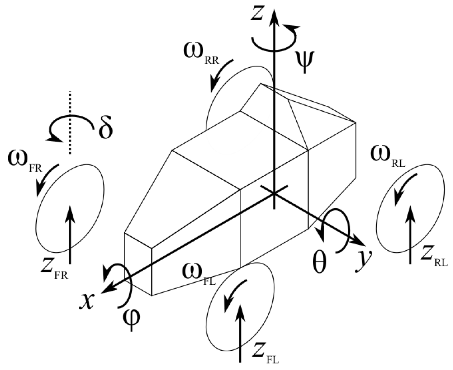
2.1. Vehicle Model

The vehicle was modeled according to a 14-degrees of freedom (dofs) model, as can be seen in Figure 2. The model accounted for:

• The three displacements of the vehicle center of mass;
• Three rotations about the vehicle center of mass (yaw, pitch, and roll);
• Four vertical displacements of unsprung masses; and
• Four wheel angular velocities about the hub axis.

2.2. Tire Model

The contact forces between tires and road were modeled according to an exponential tire model ([10]):

$$F_i=Z(A_{i}z{e}^{-b_{i}z}+B_i(1-e^{-b_{i}z}))\mathrm{sign}(z)$$

(1)

where Z is the vertical force, i is x or y for longitudinal and lateral forces, respectively, z is $\kappa$ (slippage) in the case of longitudinal forces, while it is $\alpha$ (slip angle) in the case of lateral forces. The coefficients were than computed according to the following equation:

$$\begin{array}{cc}\hfill A_x& =p_{x0}{e}^{p_{x1}{Z}^{\prime }}{e}^{p_{x2}\alpha }+p_{x3}\alpha ,\hfill \\ \hfill B_x& =(p_{x4}-p_{x5}{Z}^{\prime })(p_{x6}-p_{x7}\alpha ),\hfill \\ \hfill b_x& =p_{x8}{e}^{-p_{x9}*\alpha },\hfill \\ \hfill A_y& =p_{y0}{e}^{p_{y1}{Z}^{\prime }}{e}^{p_{y2}\kappa }+p_{y3}\kappa ,\hfill \\ \hfill B_y& =(p_{y4}-p_{y5}{Z}^{\prime })(p_{y6}-p_{y7}\kappa ),\hfill \\ \hfill b_y& =p_{y8}{e}^{-p_{y9}*\kappa },\hfill \end{array}$$

(2)

where $p_{i,j}$ are fixed coefficients and $Z^{\prime }$ is the normalized vertical load $Z^{\prime }=Z/1000$. In this way, the tire model accounted for combined slip effect. The resulting forces of the described model are reported in Figure 3. This model was used because of its simplicity in deriving various terms for vehicle equilibria computation. The computation of phase plots and controllability requires a smoothly analytic differentiable tire model which delivers reasonably simple terms in the Jacobian. Therefore, the model in [10] was used. The coefficients reported in the model were tuned by minimizing the root mean square error with respect to Pacejka tire model (For details on the comparison between the adapted model and the MF Tire model, the reader is referred to [10].). 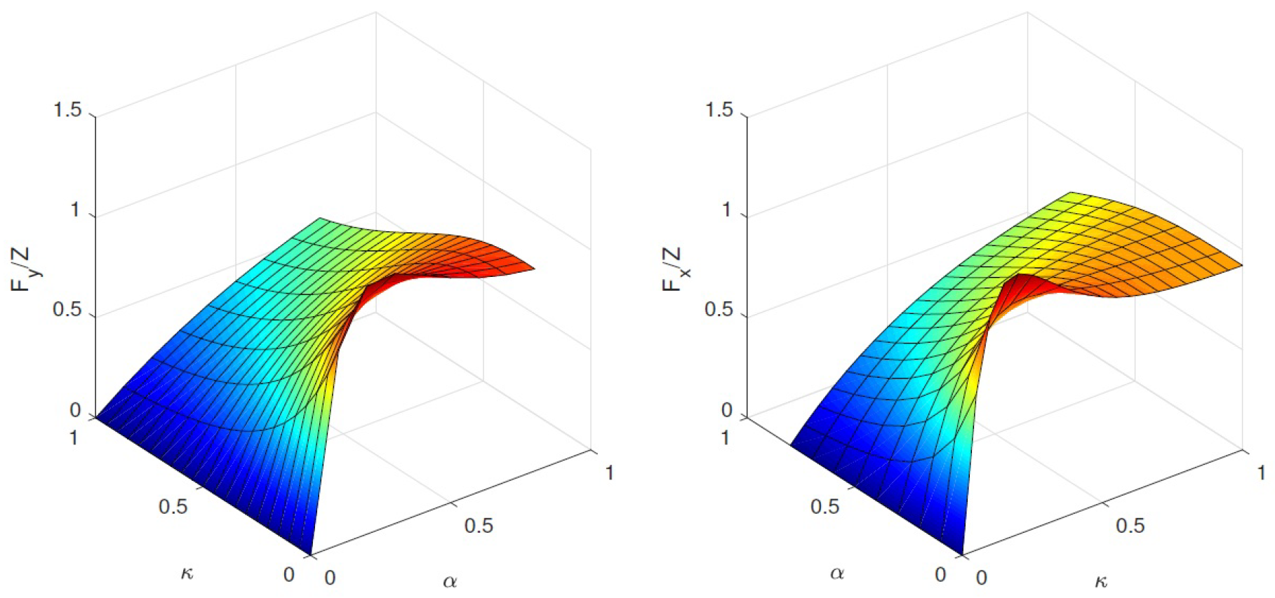Of course, other models could be used (e.g., [11,12]), but this one was preferred for its simplicity and its good representation of combined slip effect when compared with the Pacejka MF Tire model.

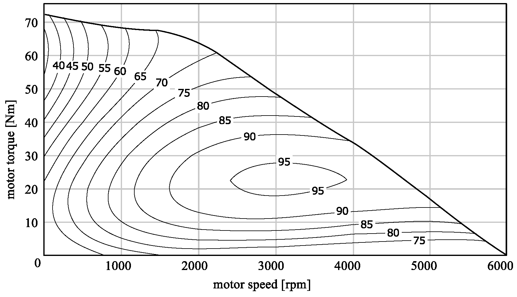
2.3. Electric Motor Model

The electric motors (EMs) were modeled accounting for the torque-speed characteristic, see Figure 4, giving upper and lower bounds to the available motor torque while the dynamics of the motor was accounted for by means of a first-order time lag transfer function

$$T{F}_{mot}=\frac{1}{{\tau }_{mot}s+1},$$

(3)

where ${\tau }_{mot}$ is the time constant, which also accounts for electronic drive dynamics. A rate limiter function was also included to model the electronic drive latency.

2.4. Driver Model

Since the drift equilibrium is an unstable one, the driver has the objectives of following the desired trajectory and keeping the vehicle stable. Acting on the demanded driving torque of the rear axle and on the steering wheel, the driver is able to maintain the vehicle in drift, following curves with different curvatures.

2.5. Close Loop Driver Model

The close-loop driver model indicated in Figure 5 was modeled as a proportional integral derivative (PID) controller that acts on the steering wheel angle ${\delta }_{SW}$ as a function of the curvature $\rho$ error (${\epsilon }_{\rho }={\rho }_{ref}-\rho$)

$${\delta }_{SW}=\sum _{i=1}^3{W}_i\left(k_{P,\delta }\epsilon +k_{I,\delta }\int \epsilon +k_{D,\delta }\dot{\epsilon }\right).$$

(4)

Similarly, the driver also acts on the throttle, changing the required driving torque $T_r$ as

$$T_r=\sum _{i=1}^3{W}_i{k}_{P,\gamma }\left(k_{P,\gamma }\epsilon +k_{I,\gamma }\int \epsilon +k_{D,\gamma }\dot{\epsilon }\right).$$

(5)

Such a control law on driving torque is dictated by the fact that, since we are in drift condition, we are in limit adherence conditions. This means that the friction is fully exploited by longitudinal and lateral forces (both present at the same time). Since the adherence is fully exploited, by increasing the driving torque (and so the longitudinal force), the lateral force on the drive axle (rear in this case) reduces. If the lateral force on the rear axle reduces, then the trajectory curvature increases. Conversely, when the driving force reduces, the lateral force of the rear axle increases and the curvature trajectory decreases.

The reference curvature was then evaluated at three different distances $l_i$ in order to simulate the preview capability of the driver. These distances are a function of vehicle speed

$$l_i=v{t}_i,$$

(6)

where $t_i$ are the driver response times. To each preview length was associated a weight $W_i$, which was 0.5 for $l_1$, 0.35 for $l_2$, and 0.15 for $l_3$. In this way, more importance was given to closer points.

The reference curvature ${\rho }_{\mathrm{ref},i}$ is given by the following expression:

$${\rho }_{\mathrm{ref},i}=\frac{2sin(0.5({\psi }_{\mathrm{ref}}-\psi -\beta ))}{L_{\mathrm{ref},i}},$$

(7)

where $L_i$ is the distance between reference point on the trajectory and the cog position. It was assumed that the vehicle was close to the reference trajectory.

By changing the values of PIDs gains, it is possible to simulate different driver behavior: highly skilled (higher gains, more prompt PID), low-skilled (lower gains, less-prompt PID).

This close-loop driver was used to follow the reference curvature while the vehicle was in drift condition. In order to achieve the drift condition, an open-loop driver is necessary.

2.6. Open-Loop Steer Actuation

As underlined previously, the previous driver model (i.e., closed loop) can only work once the vehicle is already in drift condition. Thus, it was necessary to implement an open-loop maneuver that allows entering that region of behavior and, finally, another one to exit from drift equilibrium and leave the driver to go for a stable condition (e.g., following a straight path) or to approach another drift curve. These maneuvers were developed by imposing a certain time history of the driver inputs (i.e., steer angle ${\delta }_{SW}$ and wheel torque $T_i$) based on the sequence of actions that an expert driver would perform in those kinds of conditions.

Looking at Figure 6, the beginning of the drift maneuver was thus performed according to the following sequence of steer and throttle/brake open-loop actuation:

0

Straight forward driving;

1a

Apply a strong braking torque at the rear wheels (e.g., a handbrake actuation);

1b

Apply a strong steering stroke in the direction of the turn;

2a

Cancel braking torque and accelerate;

2b

Countersteer;

3

Switch to feedback driver model in drift condition.

This procedure would replicate the human driver behavior that starts the drift maneuver in feed forward without accounting for the straight trajectory and then starts controlling the drift in a feedback manner.

2.7. Vehicle Equilibria and Input Effects

Before presenting the newly designed control strategy, it is interesting to better understand the vehicle lateral dynamics and its equilibrium points and the effect of different inputs on the vehicle dynamics. This can be done considering the handling diagram and the phase portrait ([13]).

More specifically, it is interesting to understand if and how the torque-vectoring can influence the vehicle dynamics. This was examined by using two tools typical of control design: the phase portrait of the system and the controllability matrix. In the following, the phase portrait of the vehicle is analyzed to show how the controller can change the vehicle behavior in the phase plane. Then, using the linearized system matrices, the torque-vectoring authority on the vehicle dynamics is analyzed and compared to the other inputs (i.e., the driver’s inputs: steering wheel and accelerator pedal).

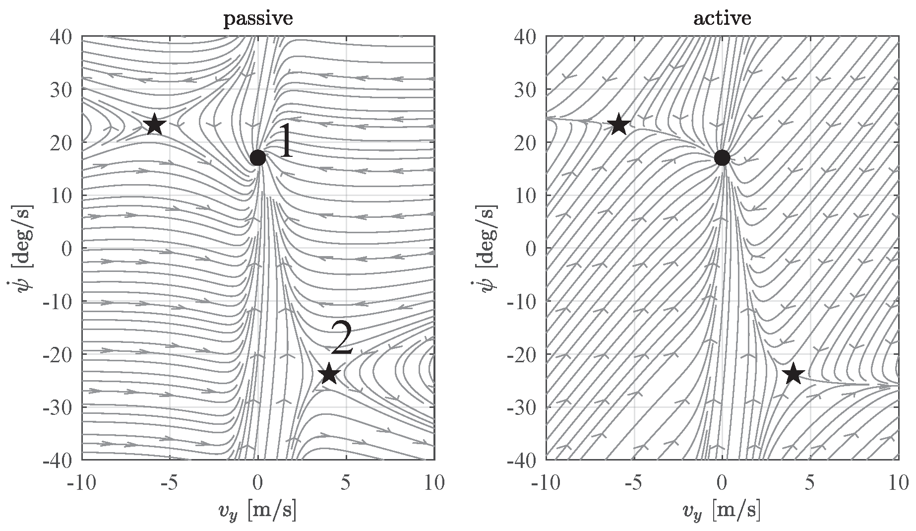
2.7.1. Phase Portrait

The phase portrait and the study of vehicle equilibria was performed according to the following nonlinear single-track vehicle model ([14]) under the following hypotheses:

• Constant forward speed $v_x$.
• The resultant of the contact forces acting on each axle are applied in the center of the axle itself.
• Lateral load transfers are accounted for by considering steady-state axle characteristics.
• The longitudinal slip $\kappa$ of the rear axle is accounted for as described in the following, while the front axle has no driving/braking force.
• Small steering angles are considered.

The equation of motion thus read:

$$\{\begin{array}{c}m{\dot{v}}_y=-m{v}_x\dot{\psi }+F_{y,f}cos\delta +F_{y,r},\hfill \\ J\ddot{\psi }=F_{y,f}cos\delta l_f-F_{y,r}{l}_r+M_z,\hfill \end{array}$$

(8)

where $M_z$ is the yaw moment applied by the torque-vectoring control. $F_y$ are the contact forces modeled according to the previously presented tire model, see Equations (1) and (2), referring to the front and rear axles, respectively. The combined slip effect was accounted for by computing the mean slip $\kappa$ of the rear wheels by inverting the longitudinal force expression. The value of mean rear longitudinal force $F_{x,r}$ was obtained from the following equation:

$$m{a}_x=F_{x,r}(\kappa )-F_{res},$$

(9)

which represents the vehicle longitudinal dynamic equilibrium in which $a_x$ is imposed to be equal to 0. $F_{res}$ is the total resistance force which accounts for rolling resistance and aerodynamic drag force.

Equation (8) can thus be written in short form as

$$\dot{\mathit{z}}=\mathit{f}(\mathit{z},\mathit{u}),$$

(10)

where $\mathit{z}$ is the state vector

$$\mathit{z}={\{v_y\dot{\psi }\}}^T,$$

(11)

while $\mathit{u}$ is the inputs vector

$$\mathit{u}={\{v_x\delta M_z\}}^T.$$

(12)

The fixed points could be found by imposing

$$\mathit{f}(\mathit{z},\mathit{u})=\mathbf{0}.$$

(13)

Figure 7 reports the phase portraits of the passive (left figure) and active (right figure) vehicles obtained with the model in (8). The active vehicle had the control law described in the following paragraphs, which anticipate the results in the phase plot.

In the phase portraits, the equilibria are marked with different markers according to the nature of the node: • for stable nodes, ⋆ for saddle nodes, and ∘ for unstable nodes.

As can be noticed, the controller did not affect the position or stability of nodes, but it did affect the behavior of the system in the neighborhood of the nodes. In particular, the controller increased the damping of the system with respect to yaw rate, making the yaw rate converge more quickly to the equilibrium value. This results in helping the driver, who would be better able to control the drifting maneuver.

2.7.2. Input Effect on Vehicle Dynamics

Considering the model Equation (8), it is also interesting to understand the effects of different inputs on the vehicle dynamics. In order to compare the effect of the rear drive force and steering angle as inputs, as well as the yaw moment due to torque-vectoring control at different operating conditions, it is possible to evaluate their ability to influence the vehicle state derivatives around those operating conditions ([13]). Towards this end, the state space representation of the linearized vehicle dynamics was examined around equilibria corresponding to different kinds of operating conditions. Linearizing the following set of Equation (8) and explicating the sideslip angle $\beta$:

$$\{\begin{array}{c}\dot{\beta }=\frac{1}{mV}\left(F_{yf}cos\delta +F_{y,r}\right)-\dot{\psi },\hfill \\ \ddot{\psi }=\frac{1}{J}\left(F_{y,f}cos\delta l_f-F_{y,r}{l}_r\right)+\frac{M_z}{J}.\hfill \end{array}$$

(14)

The combined slip effect is accounted for thanks to the previously presented tire model and by computing the mean slip $\kappa$ of the rear wheels by inverting the longitudinal force expression. The value of mean rear longitudinal force $F_{x,r}$ is obtained from the following equation:

$$m{a}_x=F_{x,r}(\kappa )-F_{res},$$

(15)

which represents the vehicle longitudinal dynamic equilibrium in which $a_x$ is imposed to be equal to 0. $F_{res}$ is the total resistance force which accounts for rolling resistance and aerodynamic drag force.

The linearized system, about one of the equilibrium points, takes the form

$$\partial \dot{x}=[A]\partial x+[B]\partial u,$$

(16)

where x is the state vector

$$\partial x=\left\{\partial \beta \partial \dot{\psi }\right\}$$

(17)

and $[A]$ the plant state matrix

$$[A]=\left[\begin{array}{cc}\frac{\partial \dot{\beta }}{\partial v_y}& \frac{\partial \dot{\beta }}{\partial \dot{\psi }}\\ \frac{\partial \ddot{\psi }}{\partial v_y}& \frac{\partial \ddot{\psi }}{\partial \dot{\psi }}\end{array}\right]=\left[\begin{array}{cc}{a}_{11}& a_{12}\\ a_{21}& a_{22}\end{array}\right].$$

(18)

Since the inputs to the system, i.e., steering angle $\delta$, accelerator pedal $\gamma$, and torque-vectoring yaw moment $M_z$, are of different nature and thus of different orders of magnitude:

$$\begin{array}{ccc}\delta & \left(\mathrm{rad}\right)& -0.17<\delta <0.17,\\ \gamma & \left(\right)& 0<\gamma <1,\\ M_z& \left(\mathrm{Nm}\right)& -300<M_z<300,\end{array}$$

(The considered value of $M_z$ was 50% of the maximum exploitable yaw moment when considering the maximum longitudinal force that can be applied on the inner rear wheel. This value was computed considering also the load transfer in a turn with maximum lateral acceleration ($\mathsf{\mu }$g)) it is more convenient to study the perturbation effects due to the contact forces which are directly affected by the driver’s and TV inputs:

• $\partial F_{yf}$—front lateral force, which is directly affected by the steering angle;
• $\partial F_{xr}$—rear longitudinal force, which is directly controlled by gas pedal $\gamma$;
• $\partial \Delta F_{xr}$—the difference in left and right rear longitudinal forces induced by yaw moment $M_z$.

In this way, the input matrix $[B]$ can be written as

$$[B]=\left[\begin{array}{ccc}\frac{\partial \dot{\beta }}{\partial F_{yf}}& \frac{\partial \dot{\beta }}{\partial F_{xr}}& \frac{\partial \dot{\beta }}{\partial \Delta F_{xr}}\\ \frac{\partial \ddot{\psi }}{\partial F_{yf}}& \frac{\partial \ddot{\psi }}{\partial F_{xr}}& \frac{\partial \ddot{\psi }}{\partial \Delta F_{xr}}\end{array}\right]=\left[\begin{array}{ccc}{b}_{11}& b_{12}& b_{13}\\ b_{21}& b_{22}& b_{23}\end{array}\right].$$

(19)

Considering the different equilibrium points of the vehicle under different driving conditions, it is thus possible to evaluate the influence of the inputs upon the sideslip angle and yaw rate dynamics. Note that $F_{xr}$ does not appear explicitly inside the equations, but it does affect the rear cornering force due to the coupling effect in combined slip condition. The terms $b_{12}$ and $b_{22}$ of matrix $[B]$ are thus different from zero when the coupling between longitudinal and lateral forces becomes evident (i.e., in the case of high values of slip and slip angles). Considering a constant speed $v_x$ of 8 m/s, three different driving conditions were analyzed: straight driving, typical cornering, and drift cornering. The computed matrices are reported in

Table 2. Input effects on vehicle dynamics for three driving conditions at 8 m/s forward speed. The reported values were multiplied by a factor ${10}^3$.

	Straight Driving	Typical Cornering	Drift Cornering
$[B]=·$	$\left[\begin{array}{ccc}0.402& 0& 0\\ 3.740& 0& 6.380\end{array}\right]$	$\left[\begin{array}{ccc}0.402& 0.008& 0\\ 3.740& -0.091& 6.38\end{array}\right]$	$\left[\begin{array}{ccc}0.402& 0.268& 0\\ 3.740& 3.090& 6.38\end{array}\right]$

. Specifically, the matrices were respectively obtained by linearizing the system in the neighborhood of three equilibrium points:

• Straight driving: $\delta =0$, $\beta =0$, $\dot{\psi }=0$;
• Typical cornering: point 1 in Figure 7 left;
• Drift cornering: point 2 in Figure 7 left.

Upon analyzing the data reported in the table, the following considerations can be drawn:

• In straight driving, the gas pedal (i.e., $F_{xr}$) did not affect the sideslip angle or the yaw rate dynamics ($b_{12}=b_{22}=0$). The steering angle and the torque-vectoring moment instead had comparable effects on yaw rate while the effect on sideslip angle was null for TV. This was because $\Delta F_{xr}$ had a higher-order contribution to the combined slip effect of the axle since the total driving force was not affected by $M_z$.
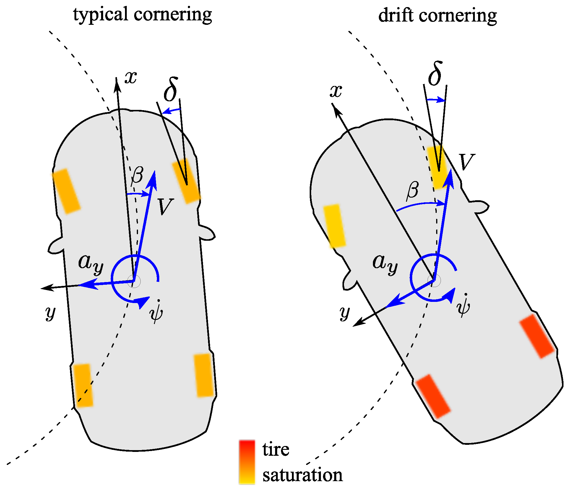
• In typical cornering, the effects were similar to those of straight driving but a small coupling effect of gas pedal was noticed on both sideslip angle and yaw rate. However, these effects were two orders of magnitude smaller than steering wheel effects. Again, the effect of TV on yaw rate was comparable to that of steering wheel.
• In drift cornering, the effects of the gas pedal became higher and comparable with those of steering wheel and TV. Again, the effects of steering wheel and TV on yaw rate were comparable.

In conclusion, the steering wheel had a strong influence on vehicle lateral dynamics in all driving conditions. The gas pedal could affect the vehicle lateral dynamics in cornering, but its effects were comparable to steering wheel only in drift cornering conditions. Torque vectoring was effective in controlling yaw rate in all driving conditions. Since the main idea of the paper was to design an assisting system for the driver, it is preferable to use TV instead of modifying the driver’s inputs.

TV has no generalized force on sideslip angle ($b_{13}=0$). Nevertheless, the torque-vectoring input can be used to control the sideslip angle thanks to the coupling between the system equations, thus resulting in a non-collocated control. Looking at the system controllability matrix $[R]$, considering only the column of $[B]$ related to $M_z$ ($[B_3]={[0b_{23}]}^T$), it reads

$$[R]=\left[\begin{array}{cc}[B_3]& [A][B_3]\end{array}\right]=\left[\begin{array}{cc}0& a_{12}{b}_{13}\\ b_{13}& a_{22}{b}_{13}\end{array}\right],$$

(20)

whose determinant is

$$det[R]=a_{12}{b}_{13}^2.$$

(21)

If the rank of matrix $[R]$ is full, then the system is controllable ([15]), which means that the system is controllable if $a_{12}\ne 0$. That is, $C_f{l}_{f}cos\delta \ne C_r{l}_r$ ($C_f$ and $C_r$ are front and rear cornering force slopes in the $F_y$–$\alpha$ curve, i.e., $\partial F_y/\partial \alpha$). This condition is generally difficult to obtain, such as with a neutral vehicle with no driving forces or with equal front/rear distribution of driving forces. Moreover, this condition is true only in steady-state condition, while it never occurs around the equilibrium point (i.e., in transient conditions). The designed controller, as better explained in the following, acts only during transients not at steady-state.

As mentioned earlier, this means that when the vehicle is not neutral and driving forces are applied due to torque-vectoring and power-slide, $a_{12}\ne 0$. Thus, the system is controllable having matrix R full rank ([15]).

3. Drift Torque-Vectoring Active Control

Based on the previous study, thanks to torque-vectoring it is possible to design an advanced driver-assistance system (ADAS) which helps the driver to control the vehicle during drift without modifying the driver’s inputs (i.e., steering wheel and accelerator/brake pedals).

The controller was designed in order to leave the driver free to define vehicle attitude. The controller generates a yaw moment according to the following equation:

$$M_z=k_{\mathrm{Y}}·I_{\mathrm{Y}},$$

(22)

where $k_{\mathrm{Y}}$ is the controller gain and $I_{\mathrm{Y}}$ is the yaw index expressed as

$$I_{\mathrm{Y}}=\frac{a_y}{v_x}-\dot{\psi },$$

(23)

where $a_y$ is the vehicle lateral acceleration, $v_x$ is the vehicle forward velocity, and $\dot{\psi }$ is the yaw rate.

Controlling $I_Y$ means to control the time derivative of lateral velocity $v_y$. Considering that the lateral acceleration $a_y$ can be written as

$$a_y={\dot{v}}_y+v_x\dot{\psi },$$

(24)

rearranging the equation, we obtain

$$\frac{{\dot{v}}_y}{v_x}=\frac{a_y}{v_x}-\dot{\psi },$$

(25)

which means that the controller generates a yaw moment that prevents lateral velocity from excessive increase. This makes the vehicle more straight-forward for the driver, who can control the vehicle more smoothly.

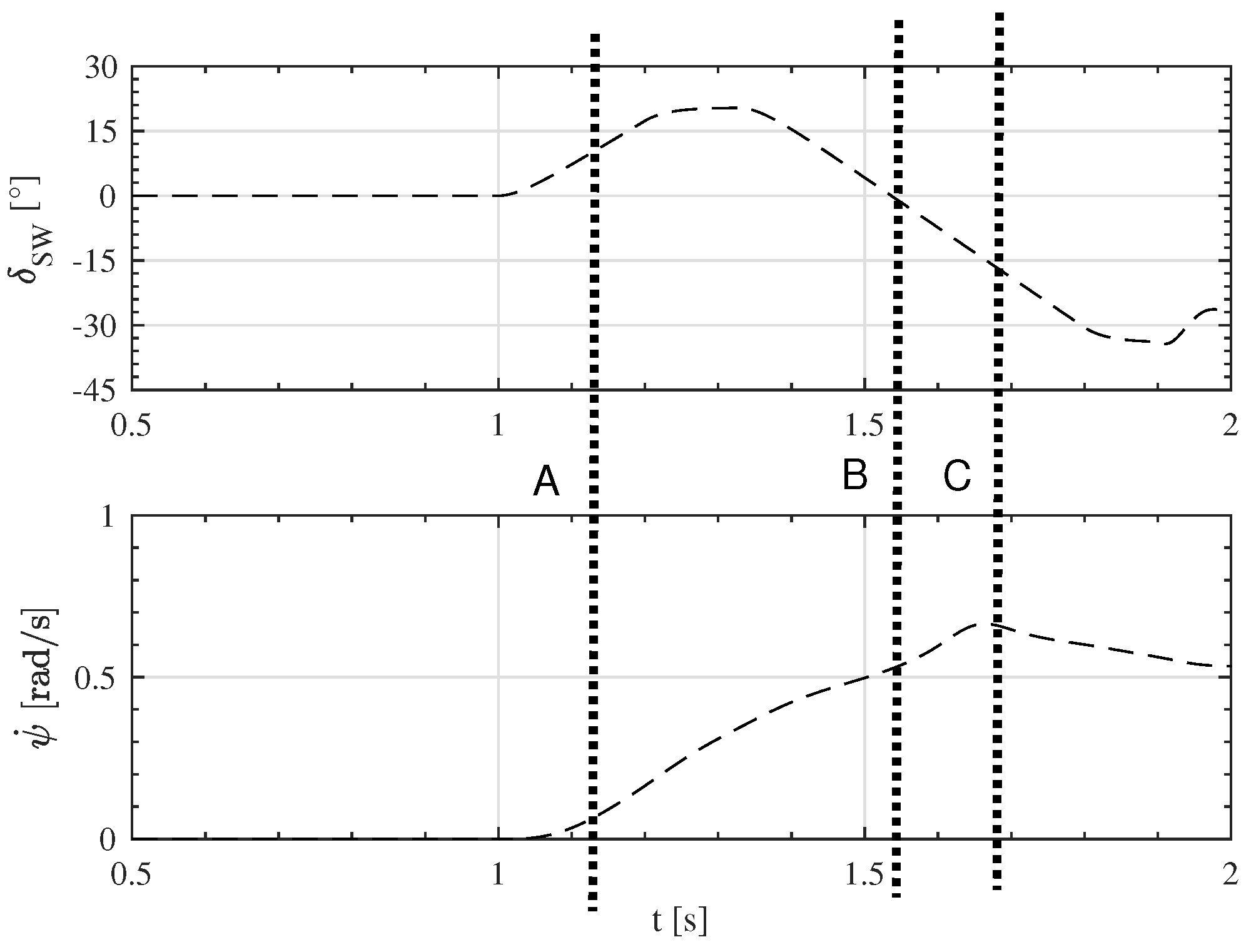
3.1. Control Activation Conditions

The controller must be activated only when the drift condition is detected, otherwise its intervention could conflict with driver’s will. The autonomous activation procedure is reported here and explained thanks to Figure 8, which reports the yaw rate and the steering wheel time history at the beginning of the drift maneuver.

The activation is based on a set of cascading conditions that must be verified so that the control turns on. Below we list a series of conditions that allow the control to be activated:

Condition A 

identifies the entrance in a turn by looking at the yaw rate of the vehicle. A small threshold is used to avoid intervention due to measurement noise. Condition A reads:

$$\left|\dot{\psi }\right|>{\dot{\psi }}_{lim}.$$

(26)

Condition B 

identifies the beginning of the counter-steering action by the driver. Condition B thus reads:

$$sgn(\delta )\ne sgn(\dot{\psi }).$$

(27)

Condition C 

identifies the beginning of the drift due to the permanence of the steering wheel in counter-steer condition:

$$\overline{\delta }·sgn(\overline{\dot{\psi }})<0,$$

(28)

where for robustness both $\delta$ and $\dot{\psi }$ are accounted for by means of their average value evaluated ($\overline{\delta }$ and $\overline{\dot{\psi }}$) with a moving average window of 0.5 s.

3.2. Control Deactivation Conditions

The controller is then deactivated when the drift maneuver is ended by the driver. This condition is identified by a reduction, or a change in sign if the vehicle oscillates, of the yaw rate

$$\left|\dot{\psi }\right|<{\dot{\psi }}_{lim}$$

(29)

or

$${\dot{\psi }}_k·{\dot{\psi }}_{k-1}<0.$$

(30)

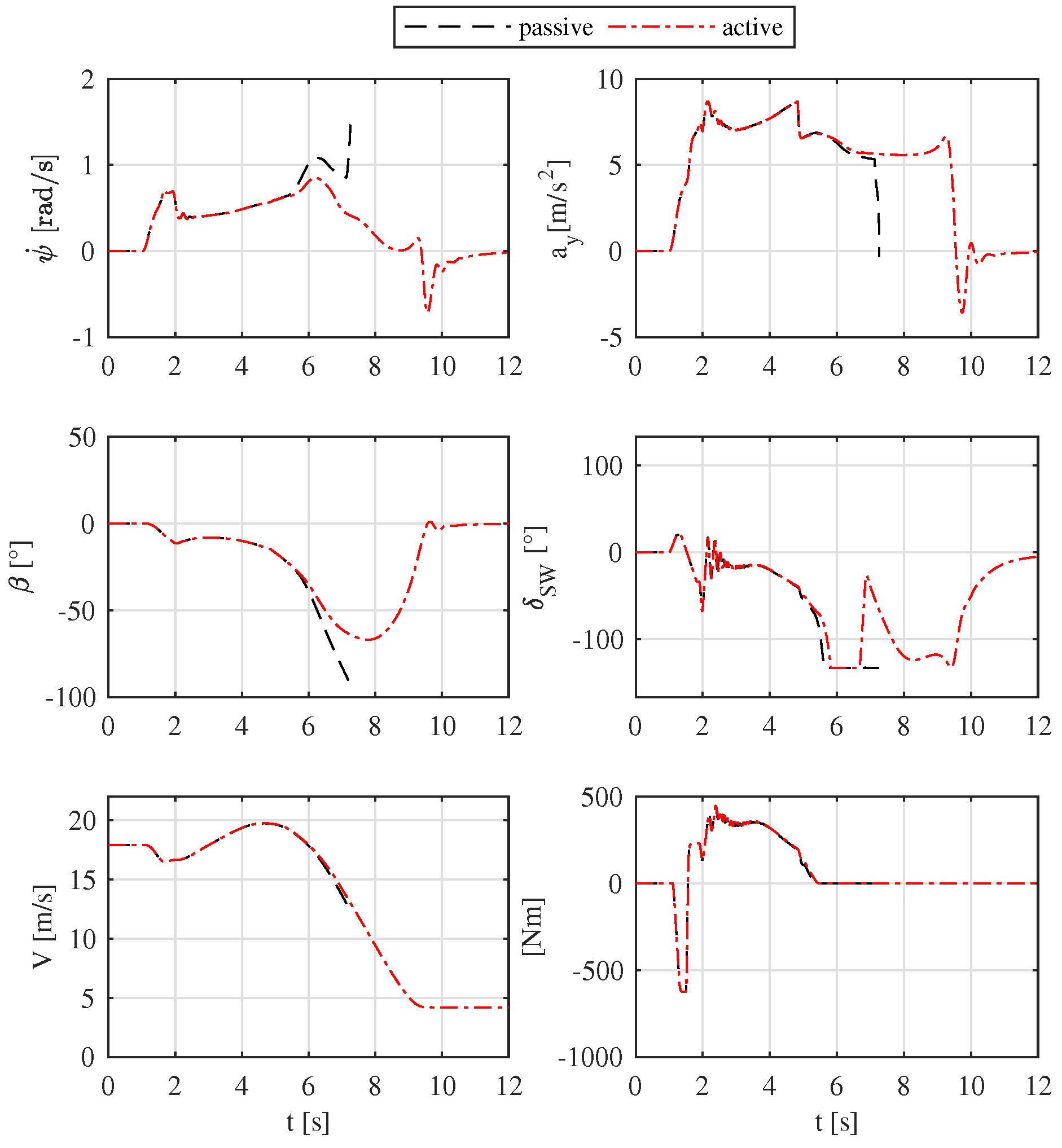
4. Simulation Results

The control strategy was tested according to the following maneuver, which consists of a constant-speed U-turn on different adherence road surfaces and for different drivers. The two modeled drivers were a highly skilled driver and a low-skilled driver. The difference in the two drivers was in the value of PID gains, as described previously.

The vehicle started from straight line condition with velocity $V=18$ m/s. The turn had a radius R of 38 m. The following simulation results report the following quantities related to vehicle dynamics behavior:

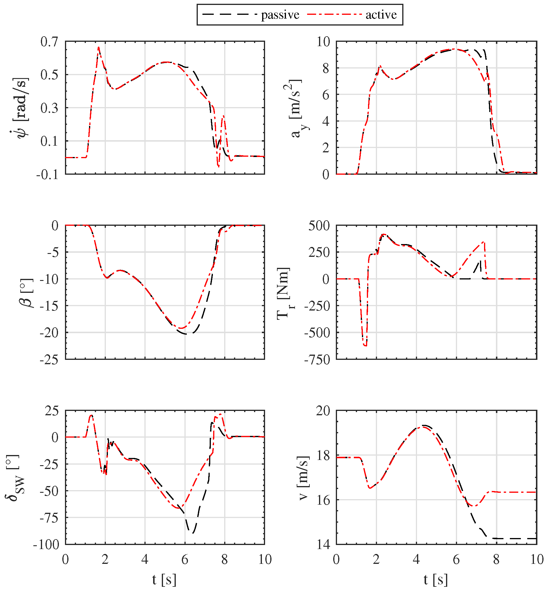
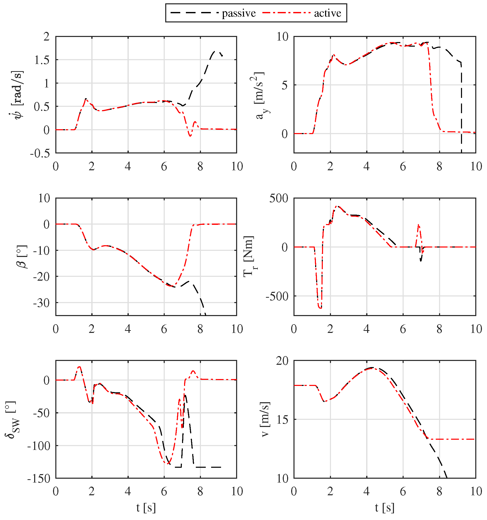
• Vehicle yaw rate $\dot{\psi }$;
• Vehicle lateral acceleration $a_y$;
• Vehicle sideslip angle $\beta$;
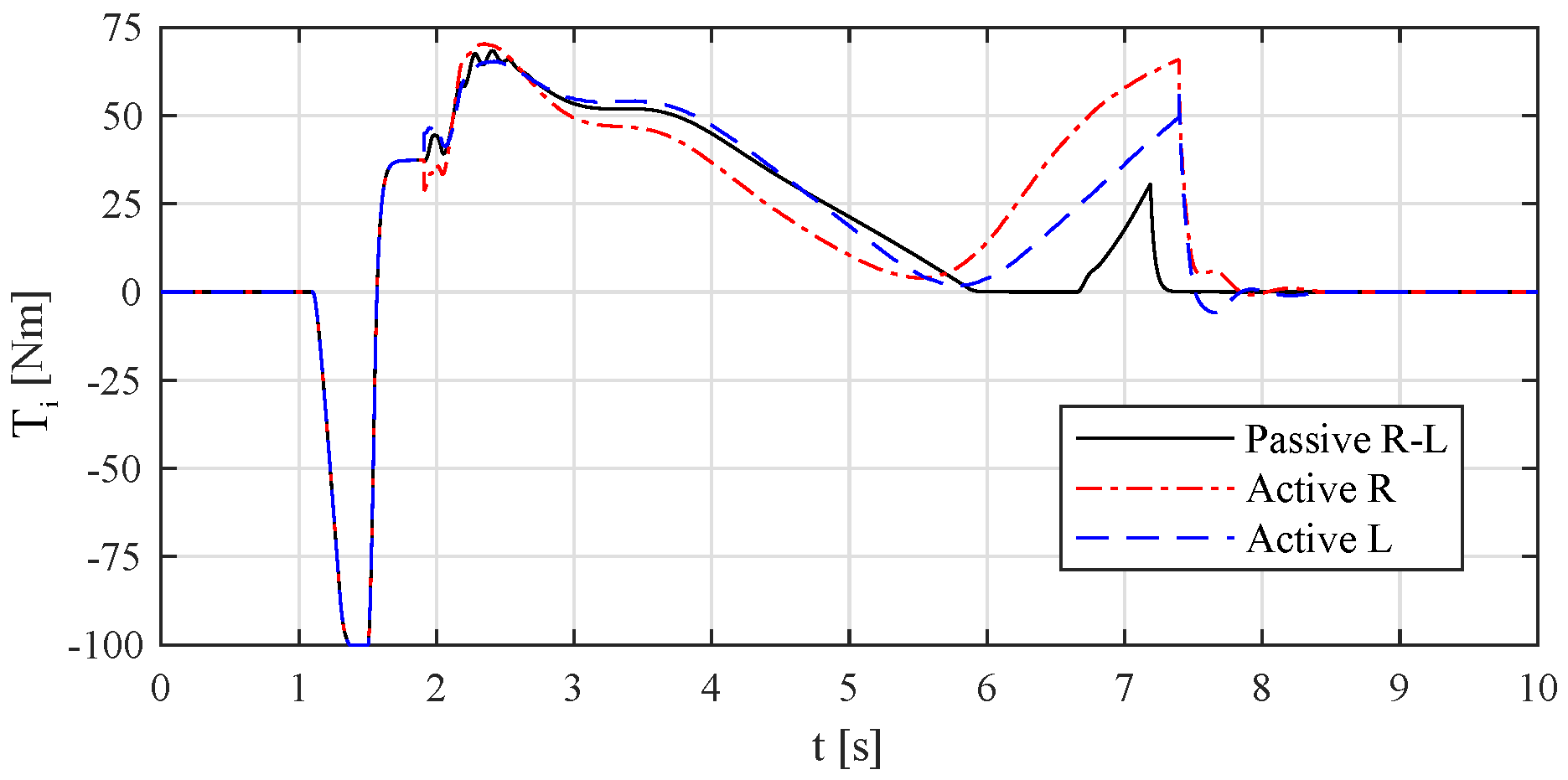
• Driver required driving torque $T_r$;
• Steering wheel angle ${\delta }_{SW}$;
• Vehicle speed V.

The sign convention is consistent with Figure 2.

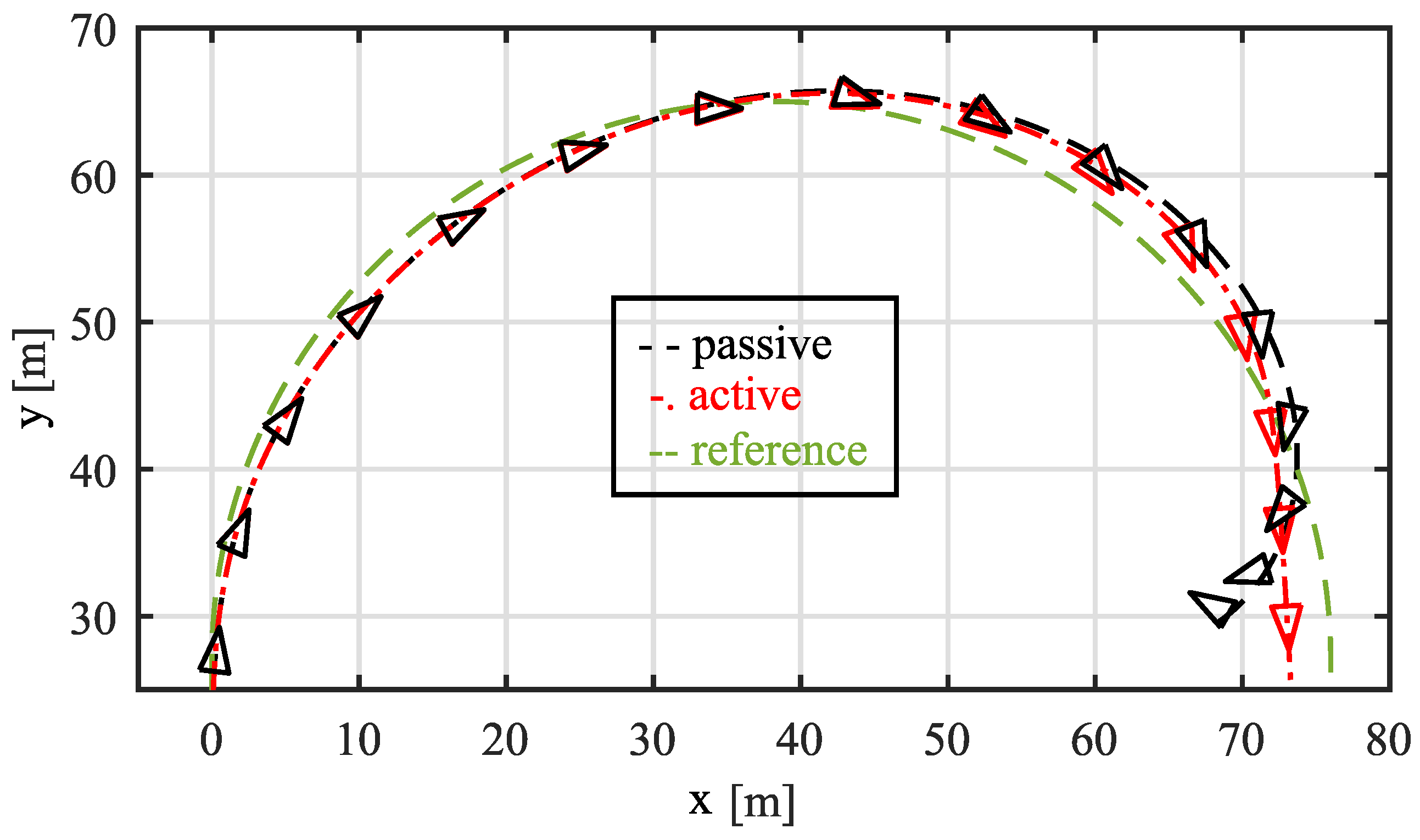
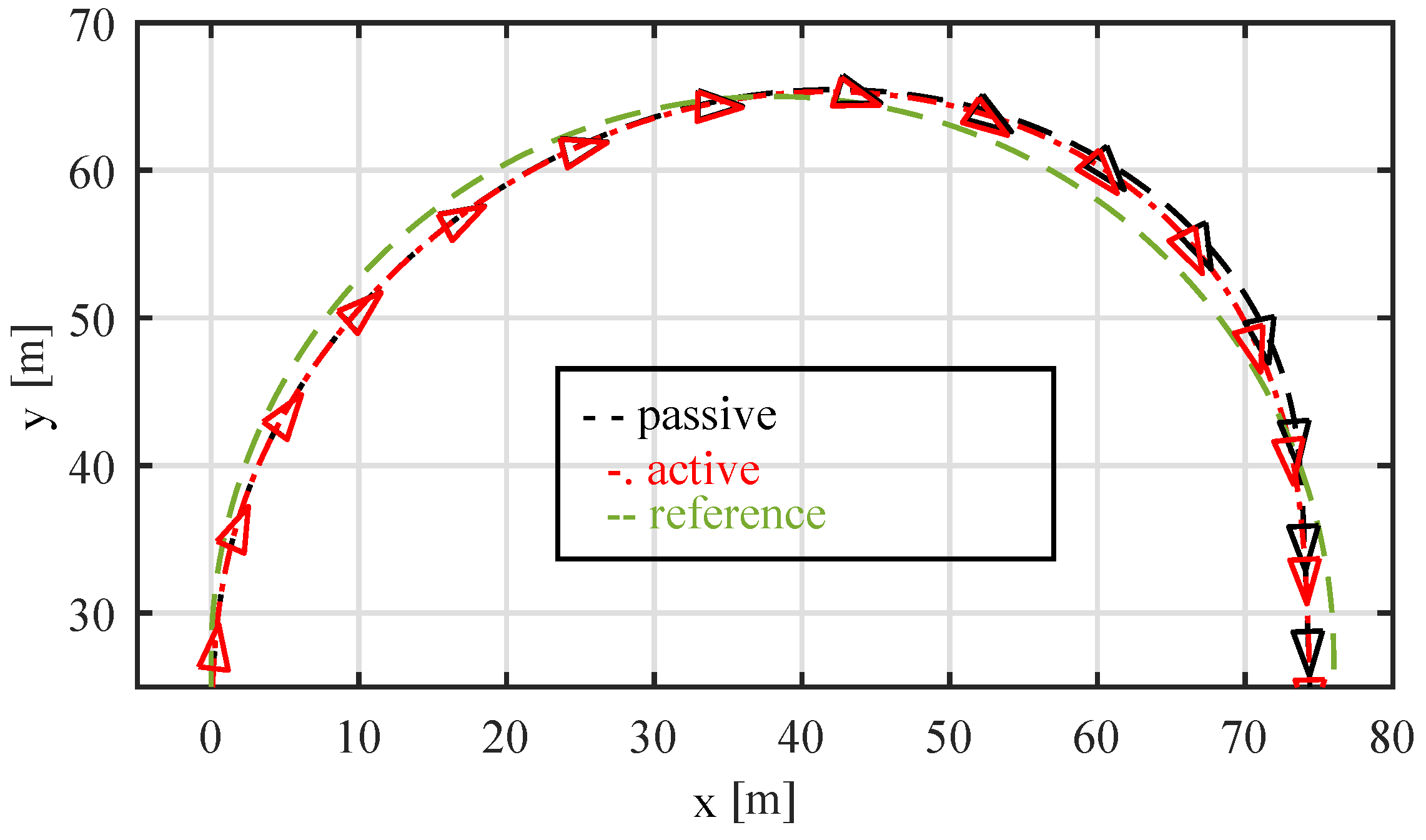
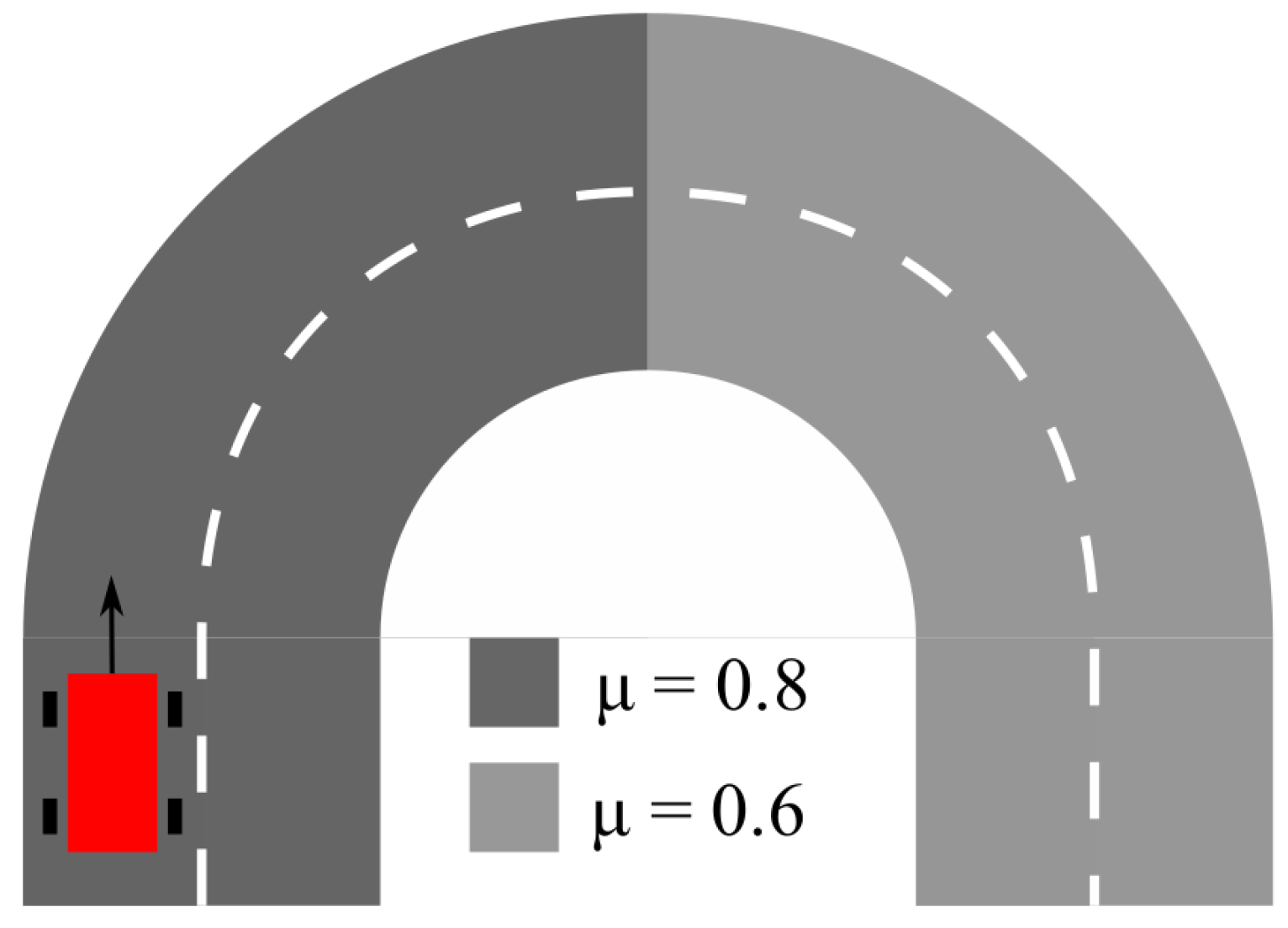
4.1. U-Turn—Highly Skilled Driver

The maneuver described here is a U-turn with constant radius in which the performances of the passive vehicle is compared to the active one, both driven by the same highly skilled driver. Figure 9 reports the trajectory of the passive and active vehicle cogs, respectively. The triangle in the figure reports the direction of the vehicle x-axis starting from the vehicle cog. Figure 10 reports instead the principal dynamics and Figure 11 reports the torques applied by the controller. The first 2 s of simulations were imposed in feed-forward by the driver in order to start the drift maneuver.

As can be noticed from Figure 10, the driver could perform the maneuver easily when the control was active. This can be seen by the steering wheel angle ${\delta }_{SW}$ that for the passive vehicle had a peak value, in modulus, of about 90 degrees, while for the active vehicle it was lower than 70 degrees. Additionally, the dynamics of the car improved: the sideslip angle had a smaller peak value. Finally, the final speed of the vehicle v was higher for the active vehicle by about 2 m/s (7.2 km/h).

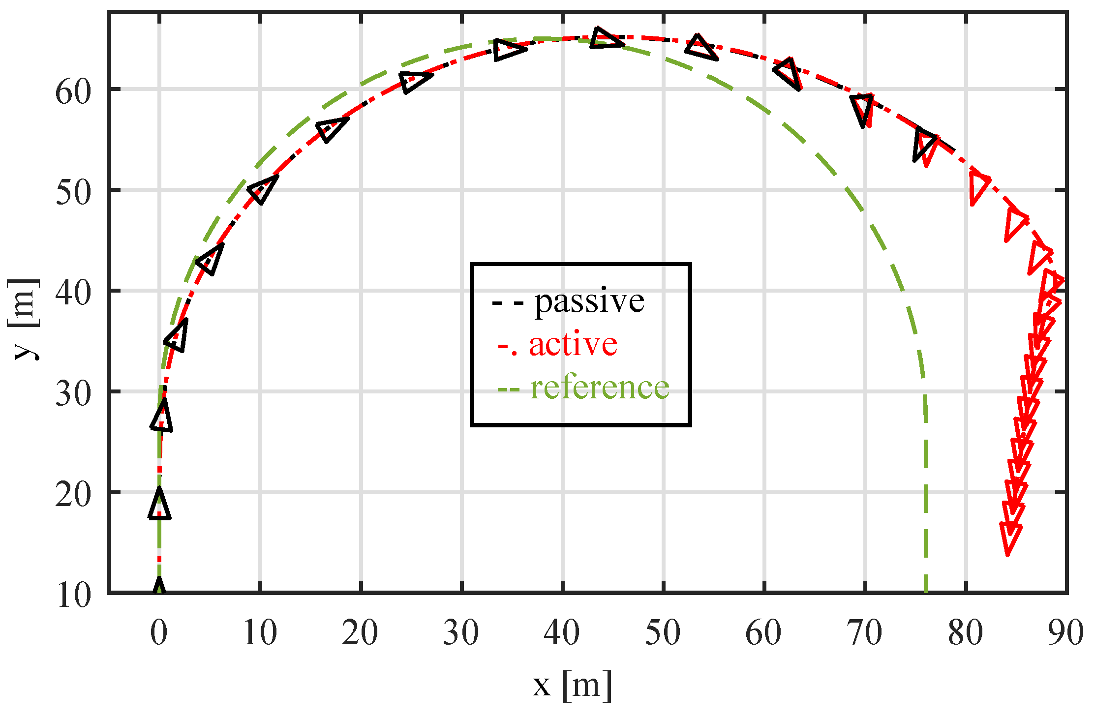
4.2. U-Turn—Low-Skilled Driver

The previously presented maneuver was repeated, changing the promptness of the driver (i.e., the gains of the driver were reduced). Figure 12 shows the trajectory resulting from the simulation while Figure 13 shows the vehicle dynamics quantities.

In this case, the driver was not able to maintain the stability of the passive vehicle that underwent a tail spin. Instead, in the case of the active vehicle, the driver did not lose the vehicle and could complete the maneuver. However, the error in following the trajectory was high.

4.3. U-Turn—$\mu$ Jump

In order to further test the effectiveness of the controller, the U-turn maneuver was also simulated with a friction jump in the middle of the turn, as reported in Figure 14. The driver was the highly skilled driver of the first presented maneuver.

The simulation results (Figure 15 and Figure 16) show that the driver without any controls was not capable of keeping the vehicle stable when a sudden drop of the friction coefficient happened. Since the friction decreased, the driver could not sustain the required curvature with the actual velocity, so the vehicle tended to find a new equilibrium position with a smaller curvature and velocity value. This happened for both passive and active vehicles. However, Figure 15 shows an increase of the curvature for the passive vehicle when the friction dropped (t = 5 s), so the vehicle tended to go into a tail spin. The driver tried to counteract with the steering angle ${\delta }_{SW}$ and the rear motors $T_r$, but it was not enough and both control inputs saturated. So, the driver did not manage to stabilize the drift and the vehicle went into tail spin.

The active vehicle, instead, made the driver able to complete the turn thanks to a smart distribution of the rear motors’ torques that aimed to go against the variation of the sideslip angle. However, the driver could not follow the reference trajectory properly.

5. Conclusions

The paper presents a control strategy that can help the driver in high-sideslip maneuvers, namely, in drift condition. The control inputs are the torques on the rear wheels, which are independent thanks to electric motors. A torque-vectoring-based control strategy is then set up and tested in Matlab-Simulink simulation environments.

Note that the developed control strategy relies only on measured quantities (i.e., lateral acceleration, yaw rate, and wheel speed). This makes the controller robust and independent from state estimators.

Results demonstrated that it was possible to help the stabilization of drift cornering, without making use of the driver’s inputs but thanks to a smart distribution of rear motor torques. This type of control allows a collaboration between the driver and the control logic, so that the control does not replace the driver entirely. Especially, it is shown that the presented control allows even less skilled drivers to keep the vehicle stable in drift cornering, which would be very difficult without it.

References

- Vignati, M.; Sabbioni, E.; Tarsitano, D.; Cheli, F. Electric powertrain layouts analysis for controlling vehicle lateral dynamics with torque-vectoring. In Proceedings of the 2017 International Conference of Electrical and Electronic Technologies for Automotive, Torino, Italy, 15–16 June 2017; pp. 1–5. [Google Scholar] [CrossRef]
- Dizqah, A.M.; Lenzo, B.; Sorniotti, A.; Gruber, P.; Fallah, S.; De Smet, J. A Fast and Parametric Torque Distribution Strategy for Four-Wheel-Drive Energy-Efficient Electric Vehicles. IEEE Trans. Ind. Electron. 2016, 63, 4367–4376. [Google Scholar] [CrossRef]
- Hoffman, R.C.; Stein, J.L.; Louca, L.S.; Huh, K. Using the Milliken Moment Method and dynamic simulation to evaluate vehicle stability and controllability. Int. J. Veh. Des. 2008, 48, 132. [Google Scholar] [CrossRef]
- Edelmann, J.; Plöchl, M. Analysis of controllability of automobiles at steady-state cornering considering different drive concepts. In Dynamics of Vehicles on Roads and Tracks; CRC Press: London, UK, 2018. [Google Scholar]
- Velenis, E.; Frazzoli, E.; Tsiotras, P. Steady-state cornering equilibria and stabilisation for a vehicle during extreme operating conditions. Int. J. Veh. Auton. Syst. 2010, 8, 217–241. [Google Scholar] [CrossRef]
- Edelmann, J.; Plöchl, M. Handling characteristics and stability of the steady-state powerslide motion of an automobile. Regul. Chaotic Dyn. 2009, 14, 682–692. [Google Scholar] [CrossRef]
- Velenis, E.; Katzourakis, D.; Frazzoli, E.; Tsiotras, P.; Happee, R. Steady-state drifting stabilization of RWD vehicles. Control Eng. Pract. 2011, 19, 1363–1376. [Google Scholar] [CrossRef]
- Werling, M.; Reinisch, P.; Gröll, L. Robust power-slide control for a production vehicle. Int. J. Veh. Auton. Syst. 2015, 13, 27. [Google Scholar] [CrossRef]
- Nakano, H.; Okayama, K.; Kinugawa, J.; Kosuge, K. Control of an electric vehicle with a large sideslip angle using driving forces of four independently-driven wheels and steer angle of front wheels. In Proceedings of the 2014 IEEE/ASME International Conference on Advanced Intelligent Mechatronics, Besancon, France, 8–11 July 2014; pp. 1073–1078. [Google Scholar] [CrossRef]
- Best, M.C. Exploring Assumptions and Requirements for Continuous Modification of Vehicle Handling Using Nonlinear Optimal Control and a New Exponential Tyre Model; Loughborough University: Loughborough, UK, 2010; pp. 79–84. [Google Scholar]
- Hindiyeh, R.Y.; Gerdes, J.C. Design of a Dynamic Surface Controller for Vehicle Sideslip Angle During Autonomous Drifting. IFAC Proc. Vol. 2010, 43, 560–565. [Google Scholar] [CrossRef]
- Bobier-Tiu, C.G.; Beal, C.E.; Kegelman, J.C.; Hindiyeh, R.Y.; Gerdes, J.C. Vehicle control synthesis using phase portraits of planar dynamics. Veh. Syst. Dyn. 2018, 3114, 1–20. [Google Scholar] [CrossRef]
- Hindiyeh, R.Y.; Gerdes, J.C. Equilibrium Analysis of Drifting Vehicles for Control Design. In Proceedings of the ASME 2009 Dynamic Systems and Control Conference, Hollywood, CA, USA, 12–14 October 2009; Volume 1, pp. 181–188. [Google Scholar] [CrossRef]
- Rossa, F.; Gobbi, M.; Mastinu, G.; Piccardi, C.; Previati, G. Bifurcation analysis of a car and driver model. Veh. Syst. Dyn. 2014, 52, 142–156. [Google Scholar] [CrossRef]
- Ogata, K. Modern Control Engineering, 5th ed.; Pearson: London, UK, 2010; p. 912. [Google Scholar]