Article

Spectral and Energy Efficiency of Distributed Massive MIMO with Low-Resolution ADC

National Mobile Communications Research Laboratory, Southeast University, Nanjing 210096, China
*
Author to whom correspondence should be addressed.
Electronics 2018, 7(12), 391; https://doi.org/10.3390/electronics7120391
Submission received: 15 November 2018 / Revised: 2 December 2018 / Accepted: 3 December 2018 / Published: 4 December 2018
(This article belongs to the Special Issue Massive MIMO Systems)

Abstract

:
In this paper, considering a more realistic case where the low-resolution analog-to-digital convertors (ADCs) are employed at receiver antennas, we investigate the spectral and energy efficiency in multi-cell multi-user distributed massive multi-input multi-output (MIMO) systems with two linear receivers. An additive quantization noise model is provided first to study the effects of quantization noise. Using the model provided, the closed-form expressions for the uplink achievable rates with a zero-forcing (ZF) receiver and a maximum ratio combination (MRC) receiver under quantization noise and pilot contamination are derived. Furthermore, the asymptotic achievable rates are also given when the number of quantization bits, the per user transmit power, and the number of antennas per remote antenna unit (RAU) go to infinity, respectively. Numerical results prove that the theoretical analysis is accurate and show that quantization noise degrades the performance in spectral efficiency, but the growth in the number of antennas can compensate for the degradation. Furthermore, low-resolution ADCs with 3 or 4 bits outperform perfect ADCs in energy efficiency. Numerical results imply that it is preferable to use low-resolution ADCs in distributed massive MIMO systems.

1. Introduction

Massive multi-input multi-output (MIMO) systems are an essential technology for the fifth generation (5G) mobile networks because they can significantly improve spectral efficiency and energy efficiency [1,2,3,4,5,6]. In massive MIMO systems, a relatively small number of users are served by hundreds or thousands of antennas employed at base stations in the same time-frequency resource. The huge number of antennas provides a high number of degrees-of-freedom, which favors low-complexity receivers, such as maximum ratio combination (MRC) and zero-forcing (ZF), and beamforming, such as ZF and maximum ratio transmission (MRT) [2,7,8]. Therefore, we consider MRC and ZF receivers for uplink transmission in this paper. There are two categories for massive MIMO: co-located massive MIMO and distributed massive MIMO [9]. Compared to co-located massive MIMO, distributed massive MIMO has advantages of increasing spectral efficiency, energy efficiency, and system coverage due to the reduced access distance [8,10,11,12]. Hence, a distributed massive MIMO system is considered in this paper.
Although massive MIMO systems have significant performance gains, they also face new challenges: high total power consumption, expensive hardware, and mass data processing [13]. Specifically, each antenna is equipped with a radio frequency (RF) chain, including an analog-to-digital converter (ADC) unit in massive MIMO systems. However, with the increase in the antenna number, the hardware complexity and the power consumption of ADCs increase exponentially with the number of quantization bits [14]. Therefore, one promising solution is to employ low-resolution ADCs in massive MIMO systems. The study of low-resolution ADC in MIMO or massive MIMO systems has caused widespread concern.
Spectral and energy efficiency are two fundamental metrics to analyze the impacts of low-resolution ADCs. Spectral efficiency was investigated in [15,16,17]. The performance of 1-bit resolution ADC in MIMO systems was studied in [15] considering the nonlinear characteristics of a quantizer. In massive MIMO systems with low-resolution ADCs, the uplink achievable rate using the common MRC receivers has been investigated in [16], and the uplink achievable rate using the common ZF receivers was studied in [17]. However, these two papers made an assumption that the base station had perfect channel state information (CSI), and they only considered a single-cell massive MIMO system. In fact, the CSI is not available at the base station. On the other hand, energy efficiency was studied in [13,18,19,20]. The optimal number of quantized bits and antenna selection were considered to maximize the energy efficiency of general MIMO with low-resolution ADCs in [13]. It was pointed out in [18] that very low bit resolution is not preferable from the perspective of energy efficiency. A function about energy efficiency and the number of quantized bits was obtained in [19].
The previous papers mainly studied a single-cell system, made an assumption that the base station had perfect CSI, and did not analyze spectral efficiency and energy efficiency simultaneously. Hence, in this paper, a multi-cell multi-user massive MIMO system with low-resolution ADCs is considered, and we assume that the base stations estimate CSI during the uplink pilot transmission phase. Furthermore, the uplink spectral and energy efficiency are both analyzed. Here are the key contributions of this paper:
  • A joint uplink signal model is provided and it enables us to study the effects of pilot contamination and quantization noise simultaneously.
  • Under imperfect CSI and considering MRC and ZF receivers, we derive the closed-form expressions for the uplink achievable rates. The asymptotic performance with quantization bits, the number of antennas per RAU, and per user transmit power are also obtained.
  • The theoretical results are verified by performing Monte Carlo simulations, and we obtain deep insight into the impacts of quantization noise on the uplink spectral efficiency and energy efficiency in distributed massive MIMO systems.
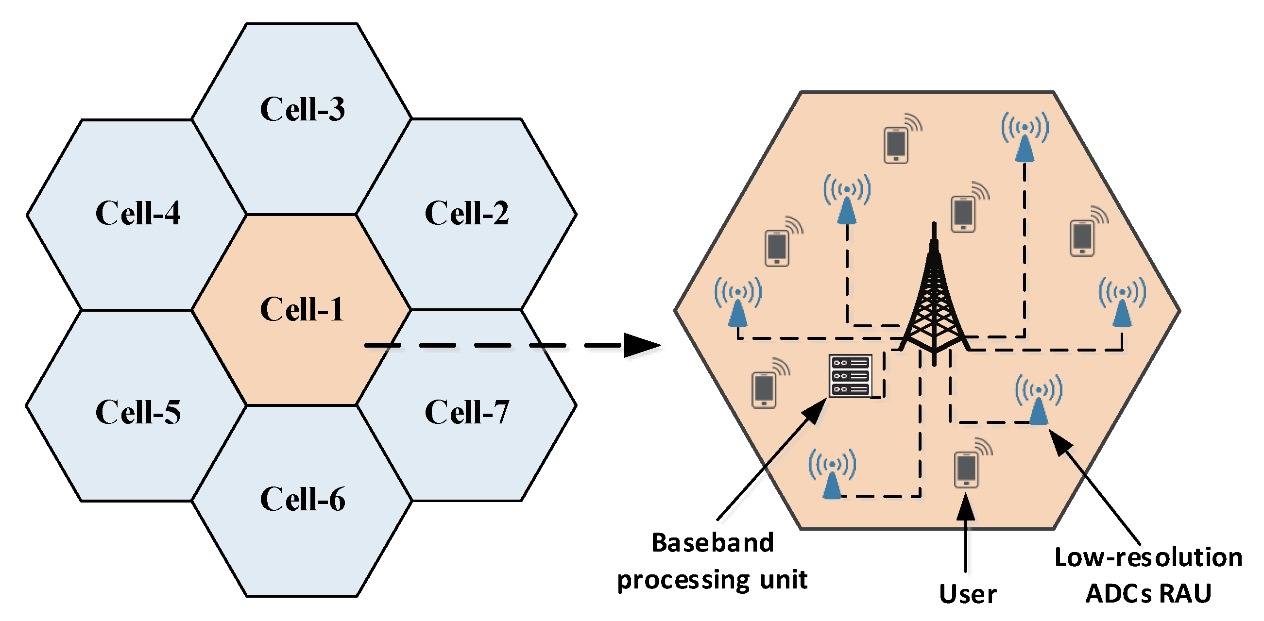
2. System Model

We consider a distributed massive MIMO system. There are L adjacent cells, and each cell consists of M remote antennas units (RAUs) and K single-antenna users. Each RAU is equipped with an array of N antennas. Each antenna is equipped with a low-resolution ADC, which means system performance will be degraded by quantization noise. RAUs in the same cell transmit or receive signals simultaneously while the beamforming design and signal processing are performed in a baseband processing unit. An example is given in Figure 1. There are L = 7 adjacent cells, and in cell-1, there are K = 6 users and M = 6 RAUs.

2.1. Quantization Noise Model

For uplink transmission, the signal vector received by all RAUs in cell l can be given by
y l = p u i = 1 L G l , i x i + n l ,
where x i is the K × 1 signal vector transmitted by the K users in cell i, p u is the uplink transmitted power, and n l CN ( 0 , I M N ) is the additive white Gaussian noise, G l , i = [ g l , i , 1 , . . . , g l , i , K ] is the M N × K channel matrix from M RAUs in cell l to K users in cell i, wherein
g l , i , k = λ l , 1 , i , k h l , 1 , i , k T , , λ l , M , i , k h l , M , i , k T T
where λ l , m , i , k is the path loss between the k-th user in the i-th cell and the m-th RAU in the l-th cell, which is dependent on the corresponding distance, and h l , m , i , k CN ( 0 , I N ) denotes the small scale fading.
This paper assumes that the CSI is unknown to the base station, and pilot training is performed. Motivated by [21], based on the minimum mean square error (MMSE) channel estimation, the equivalent estimated channel can be given by
g ^ i , l , k = β i , 1 , l , k h ^ i , k , 1 T , , β i , M , l , k h ^ i , k , M T T
where
β i , m , l , k = λ i , m , l , k 2 j = 1 L λ i , m , j , k + 1 / ( τ p u ) .
τ denotes the length of pilot sequences, β i , m , l , k denotes the equivalent path loss between the k-th user in the l-th cell and the m-th RAU in the i-th cell, and h ^ i , k = Δ [ h ^ i , k , 1 T , , h ^ i , k , M T ] T CN 0 , I M N represents the equivalent small scale fading part of the estimated channel. Because of the orthogonality principle of MMSE estimation theory, g i , l , k can be decomposed as
g i , l , k = g ^ i , l , k + g ˜ i , l , k
where g ˜ i , l , k CN 0 , diag η i , 1 , l , k , , η i , M , l , k I N is the uncorrelated and statistically independent of g ^ i , l , k estimation error, and η i , m , l , k = Δ λ i , m , l , k β i , m , l , k .
After the received analog signals pass through the low-resolution ADCs, the quantized digital signal vector can be obtained as
y l , q = Q ( y l ) = Q p u i = 1 L G l , i x i + n l
where Q ( . ) represents the quantization function. Assuming that the gain of automatic gain control is appropriately set, the additive quantization noise model (AQNM) can be employed to reformulate the quantized signal vector as
y l , q = α y l + n l , q = α p u i = 1 L G l , i x i + α n l + n l , q
where α = 1 ρ , ρ is the inverse of the signal-to-quantization-noise ratio, and n l , q denotes the additive uncorrelated quantization noise vector, which is Gaussian-distributed. The parameter ρ is a constant dependent on the number of quantization bits b. According to [16], the covariance matrix of quantization noise n l , q for a fixed channel realization can be denoted as
R n l , q = α ( 1 α ) diag p u i = 1 L G l , i G l , i H + I .

2.2. The Energy Efficiency Model

(1) Achievable uplink rates: In the uplink transmission phase, the quantized signal processed by the linear detector of user k in cell l is presented as
r l , k = a l , k H y l , q = α p u i = 1 L j = 1 K a l , k H g ^ l , i , j x i , j + α p u i = 1 L j = 1 K a l , k H g ˜ l , i , j x i , j + α a l , k H n l + α a l , k H n l , q
where a l , k is the linear receiver vector in cell l for user k, and x i , j CN ( 0 , 1 ) is the j-th column of x i . In this paper, we focus on two linear receivers, namely MRC and ZF. Mathematically, a l , k can be given by
a l , k = g ^ l , l , k , for MRC f l , l , k , for ZF
where f l , l , k is the k-th column of G ^ l , l G ^ l , l H G ^ l , l 1 , and G ^ l , l = g ^ l , l , 1 , , g ^ l , l , K .
Motivated by [22,23], treating the interference as worst-case unrelated additive noise, the lower bound of the achievable uplink rate of the k-th user in the l-th cell can be given by
R l , k ( p ) = E log 2 1 + p u α 2 | a l , k H g ^ l , l , k | 2 E a l , k H p u α 2 ( i , j ) ( l , k ) g ^ l , i , j g ^ l , i , j H + p u α 2 ( i , j ) g ˜ l , i , j g ˜ l , i , j H + α 2 + R n l , q a l , k | G ^ l , l
= ( a ) E log 2 1 + p u α 2 | a l , k H g ^ l , l , k | 2 E I l , k + p u α 2 i l | a l , k H g ^ l , i , k | 2 + α 2 a l , k H 2
where p is the transmitted power vector of K users. Since the denominator of Equation (11) is a conditional expectation operator and the estimated error vector and estimated channel vector are independent, I l , k is given as
I l , k = p u α 2 i = 1 L j k a l , k H E g ^ l , i , j g ^ l , i , j H a l , k + p u α 2 ( i , j ) a l , k H E g ˜ l , i , j g ˜ l , i , j H a l , k + a l , k H E R n l , q a l , k
wherein
E g ^ l , i , j g ^ l , i , j H = diag β l , 1 , i , j I N , , β l , M , i , j I N E g ˜ l , i , j g ˜ l , i , j H = diag η l , 1 , i , j I N , , η l , M , i , j I N E R n l , q = diag p u G ^ l , l G ^ l , l H + D R D R = diag p u j = 1 K η l , 1 , l , j + p u i l j = 1 K λ l , 1 , i , j + 1 I N , , p u j = 1 K η l , M , l , j + p u i l j = 1 K λ l , M , i , j + 1 I N . η l , m , i , j = η l , m , i , j β l . m , i , j .
(2) Power consumption model: According to [24,25,26], for cell l, the total power consumption model can be given by
P l = P TC + P LP + P T + P BH .
The first term P TC is the power consumption of transceiver chains, which can be given by
P TC = M ( N P BS + ρ P SYN ) + ( 1 ρ ) P SYN + K P UE + M P ADC
where P BS and P UE are the power consumption of running the circuit components employed at the base station and users, P SYN are the power consumed by the local oscillator, and P ADC = a 0 N 2 b + a 1 are the power consumed by ADC, wherein a 0 and a 1 are constant parameters, ρ = 1 for the distributed antenna system (DAS), and ρ = 0 for the co-located antenna system (CAS). This results from the assumption that antennas at the same RAU are connected to a common oscillator, while oscillators at different RAUs are different in the DAS, and all antennas are connected to a single oscillator in the CAS.
The second term P LP is the power consumption of the MRC/ZF receiver at the base station, which can be given by
P LP = B T τ T 2 M N K L BS + B T 3 M N K L BS ( 1 d ) + d K 3 3 L BS + M N K ( 3 K + 1 ) L BS
where d = 0 for MRC while d = 1 for ZF, B is the bandwidth, T denotes the symbols for uplink transmission, and L BS is the computational efficiency of arithmetic complex-valued operations for a Joule.
The third term P T is transmit power, which can be represented as
P T = T τ T K ξ p u
where ξ is the amplified efficiency.
For the last term, P BH is the power consumed of backhaul in the DAS, while it can be neglected in the CAS. Specifically, P BH in the DAS can be given by
P BH = M P 0 + B P BT k = 1 K R l , k ( p )
where P 0 and P BT are the fixed and traffic-dependent power consumption at each backhaul, respectively.
(3) Global energy efficiency model: Based on the above analysis, the total power consumption for all cells can be given by
P Total ( p ) = L P IND + T τ ξ T L K p u + P BT M B l = 1 L k = 1 K R l , k ( p )
where P IND is the power consumption independent of p and can be given by
P IND = P TC + P LP + M P 0 .
According to [24], the global energy efficiency is defined as the ratio of the achievable sum rate to the total power consumption in Watts. Mathematically, it can be defined as
φ ( p ) = B l = 1 L k = 1 K R l , k ( p ) P Total .

3. Energy Efficiency Analysis

From Equations (22) and (A4), we can see that it is difficult to directly calculate Equation (A4) to analyze the energy efficiency. Therefore, we first derive the closed-form expressions of uplink achievable rates. The results are shown in the following theorems.
Theorem 1.
Using MRC receiver with low-resolution ADCs and pilot contamination, the closed-form expression for the uplink achievable rate of the k-th user in the l-th cell is given by
R l , k mrc = log 2 1 + p u α N m = 1 M β l , m , l , k 2 + N m = 1 M β l , m , l , k 2 p u α Ω l , k + p u α Ξ l , k + ( 1 α ) Φ l , k + α m = 1 M β l , m , l , k 2
where
Ω l , k = N m = 1 M i = 1 L j = 1 K β l , m , l , k η l , m , i , j Ξ l , k = N m = 1 M β l , m , l , k i = 1 L j k β l , m , i , j + i l β l , m , i , k + i l N m = 1 M β l , m , l , k 1 / 2 β l , m , i , k 1 / 2 2 Φ l , k = p u N m = 1 M β l , m , l , k 2 + N m = 1 M β l , m , l , k 2 + N j k m = 1 M β l , m , l , k β l , m , l , j + Υ l , k Υ l , k = N m = 1 M β l , m , l , k 1 + p u j = 1 K η l , m , l , j + p u i l j = 1 K λ l , m , i , j .
Proof. 
The proof is given in Appendix B. □
Theorem 2.
Using ZF receiver with low-resolution ADCs and pilot contamination, the closed-form expression for the uplink achievable rate of user k in the l-th cell is given by
R l , k zf = log 2 1 + p u α ζ m = 1 M β l , m , l , k α p u m = 1 M i l j k β l , m , i , j + i = 1 L j = 1 K η l , m , i , j + ζ i l β l , m , i , k + ( 1 α ) ζ p u m = 1 M β l , m , l , k + Δ l , k + α M
where ζ = M N K + 1 , and
Δ l , k = m = 1 M 1 + p u j = 1 K η l , m , l , j + p u i l j = 1 K λ l , m , i , j .
Proof. 
The proof is given in Appendix C. □
From Equations (23) and (25), it can be concluded that the quantization noise influences both the numerator and the denominator of Equation (A4). This means that the quantization noise is unlike the additive noise, which only affects the denominator.
Based on the theorems above, we analyze the asymptotic performance with quantization bits, per user transmit power, and the number of antennas per RAU, respectively. The results are given below.
Case 1: With a fixed transmitted power per user p u and a total number of antennas per cell M N , when the number of quantization bits b , the inverse of the signal-to-quantization-noise ratio ρ tends toward zero, which means that α in Equations (23) and (25) tends toward 1. The following results can then be obtained in this case by replacing the α in Equations (23) and (25) with 1
R ˜ l , k mrc = log 2 1 + p u N m = 1 M β l , m , l , k 2 + N m = 1 M β l , m , l , k 2 p u Ω l , k + p u Ξ l , k + m = 1 M β l , m , l , k 2
R ˜ l , k zf = log 2 1 + p u ζ m = 1 M β l , m , l , k p u m = 1 M i l j k β l , m , i , j + i = 1 L j = 1 K η l , m , i , j + ζ i l β l , m , i , k + M .
Case 1 shows the achievable uplink rates without considering the quantization noise caused by ADC. It can be seen that the spectral efficiency is only limited by pilot contamination and channel estimation error. Moreover, since the power consumption of an ADC P ADC = a 0 N 2 b + a 1 is an exponential function of b, P ADC tends toward infinity when b . As shown in Equation (20), the total power consumption also goes to infinity. Hence, the limited achievable rates and unlimited power consumption lead to the fact that the global energy efficiency tends toward zero, that is ϕ ( p ) 0 when b , while p u and M N are fixed.
Case 2: With a fixed number of quantization bits b and antennas per cell M N , when p u , the ultimate rates of user k in cell l with both receivers can be directly obtained by dividing the dominators and numerators of Equations (23) and (25) by p u , which are given by
R ˜ l , k mrc = log 2 1 + α N m = 1 M β l , m , l , k 2 + N m = 1 M β l , m , l , k 2 α Ω l , k + α Ξ l , k + ( 1 α ) Φ l , k
R ˜ l , k zf = log 2 1 + α ζ m = 1 M β l , m , l , k α m = 1 M i l j k β l , m , i , j + i = 1 L j = 1 K η l , m , i , j + ζ i l β l , m , i , k + ( 1 α ) ζ m = 1 M β l , m , l , k + Δ l , k
where
Φ l , k = N m = 1 M β l , m , l , k 2 + N m = 1 M β l , m , l , k 2 + N j k m = 1 M β l , m , l , k β l , m , l , j + Υ l , k Υ l , k = N m = 1 M β l , m , l , k j = 1 K η l , m , l , j + i l j = 1 K λ l , m , i , j Δ l , k = m = 1 M j = 1 K η l , m , l , j + i l j = 1 K λ l , m , i , j .
Case 2 indicates that, as p u grows indefinitely, the achievable uplink rates approach certain values dependent on the resolution of ADC. This observation shows that the performance degradation due to low-resolution ADCs cannot be compensated by increasing the transmit power. Furthermore, it can be seen that, as the transmit power increases, the system energy efficiency tends toward zero. This is because the total power consumption presented in Equation (20) tends toward infinity as p u increases indefinitely, but the unlimited growth in the transmit power cannot improve the achievable uplink rates indefinitely.
Case 3: With a fixed number of quantization bits b, the number of RAUs per cell M and the transmitted power per user p u , when N , the limiting rates of user k in cell l with both receivers can be directly obtained by dividing the dominators and numerators of Equations (23) and (25) by N 2 , which are given by
R l , k mrc = log 2 1 + α m = 1 M β l , m , l , k 2 α i l m = 1 M β l , m , l , k 1 / 2 β l , m , i , k 1 / 2 2 + ( 1 α ) m = 1 M β l , m , l , k 2
R l , k zf = log 2 1 + α m = 1 M β l , m , l , k α i l m = 1 M β l , m , i , k + ( 1 α ) m = 1 M β l , m , l , k .
Case 3 shows that, when the number of antennas per RAU grows without bound, the impacts of quantization noise vanish. However, the achievable rates with both receivers tend toward certain and limited values as N goes infinity. This results from the presence of pilot contamination. Furthermore, since the power consumption of transceiver chains and linear processing at the base station are proportional to N, they tend toward infinity when N . As shown in Equation (20), the total power consumption also goes to infinity. Hence, the limited achievable rates and unlimited power consumption lead to the fact that the global energy efficiency tends toward zero, that is ϕ ( p ) 0 when N while b, M, and p u are fixed.

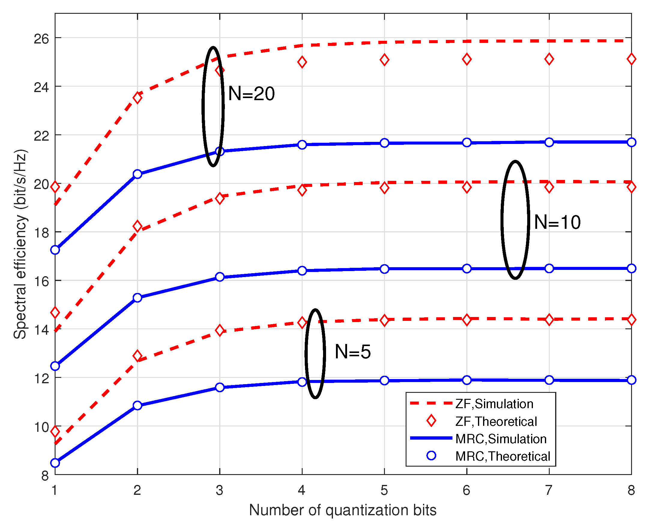
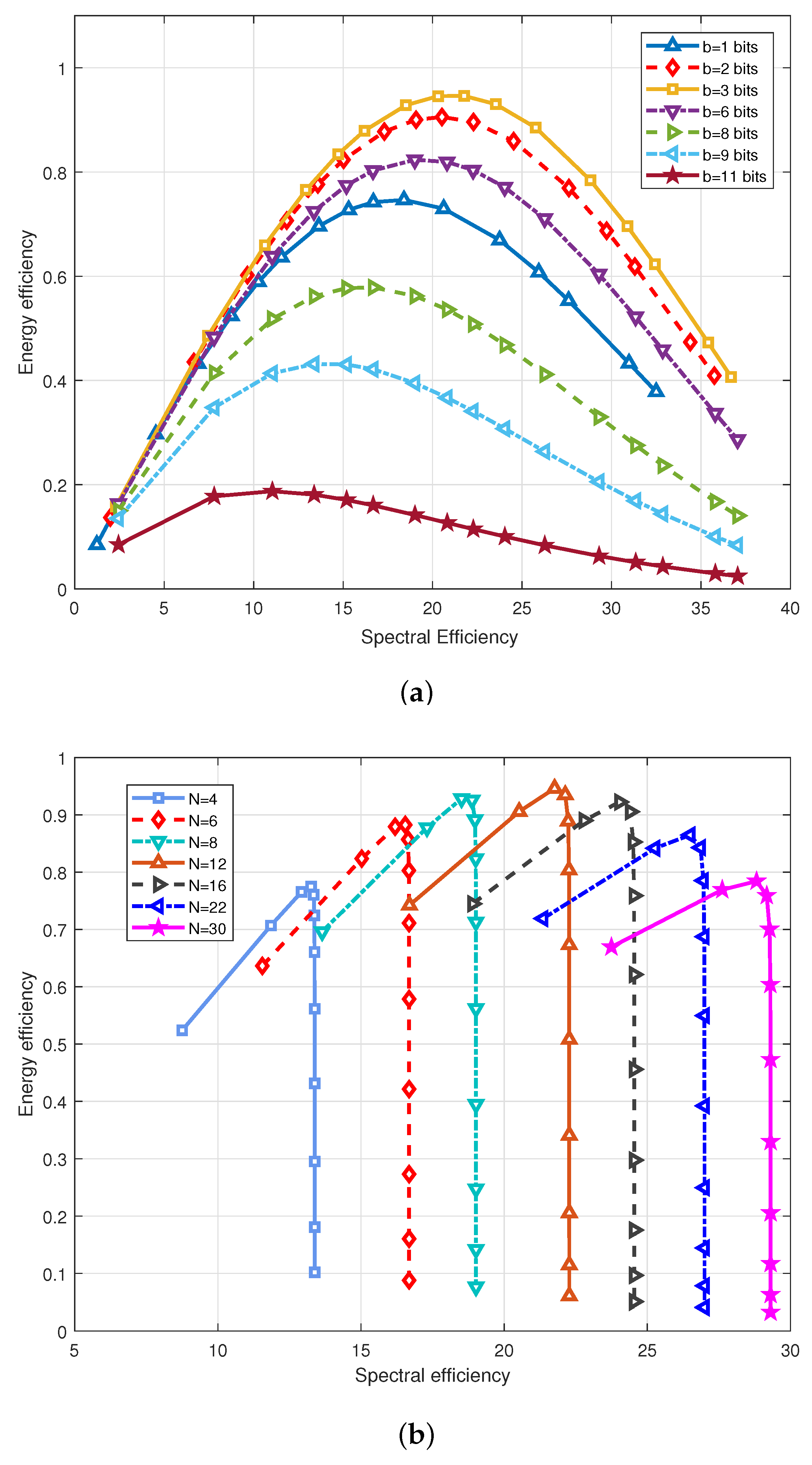
4. Numerical Results

In this section, we verify the accuracy of the theoretical results in Section 3 by a series of Monte Carlo simulations. A multi-cell distributed massive MIMO system is considered, which consists of L = 7 cells, M = 7 RAUs per cell, K = 6 users per cell, and the cell radius D is normalized to 1. In each cell, all users are uniformly distributed, while RAUs have fixed locations with radiuses r 1 = 0 , r 2 = = r 7 = ( 3 3 ) / 2 and angles θ 1 = 0 , θ 2 = π / 6 , θ 3 = π / 2 , θ 4 = 5 π / 6 , θ 5 = 7 π / 6 , θ 6 = 3 π / 2 , a n d   θ 7 = 11 π / 6 . The path loss between the k-th user in the i-th cell and the m-th RAU in the l-th cell λ l , m , i , k is modeled as λ l , m , i , k = d l , m , i , k ι , where d l , m , i , k is the corresponding distance, and ι assumed as ι = 3 . 7 is the path loss exponent. Moreover, the length of pilot sequences is τ = K . The coherence time of the channel is assumed as T = 196 symbols, and the power consumption parameters are given in Table 1.
We first prove the accuracy of the theoretical results given in Theorems 1 and 2. Figure 2 illustrates the uplink spectral efficiency per cell versus the number of quantization bits with different numbers of antennas per RAU. It can be seen that the closed-form expressions and simulation results match well with each other using both MRC and ZF receivers. As the number of antennas per RAU increases, the uplink spectral efficiency grows obviously for both receivers. Furthermore, for both receivers, the uplink spectral efficiency increases rapidly with the increase in quantization bits b when b is small, while the growth of b cannot improve the spectral efficiency further when b is large. It can be concluded that low-resolution ADCs are acceptable in massive MIMO systems, and employing a large number of antennas at each RAU can compensate for the performance degradation. In the following, the closed-form expressions will be used for numerical work.
Next, Figure 3 illustrates the energy efficiency versus spectral efficiency with different numbers of quantization bits and of antennas per RAU. It can be seen that, as the number of antennas and the number of quantization bits increase, energy efficiency increases first and then decreases. This is because the power consumption and spectral efficiency both increase with the increase in antennas and quantization bits, but the improvement of spectral efficiency dominates first, and the power consumption then dominates. The results illustrate that we cannot improve the spectral efficiency and energy efficiency simultaneously without bound, and there needs to be a tradeoff between them, which was investigated in [27,28,29]. Moreover, it can be seen in Figure 3b that b = 3 or b = 4 are preferable under the system configuration mentioned above. If b increases further, the spectral efficiency can be slightly improved while the energy efficiency decreases rapidly. It should be noted that the optimal number of bits is dependent on system configuration and system parameters. Figure 3 also indicates that low-resolution ADCs (b = 3 or 4 bits in our simulation results) are preferable in distributed massive MIMO systems.
Finally, the energy efficiency against spectral efficiency with different numbers of quantization bits and transmitted power per user is presented in Figure 4. The same conclusion about the relationship between energy efficiency and spectral efficiency with different b can be obtained from Figure 4. As for the transmitted power per user, it can be seen that, with its increase, the energy efficiency increases first and then decreases. This results from the fact that the power consumption linearly increases with the growth of transmitted power, but the spectral efficiency increases first and then tends toward a certain value.

5. Conclusions

In this paper, we analyzed the uplink spectral and energy efficiency simultaneously in distributed massive MIMO systems with low-resolution ADCs. Furthermore, this paper considered a more realistic scenario where the base station did not have CSI and it obtained the estimated CSI during the pilot phase. In this case, the pilot contamination presents and degrades the system performance. We first gave an additive quantization noise model and got the estimated CSI with pilot contamination. Under the imperfect CSI, we derived the closed-form expressions for achievable uplink rates using MRC and ZF receivers. Furthermore, we obtained the asymptotic performance with the number of quantization bits, the per user transmit power, and the per RAU antenna number, respectively. The theorems are verified by simulation. It can be noted that the increase in antennas can compensate for the spectral efficiency degradation caused by quantization noise. Furthermore, the energy efficiency with low-resolution ADCs are better than that with perfect ADCs. Numerical results imply that it is preferable to use low-resolution ADCs in distributed massive MIMO systems.
We intend to extend our research considering the tradeoff between spectral efficiency and energy efficiency, which involves multi-objective optimization. Furthermore, in order to make the system more energy-efficient, we plan to extend our research considering RAU selection.

Author Contributions

Formal analysis, J.L.; Methodology, J.L.; Supervision, P.Z. and X.Y.; Validation, J.L. and J.Y.; Writing original draft, J.L. and Q.L.; Writing review & editing, J.L. and Q.L.

Funding

This work was supported in part by National Natural Science Foundation of China (NSFC) (Grant No. 61501113, 61571120) and the Jiangsu Provincial Natural Science Foundation (Grant No. BK20150630, BK20180011).

Conflicts of Interest

The authors declare no conflict of interest.

Appendix A. Lemmas for Proof

In order to derive the closed-form expressions with both receivers, we provide the following preliminary lemmas first.
Lemma A1 
([22]) Suppose { X i } are independent Gamma distributed random variables, i.e., { X i } Γ ( k i , θ i ) . Then the first two moments of the sum i X i can be given by
E i X i = i k i θ i ,
E i X i 2 = i k i θ i 2 + i k i θ i 2 .
Lemma A2 
([21]) For the p-dimensional non-isotropic channel vector x whose strength is distributed as x H x Γ ( k , θ ) , when projected onto a s-dimensional subspace, the distribution of the projection power can be approximated as Γ ( s k / p , θ ) .
Lemma A3 
([30]) If x is an N × 1 isotropic random vector and A is a constant matrix. Then we can have
E x x H A x = tr ( A ) N .

Appendix B. Proof of Theorem 1

From Lemma 4 of [31], we can obtain the approximation of Equation (11) as follows:
R l , k ( p ) log 2 1 + p u α 2 E | a l , k H g ^ l , l , k | 2 E I l , k + p u α 2 i l | a l , k H g ^ l , i , k | 2 + α 2 a l , k H 2 .
Consider the MRC receiver, it can be seen from Equation (A4) that the following terms need to be simplified:
E g ^ l , l , k 4 = k ^ l , l , k θ ^ l , l , k 2 + ( k ^ l , l , k θ ^ l , l , k ) 2
where
k ^ l , l , k = N ( m = 1 M β l , m , l , k ) 2 m = 1 M β l , m , l , k 2 θ ^ l , l , k = m = 1 M β l , m , l , k 2 m = 1 M β l , m , l , k .
This can be obtained by exploiting the fact that g ^ l , l , k H g ^ l , l , k Γ ( k ^ l , l , k , θ ^ l , l , k ) and Lemma A1.
Due to the independence between g ^ l , l , k and g ^ l , i , j when j k , we have
E g ^ l , l , k H E g ^ l , i , j g ^ l , i , j H g ^ l , l , k = ( a ) N m = 1 M β l , m , l , k β l , m , i , j
where ( a ) results from the fact that the channel strength is Gamma-distributed.
Because of the pilot contamination, g ^ l , l , k and g ^ l , i , k are dependent, we have
E | g ^ l , l , k H g ^ l , i , k | 2 = ( a ) N m = 1 M β l , m , l , k 1 / 2 β l , m , i , k 1 / 2 2 + N m = 1 M β l , m , l , k β l , m , i , k
where (a) is obtained due to the fact that the channel strength is Gamma-distributed and due to Lemma A1.
Using the fact that g ^ l , l , k and g ˜ l , i , j are independent, we have
( i , j ) E g ^ l , l , k H E g ˜ l , i , j g ˜ l , i , j H g ^ l , l , k = N m = 1 M i = 1 L j = 1 K β l , m , l , k η l , m , i , j .
For the last term, we first calculate
E g ^ l , l , k H diag p u G ^ l , l G ^ l , l H g ^ l , l , k = p u E g ^ l , l , k H g ^ l , l , k g ^ l , l , k H g ^ l , l , k + p u j k E g ^ l , l , k H g ^ l , l , j g ^ l , l , j H g ^ l , l , k = p u k ^ l , l , k θ ^ l , l , k 2 + ( k ^ l , l , k θ ^ l , l , k ) 2 + N j k m = 1 M β l , m , l , k β l , m , l , j .
Then we can obtain
E g ^ l , l , k H E diag p u i = 1 L G l , i G l , i H + I g ^ l , l , k = E g ^ l , l , k H diag p u G ^ l , l G ^ l , l H g ^ l , l , k + E n = 1 M N g ^ l , n , l , k 2 D R = p u k ^ l , l , k θ ^ l , l , k 2 + ( k ^ l , l , k θ ^ l , l , k ) 2 + N j k m = 1 M β l , m , l , k β l , m , l , j + Υ l , k .
Substituting Equations (A5), (A7)–(A9), and (A11) into Equation (A4) yields the closed-form expression expressed by Equation (23). This completes the proof.

Appendix C. Proof of the Theorem 2

Consider a ZF receiver, similar to the proof of Theorem 1. The following terms need to be calculated.
For the term E 1 a l , k H 2 , we have
1 a l , k H 2 = a l , k H a l , k H 2 g ^ l , l , k Γ M N K + 1 M N k ^ l , l , k , θ ^ l , l , k ,
which results form Lemma A2 and from the fact that, from the perspective of each user, an intended beam lies in a subspace of dimension s = M N K + 1 with ZF receivers. Thus,
E 1 a l , k H 2 = M N K + 1 M N k ^ l , l , k θ ^ l , l , k .
Next, due to the independence between a l , k and g ^ l , i , j , we have
i l j k E a l , k H E g ^ l , i , j g ^ l , i , j H a l , k = ( a ) i l j k E E a l , k H g ^ l , i , j g ^ l , i , j H a l , k = ( b ) 1 M N E g ^ l , i , j H g ^ l , i , j = ( c ) 1 M i l j k m = 1 M β l , m , i , j .
where (a) results from the fact that a l , k and g ^ l , i , j are independent, (b) results from Lemma A3, and (c) results from the fact that g ^ l , i , j H g ^ l , i , j Γ ( k ^ l , i , j , θ ^ l , i , j ) .
Similarly, we have
( i , j ) E a l , k H a l , k H 2 E g ˜ l , i , j g ˜ l , i , j H a l , k a l , k H 2 = 1 M i = 1 L j = 1 K m = 1 M η l , m , i , j .
Due to the pilot contamination, a l , k and g ^ l , i , k are dependent, we have
i l E a l , k H a l , k H g ^ l , i , k 2 = M N K + 1 M i l m = 1 M β l , m , i , k .
For the last term, we first calculate
E a l , k H a l , k H diag p u G ^ l , l G ^ l , l H a l , k a l , k H = p u E a l , k H a l , k H g ^ l , l , k g ^ l , l , k H a l , k a l , k H = M N K + 1 M N p u k ^ l , l , k θ ^ l , l , k .
Then we can obtain
E a l , k H a l , k H E diag p u i = 1 L G l , i G l , i H + I a l , k a l , k H = E a l , k H a l , k H diag p u G ^ l , l G ^ l , l H a l , k a l , k H + E a l , k H a l , k H D R a l , k a l , k H = ( a ) M N K + 1 M N p u k ^ l , l , k θ ^ l , l , k + 1 M Δ l , k
where ( a ) results form Lemma A3.
Substituting Equations (A13)–(A16), and (A18) into Equation (A4) yields the closed-form expression expressed by Equation (25). This completes the proof.

References

  1. Wang, J.; Zhu, H.; Gomes, N.J.; Wang, J. Frequency Reuse of Beam Allocation for Multiuser Massive MIMO Systems. IEEE Trans. Wirel. Commun. 2018, 17, 2346–2359. [Google Scholar] [CrossRef]
  2. Marzetta, T.L. Noncooperative Cellular Wireless with Unlimited Numbers of Base Station Antennas. IEEE Trans. Wirel. Commun. 2010, 9, 3590–3600. [Google Scholar] [CrossRef]
  3. Larsson, E.G.; Edfors, O.; Tufvesson, F.; Marzetta, T.L. Massive MIMO for next generation wireless systems. IEEE Commun. Mag. 2014, 52, 186–195. [Google Scholar] [CrossRef] [Green Version]
  4. Lu, L.; Li, G.Y.; Swindlehurst, A.L.; Ashikhmin, A.; Zhang, R. An Overview of Massive MIMO: Benefits and Challenges. IEEE J. Sel. Top. Signal Process. 2014, 8, 742–758. [Google Scholar] [CrossRef]
  5. Wang, D.; Zhang, Y.; Wei, H.; You, X.; Gao, X.; Wang, J. An overview of transmission theory and techniques of large-scale antenna systems for 5G wireless communications. Sci. China Inf. Sci. 2016, 59, 081301. [Google Scholar] [CrossRef]
  6. Zhang, J.; Wen, C.; Jin, S.; Gao, X.; Wong, K. On Capacity of Large-Scale MIMO Multiple Access Channels with Distributed Sets of Correlated Antennas. IEEE J. Sel. Areas Commun. 2013, 31, 133–148. [Google Scholar] [CrossRef] [Green Version]
  7. Rusek, F.; Persson, D.; Lau, B.K.; Larsson, E.G.; Marzetta, T.L.; Edfors, O.; Tufvesson, F. Scaling Up MIMO: Opportunities and Challenges with Very Large Arrays. IEEE Signal Process. Mag. 2013, 30, 40–60. [Google Scholar] [CrossRef] [Green Version]
  8. Li, J.; Wang, D.; Zhu, P.; Wang, J.; You, X. Downlink Spectral Efficiency of Distributed Massive MIMO Systems With Linear Beamforming Under Pilot Contamination. IEEE Trans. Veh. Technol. 2018, 67, 1130–1145. [Google Scholar] [CrossRef] [Green Version]
  9. Björnson, E.; Matthaiou, M.; Debbah, M. Massive MIMO with non-ideal arbitrary arrays: Hardware scaling laws and circuit-aware design. IEEE Trans. Wirel. Commun. 2015, 14, 4353–4368. [Google Scholar] [CrossRef]
  10. Zhu, H. Performance Comparison Between Distributed Antenna and Microcellular Systems. IEEE J. Sel. Areas Commun. 2011, 29, 1151–1163. [Google Scholar] [CrossRef]
  11. You, X.H.; Wang, D.M.; Sheng, B.; Gao, X.Q.; Zhao, X.S.; Chen, M. Cooperative distributed antenna systems for mobile communications. IEEE Wirel. Commun. 2010, 17, 35. [Google Scholar] [CrossRef]
  12. Dai, L. A Comparative Study on Uplink Sum Capacity with Co-Located and Distributed Antennas. IEEE J. Sel. Areas Commun. 2011, 29, 1200–1213. [Google Scholar] [CrossRef]
  13. Bai, Q.; Nossek, J.A. Energy efficiency maximization for 5G multi-antenna receivers. Trans. Emerg. Telecommun. Technol. 2015, 26, 3–14. [Google Scholar] [CrossRef]
  14. Walden, R.H. Analog-to-digital converter survey and analysis. IEEE J. Sel. Areas Commun. 1999, 17, 539–550. [Google Scholar] [CrossRef] [Green Version]
  15. Singh, J.; Dabeer, O.; Madhow, U. On the limits of communication with low-precision analog-to-digital conversion at the receiver. IEEE Trans. Commun. 2009, 57, 3629–3639. [Google Scholar] [CrossRef] [Green Version]
  16. Fan, L.; Jin, S.; Wen, C.; Zhang, H. Uplink Achievable Rate for Massive MIMO Systems With Low-Resolution ADC. IEEE Commun. Lett. 2015, 19, 2186–2189. [Google Scholar] [CrossRef]
  17. Qiao, D.; Tan, W.; Zhao, Y.; Wen, C.; Jin, S. Spectral efficiency for massive MIMO zero-forcing receiver with low-resolution ADC. In Proceedings of the 2016 8th International Conference on Wireless Communications Signal Processing (WCSP), Yangzhou, China, 13–15 October 2016; pp. 1–6. [Google Scholar] [CrossRef]
  18. Verenzuela, D.; Bjrnson, E.; Matthaiou, M. Hardware design and optimal ADC resolution for uplink massive MIMO systems. In Proceedings of the 2016 IEEE Sensor Array and Multichannel Signal Processing Workshop (SAM), Rio de Janerio, Brazil, 10–13 July 2016; pp. 1–5. [Google Scholar] [CrossRef]
  19. Sarajlić, M.; Liu, L.; Edfors, O. When Are Low Resolution ADCs Energy Efficient in Massive MIMO? IEEE Access 2017, 5, 14837–14853. [Google Scholar] [CrossRef]
  20. Roth, K.; Nossek, J.A. Achievable Rate and Energy Efficiency of Hybrid and Digital Beamforming Receivers With Low Resolution ADC. IEEE J. Sel. Areas Commun. 2017, 35, 2056–2068. [Google Scholar] [CrossRef] [Green Version]
  21. Li, J.; Wang, D.; Zhu, P.; You, X. Uplink Spectral Efficiency Analysis of Distributed Massive MIMO With Channel Impairments. IEEE Access 2017, 5, 5020–5030. [Google Scholar] [CrossRef]
  22. Li, J.; Wang, D.; Zhu, P.; You, X. Spectral efficiency analysis of single-cell multi-user large-scale distributed antenna system. IET Commun. 2014, 8, 2213–2221. [Google Scholar] [CrossRef]
  23. Ngo, H.Q.; Larsson, E.G.; Marzetta, T.L. Energy and Spectral Efficiency of Very Large Multiuser MIMO Systems. IEEE Trans. Commun. 2013, 61, 1436–1449. [Google Scholar] [CrossRef] [Green Version]
  24. Zuo, J.; Zhang, J.; Yuen, C.; Jiang, W.; Luo, W. Energy-Efficient Downlink Transmission for Multicell Massive DAS With Pilot Contamination. IEEE Trans. Veh. Technol. 2017, 66, 1209–1221. [Google Scholar] [CrossRef] [Green Version]
  25. Ngo, H.Q.; Tran, L.; Duong, T.Q.; Matthaiou, M.; Larsson, E.G. On the Total Energy Efficiency of Cell-Free Massive MIMO. IEEE Trans. Green Commun. Netw. 2018, 2, 25–39. [Google Scholar] [CrossRef] [Green Version]
  26. Björnson, E.; Sanguinetti, L.; Hoydis, J.; Debbah, M. Optimal Design of Energy-Efficient Multi-User MIMO Systems: Is Massive MIMO the Answer? IEEE Trans. Wirel. Commun. 2015, 14, 3059–3075. [Google Scholar] [CrossRef] [Green Version]
  27. Pham, Q.; Hwang, W. Fairness-Aware Spectral and Energy Efficiency in Spectrum-Sharing Wireless Networks. IEEE Trans. Veh. Technol. 2017, 66, 10207–10219. [Google Scholar] [CrossRef]
  28. Deng, L.; Rui, Y.; Cheng, P.; Zhang, J.; Zhang, Q.T.; Li, M. A Unified Energy Efficiency and Spectral Efficiency Tradeoff Metric in Wireless Networks. IEEE Commun. Lett. 2013, 17, 55–58. [Google Scholar] [CrossRef]
  29. Xu, L.; Yu, G.; Jiang, Y. Energy-Efficient Resource Allocation in Single-Cell OFDMA Systems: Multi-Objective Approach. IEEE Trans. Wirel. Commun. 2015, 14, 5848–5858. [Google Scholar] [CrossRef]
  30. Heath, W.H., Jr.; Wu, T.; Kwon, Y.H.; Soong, A.C.K. Multiuser MIMO in Distributed Antenna Systems With Out-of-Cell Interference. IEEE Trans. Signal Process. 2011, 59, 4885–4899. [Google Scholar] [CrossRef]
  31. Lim, Y.; Chae, C.; Caire, G. Performance Analysis of Massive MIMO for Cell-Boundary Users. IEEE Trans. Wirel. Commun. 2015, 14, 6827–6842. [Google Scholar] [CrossRef]
Figure 1. System configuration.
Electronics 07 00391 g001
Figure 2. Spectral efficiency versus the number of quantization bits with different numbers of antennas per RAU.
Electronics 07 00391 g002
Figure 3. Energy efficiency versus spectral efficiency with different numbers of quantization bits b and different numbers of antennas N per RAU. (a) Each line corresponds to different numbers of quantization bits with b = [1, 2, 3, 6, 8, 9, 11] and the points on each line correspond to different numbers of antennas per RAU with N= [1:1:6, 8, 10, 12, 15, 20, 30, 40, 50, 80, 100]. (b) Each line corresponds to different numbers of antennas per RAU with N= [4, 6, 8, 12, 16, 22, 30] and the points on each line correspond to different numbers of quantization bits with b = [1:1:12].
Electronics 07 00391 g003
Figure 4. Energy efficiency versus spectral efficiency with the number of quantization bits b = [1:1:6] bits and transmitted power per user p u = [ 0.01 , 0.02 , 0.05 , 0.08 , 0.1 , 0.15 , 0.2 , 0.3 , 0.4 , 0.6 , 0.8 , 1 ] W, where each line corresponds to different b and the points on each line correspond to different p u .
Electronics 07 00391 g004
Table 1. Power consumption parameters.
ParametersValues
Transmitted power per user p u 0.02 Watts
Power consumption per antenna at base station P BS 0.1 Watts
Power consumption per antenna at users P UE 0.1 Watts
Power consumption per local oscillator P SYN 1 Watts
Computational efficiency at base stations L BS 12.8 Gflops/Watt
Power amplified efficiency ξ 0.4
Fixed power consumption per backhaul P 0 0.825 Watts
Traffic-dependent backhaul power P BT 0.25 Watts/(Gbit/s)
Parameters of ADC a 0 & a 1 10 3 & 0.02

