Research on Air Confrontation Maneuver Decision-Making Method Based on Reinforcement Learning

Abstract

With the development of information technology, the degree of intelligence in air confrontation is increasing, and the demand for automated intelligent decision-making systems is becoming more intense. Based on the characteristics of over-the-horizon air confrontation, this paper constructs a super-horizon air confrontation training environment, which includes aircraft model modeling, air confrontation scene design, enemy aircraft strategy design, and reward and punishment signal design. In order to improve the efficiency of the reinforcement learning algorithm for the exploration of strategy space, this paper proposes a heuristic Q-Network method that integrates expert experience, and uses expert experience as a heuristic signal to guide the search process. At the same time, heuristic exploration and random exploration are combined. Aiming at the over-the-horizon air confrontation maneuver decision problem, the heuristic Q-Network method is adopted to train the neural network model in the over-the-horizon air confrontation training environment. Through continuous interaction with the environment, self-learning of the air confrontation maneuver strategy is realized. The efficiency of the heuristic Q-Network method and effectiveness of the air confrontation maneuver strategy are verified by simulation experiments.

1. Introduction

The intelligent air confrontation decision-making system can be effectively applied to automatic/autonomous simulated air confrontation, maneuver confrontation, anti-interception and various auxiliary decision-making systems of manned/unmanned aerial vehicles. The world’s major military powers are conducting in-depth research in this field. The intelligent decision-making system will, thus, become an important part of future decision on air confrontation.

In the process of over-the-horizon air confrontation, reasonable maneuver decision-making is the premise of making weapons attack, sensor use, electronic countermeasures, and other decisions. It is accompanied by the entire air confrontation process and is an extremely important part. This paper mainly studies the intelligent maneuver decision-making method in this environment, based on the single-to-single air confrontation confrontation in super-horizon air confrontation.

The current air confrontation decision-making methods can be divided into two main categories: non-learning strategies and self-learning strategies. Among them, the non-learning strategy mainly adopts the optimization theory or the game method. There is no data-based training process in the strategy solving process, and there is no process of updating and optimizing the strategy by interacting with the environment. The methods adopted by non-learning strategies mainly include: differential countermeasure [1,2], matrix game [3], expert system [4], and impact map [5] among others. The self-learning strategy refers to the information generated by the interaction between the historical data and the environment; and strategy learning is carried out, and finally a better strategy is solved. The self-learning strategy has characteristics of offline and online learning training, and has strong adaptability and can cope with complex and changeable environments. The main methods used in self-learning strategies include: genetic algorithm [6,7], artificial immune system [8,9], supervised learning [10], reinforcement learning [11], etc.

Reinforcement learning is a self-learning method which, through constant trial and error, interacts with the environment, gradually acquires knowledge, and improves action plans to adapt to the environment. Reinforcement learning has good application in decision-making fields such as robot control and automatic driving.

2. Air Confrontation Learning Training Environment Design

2.1. Aircraft Modelling

In the decision-making process of over-the-horizon air confrontation, the main focus is on real-time position and speed information of the two sides, but there is no requirement for the attitude information of the enemy aircraft. Therefore, the model of the aircraft is modeled by a three-degree-of-freedom model.

In order to facilitate the study, the paper made multiple assumptions [12,13]:

• The aircraft does not have a side-slip motion, that is, the side-slip angle is 0.
• Air speed is not considered when the aircraft is moving.
• The mass of the aircraft is constant, and the acceleration of gravity and atmospheric density do not change with changes in flight altitude.
• The Earth is regarded as an inertial system, that is, it regards the Earth as stationary, ignoring the effects of the Earth’s rotation and revolution.

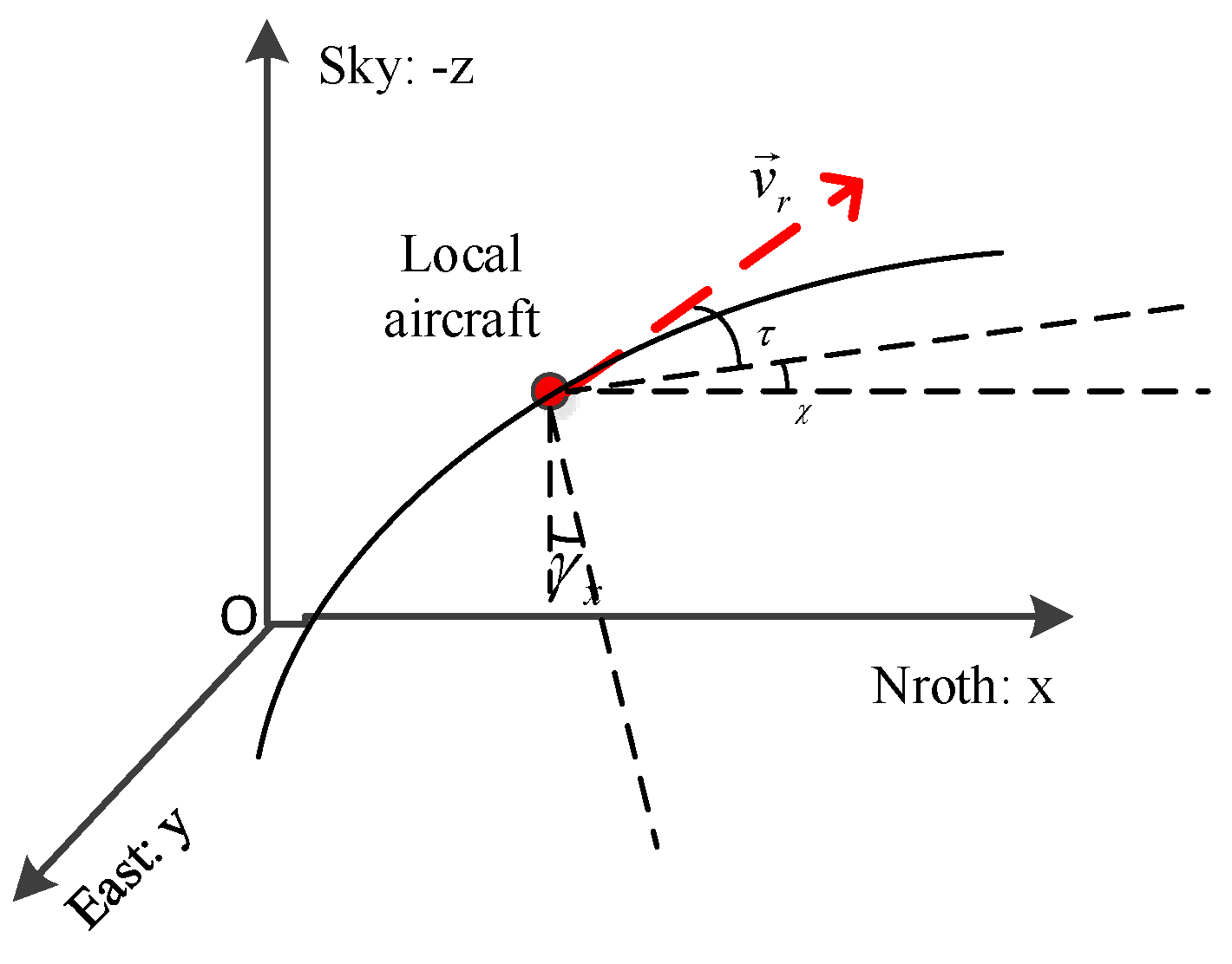
Based on the above assumptions, the force diagram of the aircraft is shown in Figure 1:

where $v$ is the speed of the aircraft, g represents the acceleration of gravity, $n_x$ and $n_f$ indicate the tangential overload and the normal overload, $\tau$, $\chi$ and ${\gamma }_x$ respectively indicate the aircraft’s track inclination angle, track azimuth, and track roll angle. The following formula can be obtained by analyzing the force of the aircraft.

$$\begin{array}{l}mg{n}_x-mg\sin \tau =m\dot{v}\\ mg{n}_f\cos {\gamma }_x-mg\cos \tau =mv\dot{\tau }\\ mg{n}_f\sin {\gamma }_x=mv\cos \tau {\dot{\chi }}_x\end{array}$$

(1)

Transforming the above formula, we can get the dynamic equation of the aircraft as follows:

$$\begin{array}{l}\dot{v}=g(n_x-\sin \tau )\\ \dot{\tau }=\frac{g}{v}(n_f\cos {\gamma }_x-\cos \tau )\\ \dot{\chi }=\frac{g}{v\cos \tau }{n}_f\sin {\gamma }_x\end{array}$$

(2)

In this paper, the movement of the aircraft can be controlled by three quantities of $n_x$, $n_f$ and ${\gamma }_x$. $n_x$ can control the speed of flight, $n_f$ and ${\gamma }_x$ can control the track tilt angle and track azimuth to control flight speed direction.

Based on the above symbol representations, the kinematic equation of the aircraft can be expressed as:

$$\begin{array}{l}\dot{x}=v\cos \tau \cos \chi \\ \dot{y}=v\cos \tau \sin \chi \\ \dot{z}=-v\sin \tau \end{array}$$

(3)

where x, y, and z represent the coordinates of the aircraft in the ground coordinate system (using the North East coordinate system).

2.2. Learning Training Scene Design

Over-the-horizon air confrontation, unlike short-range air confrontation, has powerful missiles, radars, and support for various ground-to-air equipment information, which allows air confrontation to occur at a greater distance. Both parties can speculate through various information support. The opponent’s position is then attacked by the precise guidance of the missile. This paper only studies the maneuvering strategy of over-the-horizon air confrontation, and air confrontation in close range is not considered.

The airspace in which the over-the-horizon air battle is located is assumed as follows (

Table 1. Air confrontation airspace.

Initial Distance/km	End Distance/km	Height/km
65~100	<20	6

): The initial distance between the two sides is 65~100 km; when the distance between the two sides is less than 20 km, it is considered to have entered the close range, and the air battle is over. The height of both sides is 5~7 km.

This paper assumes that the local aircraft has a perception of enemy aircraft during the over-the-horizon air battle. When the enemy aircraft falls within the radar detection range of the local aircraft, enemy information can be obtained more accurately; when the enemy aircraft is not in the radar detection area of the local aircraft, it is assumed that the aircraft can obtain enemy aircraft information through other sources of information in the confrontation system (e.g., ground station radar, airborne early warning aircraft, etc.), but the information obtained by this method has a large error. This assumption is also to ensure that both sides have effective decision-making factors in the one-to-one over-the-horizon air confrontation decision-making process. Otherwise, if the other party’s information is unknown, it is difficult to obtain an effective strategy through the learning algorithm of this paper. This is an area of incomplete information game, which is beyond the scope of this paper.

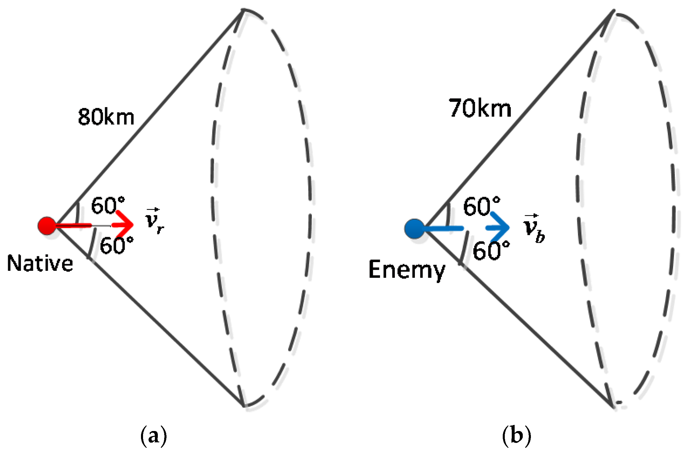
In order to maintain the balance of the two fighters, the performance of both sides is different: the enemy’s missile attack capability is dominant, and the aircraft is dominant in the radar detection range. The specific configuration of the fighter parameters of both parties is shown in

Table 2. Local aircraft performance.

Parameter	Range
Aircraft speed	200 m/s~300 m/s
Radar detection distance	80 km
Radar detection angle	−60°~60°
Missile off-axis launch angle	30°
Missile inescapable cone angle	20°
Missile maximum launch distance	50 km
Missile maximum escape distance	35 km
Missile minimum escape distance	20 km

and

Table 3. Enemy aircraft performance.

Parameter	Range
Aircraft speed	200 m/s~300 m/s
Radar detection distance	70 km
Radar detection angle	−60°~60°
Missile off-axis launch angle	30°
Missile inescapable cone angle	20°
Missile maximum launch distance	55 km
Missile maximum escape distance	40 km
Missile minimum escape distance	25 km

.

According to the configuration in the table, the radar detection area of the unit and the enemy aircraft can be represented by the Figure 2:

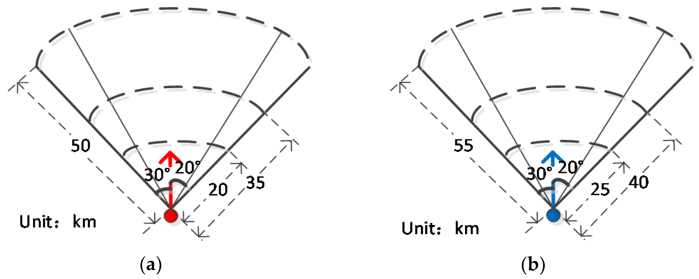
The missile attack zone of both fighters can be expressed in Figure 3:

2.3. Enemy Strategy Design

The enemy aircraft strategy is a very important part of the air confrontation training environment. It determines the fidelity of the over-the-horizon air confrontation environment and also has a great influence on the strategy learned by the algorithm. This paper focuses on the study of air confrontation maneuver strategies with reinforcement learning methods, focusing on the design and improvement of methods, and does not put too much energy into the study of enemy aircraft strategy. Because the air confrontation maneuver strategy learning method studied in this paper is a general method, it is also applicable to training on change in strategy design of the enemy aircraft.

Therefore, this paper identifies enemy strategy as a relatively simple one, which is shown in Figure 4. First, the battlefield situation of the over-the-horizon air confrontation is evaluated based on expert experience. Then, assume that the other party maintains the current state of motion, adopts a method similar to the matrix strategy, and selects the optimal action from the action set as the decision result.

2.4. Reward and Punishment Signal Design

When using the reinforcement learning algorithm to solve practical problems, it is necessary to adjust and optimize the strategy according to the reward and punishment signals fed back by the environment. In the process of constructing the over-the-horizon air confrontation training environment, the reward and punishment signals are mainly considered from two aspects: the detection ability of the aircraft against the enemy aircraft and the threat of the attack on the enemy aircraft.

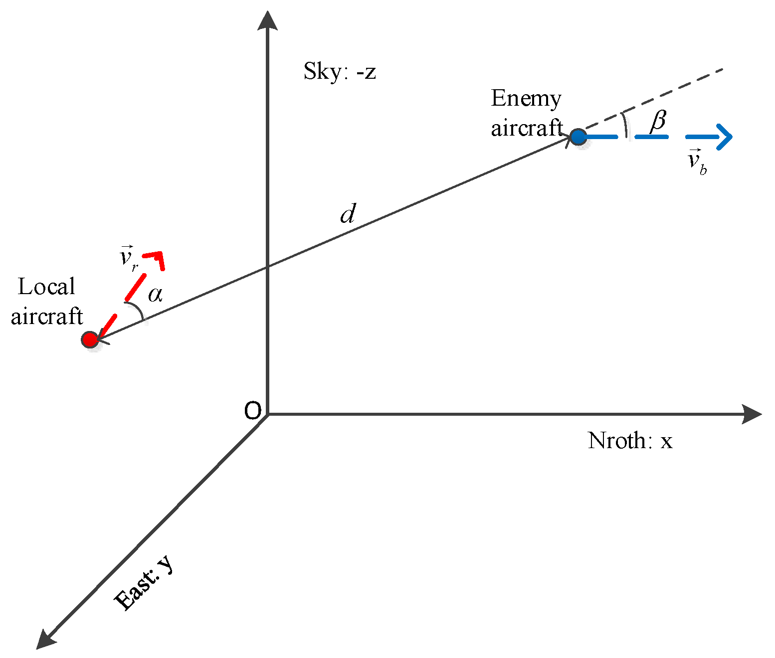
In the process of over-the-horizon air confrontation, the geometric situation of the battlefield is shown in Figure 5.

In Figure 5, ${\overrightarrow{v}}_r$ and ${\overrightarrow{v}}_b$ respectively represent the speed vector of the local aircraft and the speed vector of the enemy aircraft, $\alpha$ indicating the azimuth angle of the enemy aircraft with respect to the local aircraft, $\beta$ indicating the enemy’s entry angle with respect to the local aircraft, and d indicates the distance between the two sides.

2.4.1. Detection Capability

The detection capability of the aircraft to the enemy aircraft is mainly affected by three factors: azimuth $\alpha$, entry angle $\beta$, and distance d between the two sides.

1. Azimuth factor

When the enemy aircraft is located within the maximum detection angle range of the local radar, the aircraft has the ability to detect the enemy aircraft, and thus constructs the azimuth detection advantage:

$$T_{\det \_\alpha }=\{\begin{array}{cc}0,& \left|\alpha \right|>{\alpha }_{FR\max }\\ e^{-\frac{\left|\alpha \right|}{{\alpha }_{FR\max }}},& \left|\alpha \right|\le {\alpha }_{FR\max }\end{array}$$

(4)

${\alpha }_{FR\max }$ is the maximum detection angle of the local fight radar, and FR is the abbreviation of the fight radar.

2. Entry angle factor

This paper assumes that the aircraft airborne radar is a pulse Doppler radar. The characteristics of the radar are: when the target and the local aircraft are head-on, they have strong detection capability, and when the target is on the positive side, the detection capability is poor. The ability to detect a trailing target is less than the ability to detect at the head. Based on this, the advantage of entering the angle detection is constructed as:

$$T_{\det \_\beta }=\{\begin{array}{l}\cos \left(180-\left|\beta \right|\right)\ast e^{-\frac{\pi \ast \left(180-\left|\beta \right|\right)}{180}}\\ ({90}^{\circ }\le \left|\beta \right|<{180}^{\circ })\\ 0.5\cos \left(\left|\beta \right|\right)\ast e^{-\frac{\pi \ast \left|\beta \right|}{180}}\\ (0^{\circ }\le \left|\beta \right|<{90}^{\circ })\end{array}$$

(5)

3. Distance factor

When the enemy aircraft is located within the maximum detection distance of the local radar, the aircraft has the ability to detect the enemy aircraft. Based on this, build a distance detection advantage as:

$$T_{\det \_d}=\{\begin{array}{cc}0,& d>D_{FR\max }\\ e^{-\frac{3\ast d}{D_{FR\max }}},& d\le D_{FR\max }\end{array}$$

(6)

$D_{FR\max }$ is the maximum detection distance of the local radar.

4. Total detection advantage

In an actual air confrontation scenario, the azimuth detection advantage $T_{\det \_\beta }$ and the entry angle detection advantage $T_{\det \_d}$ have a certain coupling, and the overall angle detection advantage is constructed as follows:

$$T_{\det \_ag}={\left(T_{\det \_\alpha }\right)}^{{\gamma }_1}\ast {\left(T_{\det \_\beta }\right)}^{{\gamma }_2}$$

(7)

${\gamma }_1$ and ${\gamma }_2$ are the two parameters that can control the proportion of $T_{\det \_\beta }$ and $T_{\det \_d}$ in the total angular detection advantage. They meet the following conditions: $0\le {\gamma }_1,{\gamma }_2\le 1$ and ${\gamma }_1+{\gamma }_2=1$.

In addition, considering the distance d and the coupling relationship between these angles, the overall detection advantages of constructing the local aircraft to the enemy aircraft are:

$$T_{\det }={\left(T_{\det \_ag}\right)}^{u_1}\ast {\left(T_{\det \_d}\right)}^{u_2}$$

(8)

The role of $u_1$ and $u_2$ is similar to ${\gamma }_1$ and ${\gamma }_2$, and they meet the following conditions: $0\le u_1,u_2\le 1$ and $u_1+u_2=1$.

2.4.2. Attack Threat

The attack threat of the aircraft to the enemy aircraft is mainly affected by three factors: azimuth $\alpha$, energy E and distance d.

1. Azimuth factor

Based on the target azimuth and the performance of the local radar and missile, build an angle threat factor:

$$T_{thr\_\alpha }=\{\begin{array}{cc}0& \alpha >{\alpha }_R\\ 0.3(1-\frac{\left|\alpha \right|-{\alpha }_M}{{\alpha }_R-{\alpha }_M})& {\alpha }_M\le \left|\alpha \right|\le {\alpha }_R\\ 0.8-\frac{\left|\alpha \right|-{\alpha }_{Mk}}{2({\alpha }_M-{\alpha }_{Mk})}& {\alpha }_{Mk}\le \left|\alpha \right|<{\alpha }_M\\ 1-\frac{\left|\alpha \right|}{5{\alpha }_{Mk}}& 0\le \left|\alpha \right|<{\alpha }_{Mk}\end{array}$$

(9)

${\alpha }_R$ is the maximum search angle of the local radar, ${\alpha }_M$ is the maximum attack angle of the local missile, ${\alpha }_{Mk}$ is the maximum angle of the non-escape zone of the local missile.

2. Energy factor

In the air confrontation process, the higher the energy of the fighter, the stronger the attacking ability of the launched missile, and the greater the threat to the enemy aircraft. The energy here is mainly composed of kinetic energy, according to the kinetic energy formula, which is simplified as follows:

$$E=\frac{v^2}{2g}$$

(10)

v is the speed of the local aircraft, g is the gravitational acceleration, and weight can be ignored considering the particle model.

Based on this, build the native energy threat factor:

$$T_{thr\_E}=\{\begin{array}{ll}1,& \frac{E}{E_T}\ge 2\\ {0.5}^{2-\frac{E}{E_T}},& 0.5\le \frac{E}{E_T}<2\\ \frac{E}{2E_T},& \frac{E}{E_T}<0.5\end{array}$$

(11)

E is the energy of the aircraft and $E_T$ is the enemy aircraft’s energy.

3. Distance factor

The distance threat factor is constructed based on the distance between the enemy and the enemy and the performance of the local radar and missile:

$$T_{thr\_d}=\{\begin{array}{cc}0& d\ge D_R\\ 0.5e^{-\frac{d-D_{M\max }}{D_R-D_{M\max }}}& D_{M\max }\le d<D_R\\ 2^{-\frac{d-D_{Mk\max }}{D_{M\max }-D_{Mk\max }}}& D_{Mk\max }\le d<D_{M\max }\\ 1& D_{Mk\min }\le d<D_{Mk\max }\\ 2^{-\frac{d-D_{Mk\min }}{10-D_{Mk\min }}}& 10\le d<D_{Mk\min }\\ 0& d<10\end{array}$$

(12)

$D_R$ is the maximum search distance of the local radar, $D_{M\max }$ is the maximum attack distance of the local missile, $D_{Mk\max }$ is the maximum inescapable distance of the local missile, and $D_{Mk\min }$ is the minimum inescapable distance of the local missile.

4. Total attack threat

Considering that the distance factor and the angle factor have a certain coupling relationship, the total attack threat of the aircraft to the enemy aircraft is:

$$T_{thr}=k_1\ast {\left(T_{thr\_\alpha }\right)}^{{\eta }_1}\ast {\left(T_{thr\_d}\right)}^{{\eta }_2}+k_2\ast T_{thr\_E}$$

(13)

$k_1$, $k_2$, ${\eta }_1$ and ${\eta }_2$ are control parameters, and they meet the following conditions:

$0\le {\eta }_1,{\eta }_2\le 1$, ${\eta }_1+{\eta }_2=1$, $0\le k_1,k_2\le 1$ and $k_1+k_2=1$.

2.4.3. Reward and Punishment Signal Synthesis

According to the above-mentioned advantages of the detection capability of the enemy aircraft and the threat of attack, the total threat of constructing the local aircraft is:

$$T={\left(T_{\det }\right)}^{{\gamma }_1}\ast {\left(T_{thr}\right)}^{{\gamma }_2}$$

(14)

The two parameters ${\gamma }_1,{\gamma }_2$ are the index of the local aircraft detection capability and the attack threat, which determine the importance ratio of the two in the reward and punishment function. These two values can be obtained empirically.

In the same way, the enemy’s threat to the local aircraft can be found, which is defined as $T_t$, and the reward and punishment signals are designed accordingly:

$$R=T-T_t$$

(15)

R is the relative threat value of the enemy aircraft to the enemy aircraft. When the local threat is greater than the enemy aircraft threat, the reward is positive, otherwise it is negative.

3. Markov Decision Process Modeling

The Markov decision process [14] can be represented by a six-tuple $\langle S,A,P,R,\gamma ,V\rangle$. The aircraft constructed in this paper is a model; there is no random item. The element P can be omitted here. At the same time, the reward and punishment function R has also been designed before. Therefore, in this section, only state space S, action space A, discount factor $\gamma$, and objective function V of MDP [15] need to be determined.

3.1. Air Confrontation State Space

According to the battlefield geometry map, the battlefield situation can be expressed in 9 quantities: $\alpha$, $\beta$, d, $v_r$, $v_b$, ${\tau }_r$, ${\tau }_b$, ${\gamma }_r$, ${\gamma }_b$. They respectively indicate the azimuth angle of the enemy aircraft relative to the aircraft, the angle of entry of the enemy aircraft with respect to the aircraft, the distance between the two sides, the speed of the aircraft, the speed of the enemy aircraft, the inclination angle of the local aircraft, the inclination angle of the enemy aircraft track, and the present aircraft track roll angle and enemy aircraft track roll angle. Considering whether the enemy aircraft is located in the local radar detection range, the accuracy of the enemy aircraft information obtained by the aircraft is not the same, so a confidence factor c (confidence) is added to indicate the accuracy of the enemy information. The larger c, the more accurate the information. It meets the conditions: $0\le c\le 1$.

The air confrontation state can be represented by a 10-dimensional vector:

$$s=\left(\alpha ,\beta ,d,v_r,v_b,{\tau }_r,{\tau }_b,{\gamma }_r,{\gamma }_b,c\right)$$

(16)

3.2. Maneuvering Decision Action Space

In the over-the-horizon air confrontation maneuver decision problem, establishing a reasonable maneuver library is the key to air confrontation intelligent decision-making [16]. Generally, air confrontation maneuver library design is divided into two types: One is the “25 typical tactical actions” based on the classic tactics of pilots in air confrontation, including straight-flat, fixed-height, slow-speed Yo-Yo; The other is a “basic manipulation action library” based on common air confrontation control methods, including maximum acceleration/deceleration, maximum load climb/deep, maximum load left/right turn, stable flight, etc.

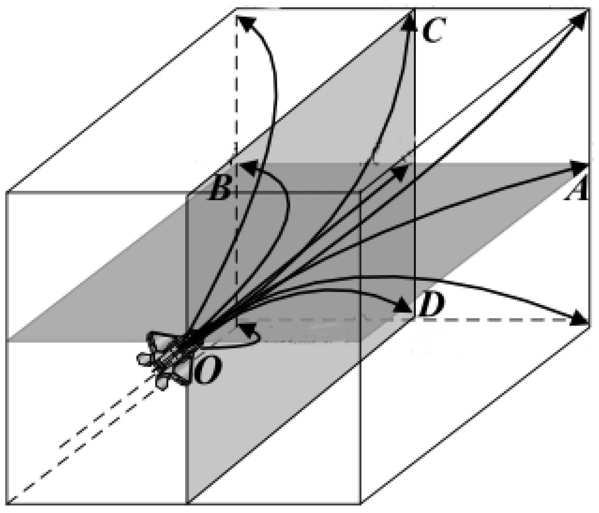
As shown in Figure 6, the air confrontation maneuver library is built according to the “Basic Manipulation Action Library”, including nine maneuver directions: left climb, climb, right climb, horizontal left turn, horizontal forward fly, horizontal right turn, left dive, dive, and right dive. In this paper, assuming that both sides move on a horizontal plane, there are only three optional actions: horizontal left turn, horizontal forward fly, and horizontal right turn. In these three directions, it can be divided according to the change of speed: increase, hold and decrease. Therefore, there are a total of nine optional maneuvers, that is $\left|A\right|=9$.

According to the previous description of the aircraft model, the motion of the aircraft is mainly controlled by the three quantities of $n_x$, $n_f$ and ${\gamma }_x$, which respectively represent tangential overload, normal overload, and track roll angle. $n_x$ is used to control speed, $n_f$ and ${\gamma }_x$ are used to control speed direction. According to these three quantities, action space A can be defined as follows (

Table 4. Action collection.

Action	${\mathit{\gamma }}_{\mathit{x}}$, ${\mathit{n}}_{\mathit{x}}$, ${\mathit{n}}_{\mathit{f}}$	Speed Direction	Speed Size
a1	(−1, −1, 0)	turn left horizontally	Decrease
a2	(−1, 0, 0)	turn left horizontally	Maintain
a3	(−1, 1, 0)	turn left horizontally	Increase
a4	(0, −1, 0)	fly forward horizontally	Decrease
a5	(0, 0, 0)	fly forward horizontally	Maintain
a6	(0, 1, 0)	fly forward horizontally	Increase
a7	(1, −1, 0)	turn right horizontally	Decrease
a8	(1, 0, 0)	turn right horizontally	Maintain
a9	(1, 1, 0)	turn right horizontally	Increase

):

3.3. Discount Factor and Objective Function

In the application of reinforcement learning, the discount factor has two main functions: (1) the reward and punishment signal decays with time, indicating that it is less important in the far-away time; (2) it can prevent accumulation due to the excessive length of the episode. The reward is too large, and the cumulative reward value can be bounded by the attenuation factor. It is often set to 0.9, so this article also follows this setting.

The optimization objective function uses a state limited discount type objective function, in which it estimates the function V only based on the reward value of the state of the next n moments at the current moment:

$$V^{\pi }({\mathrm{s}}_t)={\mathrm{E}}_{\pi }(\mathrm{R}({\mathrm{s}}_t))={\mathrm{E}}_{\pi }({\displaystyle \sum _{k=0}^{n-1}{\gamma }^k{r}_{t+k}})$$

(17)

4. Heuristic Q-Network

In view of the over-the-horizon air confrontation maneuver decision problem, this paper adopts an indirect strategy, which is to generate a strategy by obtaining a behavior value function $Q(s,a)$. For the decision-making of maneuvering, this paper also uses the Q-Network algorithm [17].

The reinforcement learning algorithm [18] solves the strategy by interacting with the environment, which is a process of sensing the unknown environment and learning related knowledge. According to the utilization of current knowledge, the learning process of the algorithm can be divided into two kinds of behaviors: exploration and exploitation. Exploitation is based on the currently learned strategy, which enables the agent to obtain many rewards. In addition, exploration is to try new actions in order to find better strategies to get more rewards in the future. In the process of solving practical problems, it is necessary to find a suitable compromise between exploitation and exploration, which will make the algorithm more efficient.

The often-used exploitation strategy is a strategy, which can be expressed as follows (Algorithm 1):

Algorithm 1.$\epsilon -greedy$ strategy.

Input: control parameter $\epsilon$ Process:  1: if random() < $\epsilon$  2: action$\leftarrow$random from set A  3: else  4: action$\leftarrow$$\underset{a}{\arg \max }Q(s,a)$  5: end if

Under the exploration strategy of $\epsilon -greedy$, the algorithm can converge to an effective strategy through repeated training, but this way of exploring is very inefficient, because in the process of exploration, it randomly selects an action from the action set each time. The randomly selected actions are often useless, which leads to a lot of invalid exploration.

For the over-the-horizon air confrontation maneuver decision problem, we can introduce and use expert knowledge as a heuristic signal to guide the exploration process. This algorithm is called Heuristic Q-Network, which is shown as follows(Algorithm 2):

Algorithm 2. The exploration process of heuristic Q-Network.

Input: control parameter $\epsilon$ Process:  1: if random() < $\epsilon$  2: action$\leftarrow$ heuristic_strategy(s)  3: else  4: action$\leftarrow$$\underset{a}{\arg \max }Q(s,a)$  5: end if

5. Air Confrontation Strategy Learning

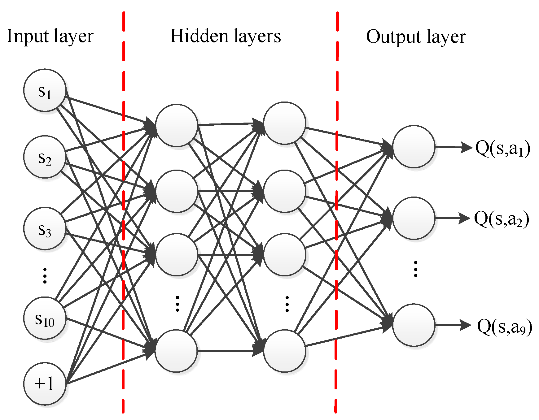
For the two-dimensional over-the-horizon air confrontation problem, according to the previous MDP model, heuristic Q-Network is used. The Q-Network structure used in this paper is an MLP with two hidden layers, which is shown in Figure 7. Its input is the air confrontation states, and the output is the behavior value function $Q(s,a_i)$ corresponding to nine maneuvers. The number of hidden layer nodes can be selected by contrast experiment. The number of nodes in the network hidden layer is determined by experiments—64 in the first hidden layer and 128 in the second layer.

Using the heuristic + random exploration method, the score curve of the Q-Network training process is shown in Figure 8.

The blue curve indicates the exploration strategy of $\epsilon -greedy$, and the orange curve indicates the heuristic + random exploration strategy. It can be slightly seen that the heuristic search strategy can obtain a higher expected score, which further validates the effectiveness of the heuristic Q-Network.

6. Simulation Result Verification

The heuristic Q-Network learning strategy is used in air confrontation simulation, and several typical air confrontation cases are selected for analysis. According to the initial air confrontation situation, the initial state of the local aircraft can be divided into: advantage, balance and disadvantages.

• Advantage

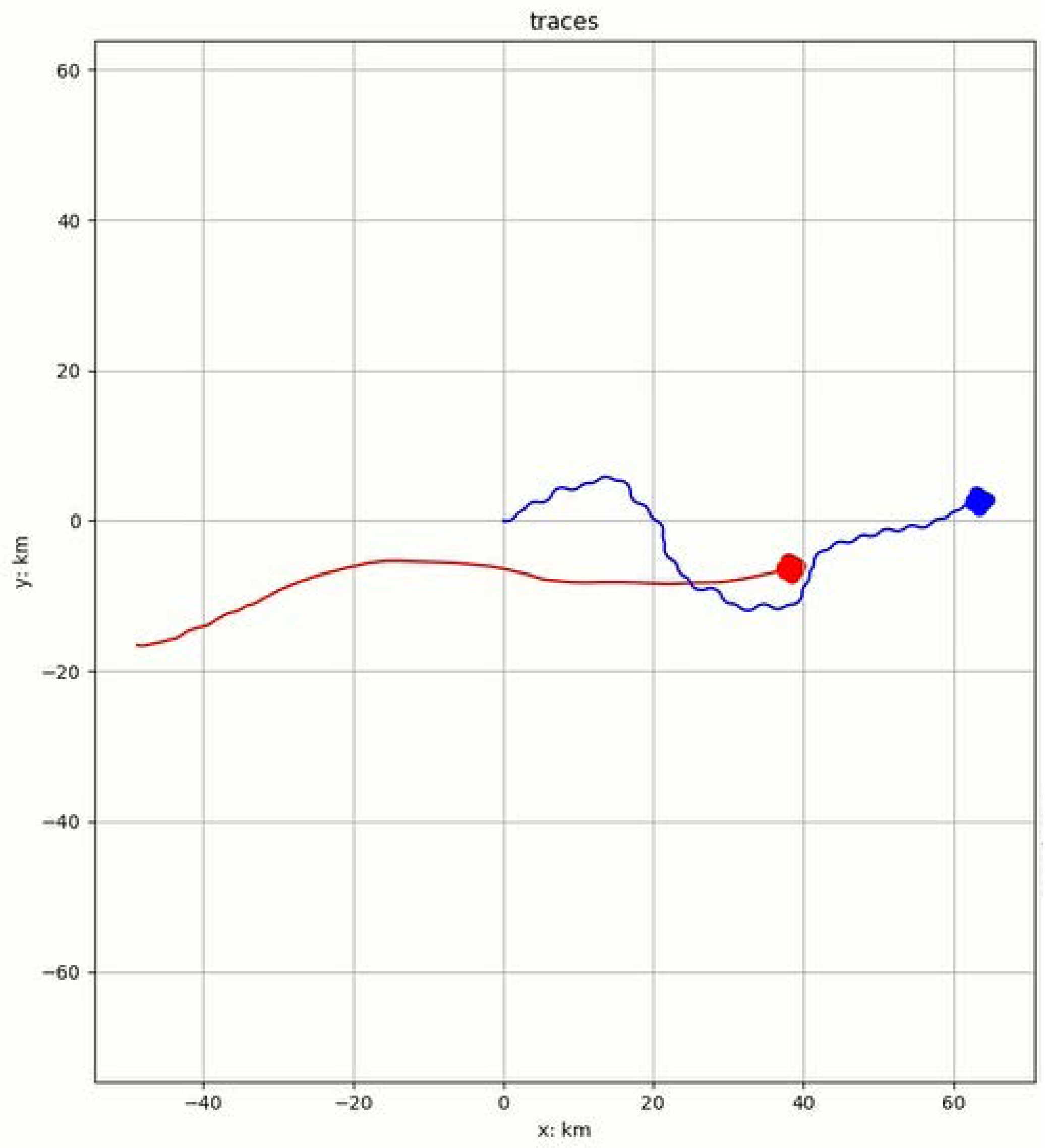
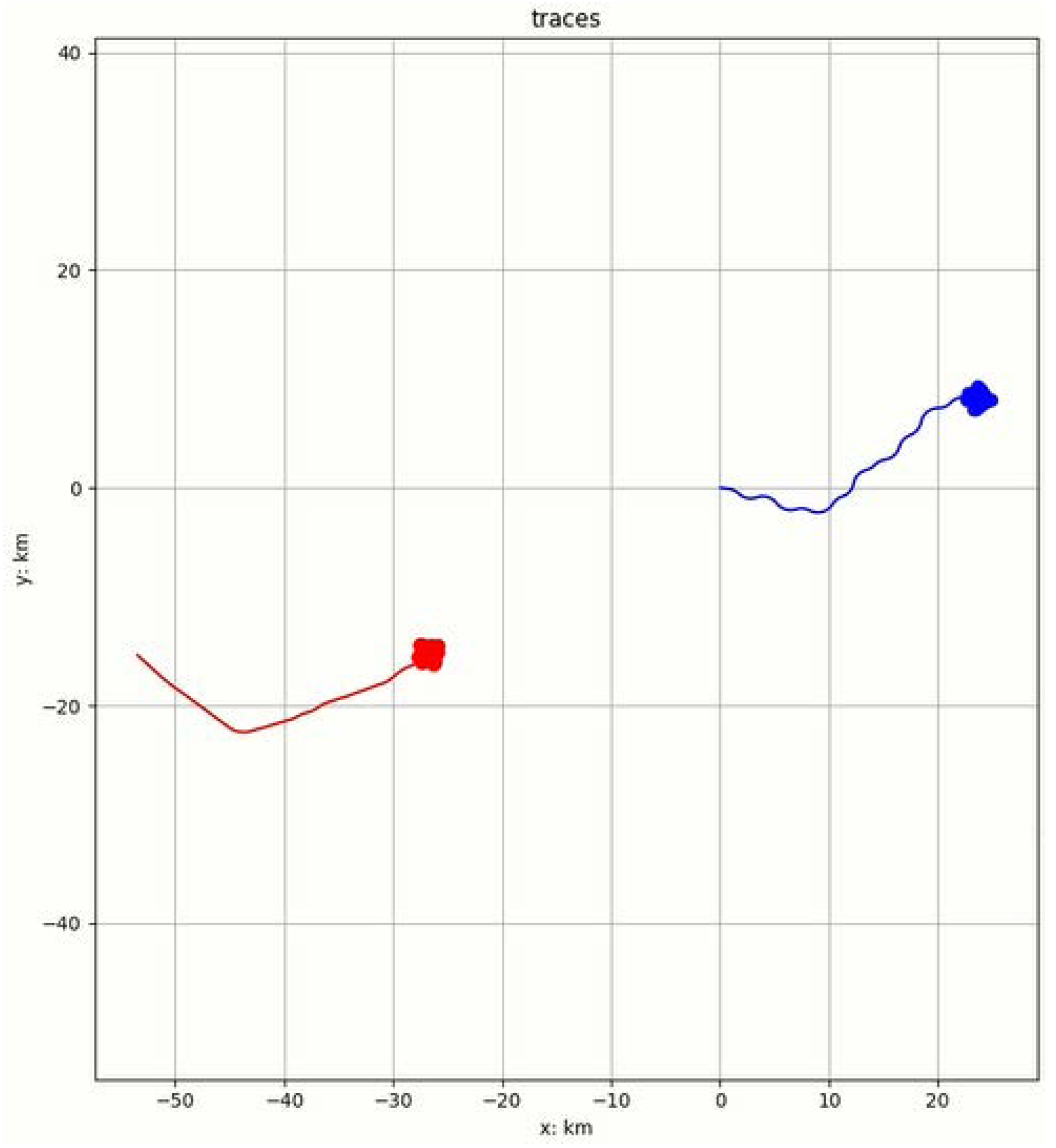
Figure 9 shows the air confrontation process when the unit is initially in an advantageous position, where the unit is indicated in red, and the enemy aircraft is shown in blue.

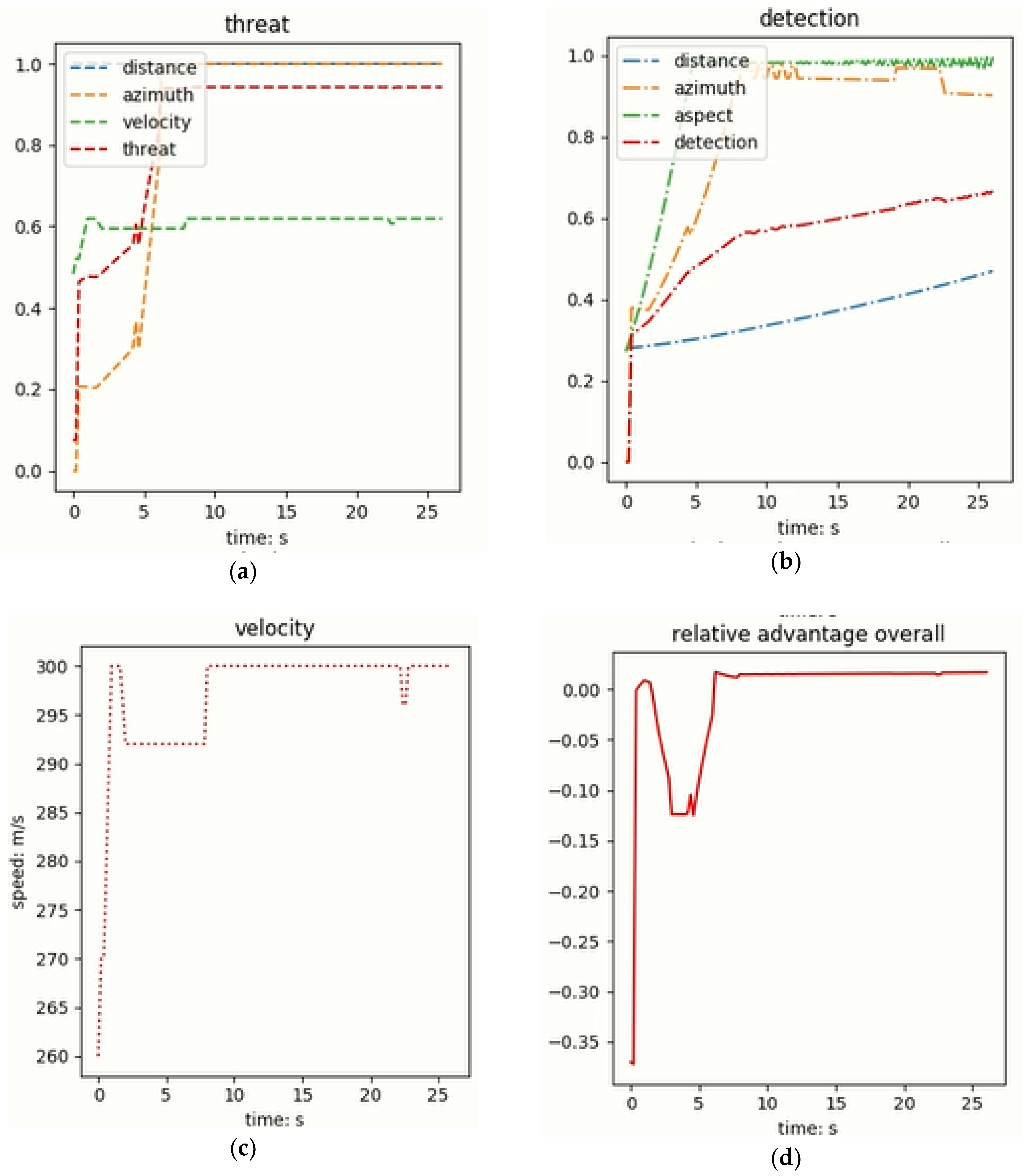
Figure 10 records the changes in the relevant data of the aircraft during the above air confrontation process, including: the threat capability (Figure 10a), detection capability (Figure 10b), speed (Figure 10c) and relative advantage of the aircraft to the enemy aircraft (Figure 10d).

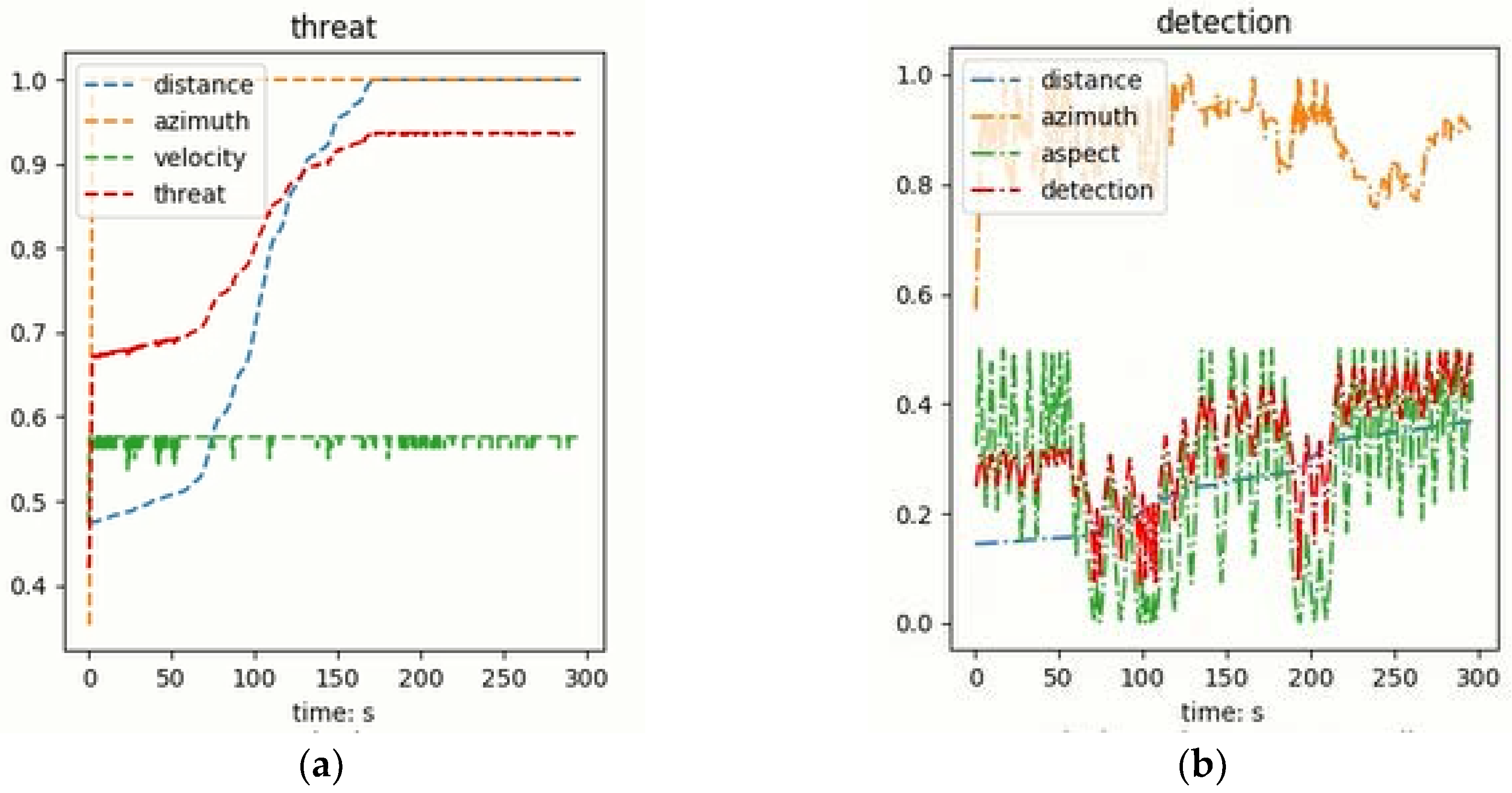
As can be seen from Figure 10, when the local aircraft is at an advantage, the local aircraft further increases its advantages from several aspects. In Figure 10a, the local aircraft increases the azimuth threat advantage of the enemy aircraft by changing its own heading, changing the speed to increase the energy advantage of the enemy aircraft, and reducing the distance between the two sides to increase the distance threat advantage. Through these three factors, the overall threat capability of the aircraft to the enemy aircraft is greatly enhanced. In Figure 10b, by changing the heading to increase the azimuth detection advantage and the entry angle detection advantage of the enemy aircraft, by narrowing the distance between the two sides to increase the distance detection advantage, the three factors can improve the comprehensive detection capability of the aircraft to the enemy aircraft. As shown in Figure 10d, the overall relative advantage of the aircraft against the enemy aircraft is on the rise. The fluctuation is due to the change of the enemy’s entry angle, which causes the oscillation of the entry angle. This factor is difficult to control for the aircraft. The heading has a greater impact, and the local aircraft mainly enhances the angle advantage by changing the azimuth.

• Balance

Figure 11 shows the air confrontation process when the unit is initially in balance. The unit is indicated in red and the enemy aircraft is shown in blue.

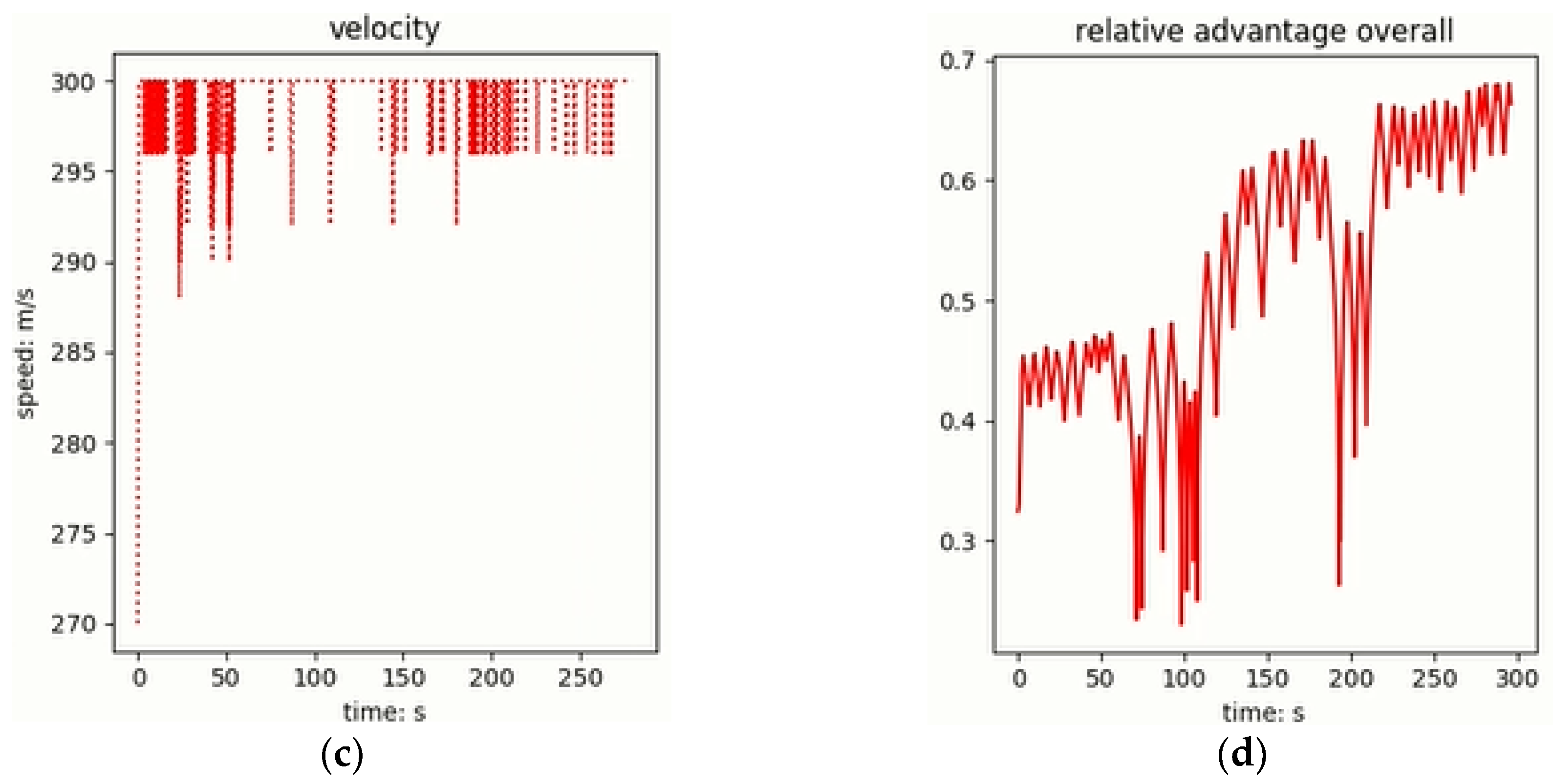
Figure 12 shows the data changes of the local aircraft during the above air confrontation. Figure 12a shows changes in threat capabilities and comprehensive threat capabilities in all aspects, Figure 12b shows changes in detection capabilities and comprehensive detection capabilities, and Figure 12c shows changes in local speed. Figure 12d shows the overall advantage of the local aircraft relative to the enemy aircraft changes; from the figure, it can be seen that the initial relative advantage is zero, and the local aircraft, through a series of maneuvering decisions, can improve the relative advantage, so that it is in a higher position.

• Disadvantage

Figure 13 shows the air confrontation process when the unit is initially at a disadvantage. The unit is indicated in red and the enemy aircraft is shown in blue.

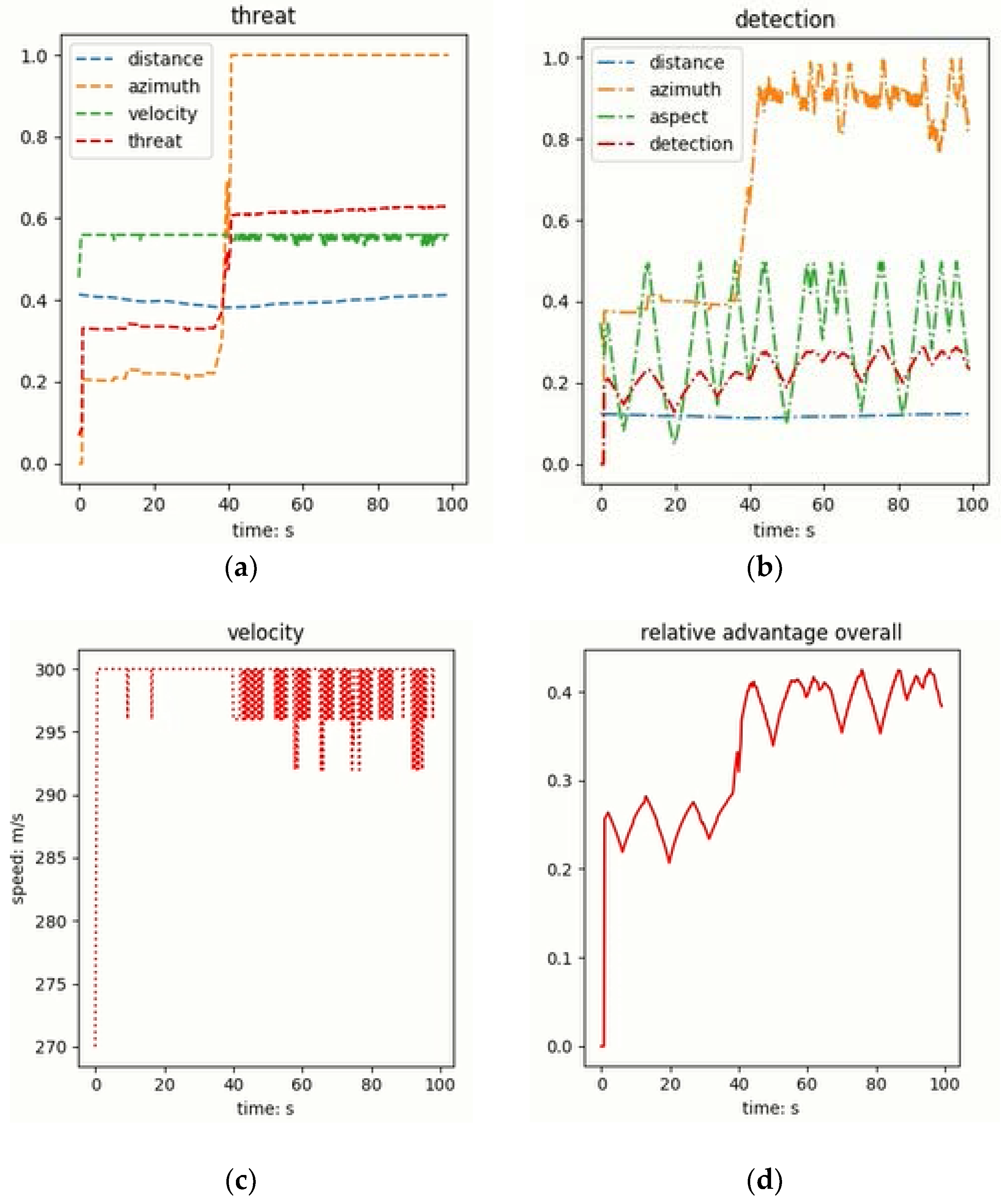
Figure 14 shows the data changes of the local aircraft during the above air confrontation. Figure 14a,b respectively show the changes in the threat capability and detection capability of the local aircraft to the enemy aircraft. Although there are some fluctuations, the overall trend is correct. And Figure 14c shows changes in local speed. It can also be seen from Figure 14d that the overall advantage of the local aircraft relative to the enemy aircraft increases from the initial negative value to a positive value, and there are some oscillations in the middle, but in the end, it can be stably maintained at a positive value, that is, in an advantageous position.

• Other cases

In order to further demonstrate the air confrontation maneuver strategy learned through training, this paper presents a two-dimensional air confrontation simulation process under different initial conditions. As shown in Figure 15, the local aircraft can make better maneuvering decisions in the battle between the two sides and gain a greater advantage in confrontation.

7. Conclusions

In the process of over-the-horizon air confrontation, automated and reasonable maneuver decision-making is the premise of independent decision-making such as weapon attack, sensor use, electronic countermeasures, etc. It is accompanied by the entire air confrontation process and is an extremely important part of the automated air confrontation system/air confrontation assisted decision-making. This paper mainly studies the maneuvering decision-making method of intelligent fighters in this environment based on the single-to-single air confrontation confrontation in super-horizon air confrontation. The maneuvering decision algorithm based on reinforcement learning realizes the self-learning of the air confrontation maneuver strategy, and finally helps the fighters make reasonable maneuver decisions independently under different air confrontation situations. However, due to time and condition constraints, this work needs further research. For example, height information can be added to make the air confrontation confrontation more realistic, and the air confrontation training environment and enemy aircraft maneuver strategy need to be further improved.

References

- Ehtamo, H.; Raivio, T. On Applied Nonlinear and Bi-level Programming or Pursuit-Evasion Games. J. Optim. Theory Appl. 2001, 108, 65–96. [Google Scholar] [CrossRef]
- Fu, L.; Xie, F.; Wang, D.; Meng, G. The Overview for UAV Air-combat Decision Method. In Proceedings of the Chinese Control and Decision Conference, Changsha, China, 31 May–2 June 2014; pp. 3380–3384. [Google Scholar]
- Austin, F.; Carbone, G.; Hinz, H.; Lewis, M.; Falco, M. Game Theory for Automated Maneuvering During Air-to-Air Com-bat. J. Guidance 1990, 13, 1143–1147. [Google Scholar] [CrossRef]
- McManus, J.W.; Chappell, A.R.; Arbuckle, P.D. Situation Assessment in the Paladin Tactical Decision Generation System. In Proceedings of the Air Vehicle Mission Control and Management, CA:AGARD Conference, Paris, France, 1 March 1992; pp. 1–10. [Google Scholar]
- Virtanen, K.; Raivio, T.; Hamalainen, R.P. Modeling pilot’s sequential maneuvering decisions by a multistage influence diagram. J. Guid. Control. Dyn. 2004, 27, 665–677. [Google Scholar] [CrossRef]
- Ernest, N.; Cohen, K.; Kivelevitch, E.; Schumacher, C.; Casbeer, D. Genetic fuzzy trees and their application towards autonomous training and control of a squadron of unmanned combat aerial vehicles. Unmanned Syst. 2015, 03, 185–204. [Google Scholar] [CrossRef]
- Ernest, N.; Carroll, D. Genetic fuzzy based artificial intelligence for unmanned combat aerial vehicle control in simulated air combat missions. J. Déf. Manag. 2016, 06. [Google Scholar] [CrossRef]
- Krishna Kumar, K.; Kaneshige, J.; Satyadas, A. Challenging Aerospace Problems for Intelligent Systems. In Proceedings of the Von Karman Lecture Series on Intelligent Systems for Aeronautics, Brussels, Belgium, 13–17 May 2002; pp. 1–15. [Google Scholar]
- Krishnakumar, K.; Kaneshige, J. Artificial Immune System Approach for Air Combat Maneuvering. Proc. SPIE Intell. Comput. Theor. Appl. V 2007, 6560, 1–12. [Google Scholar]
- Schvaneveldt, R.W.; Goldsmith, T.E.; Benson, A.E.; Waag, W.L. Neural Network Models of Air Combat Maneuvering; New Mexico State University: Las Cruces, NM, USA, 1992. [Google Scholar]
- McGrew, J.S.; How, J.P.; Williams, B.; Roy, N. Air Combat Strategy using Approximate Dynamic Programming. J. Guidance Control Dyn. 2010, 33, 1641–1654. [Google Scholar] [CrossRef]
- Yang, X.; Wang, X.H.; Shen, G.X.; Wen, C.Y. Modeling and Simulation Research of Six-Degree-of-Freedom Fighter. J. Syst. Simul. 2000, 12, 210–213. [Google Scholar]
- Lachner, R.; Breitner, M.H.; Pesch, H.J. Three-dimensional air combat: Numerical solution of complex differential games. New Trends Dyn. Games Appl. 1995, 165–190. [Google Scholar] [CrossRef]
- Howard, R.A. Dynamic Programming and Markov Process. Math. Gaz. 1960, 3, 120. [Google Scholar]
- Li, S.; Liu, G.; Wu, J. A Self-learning Terrain-following Method for Aircrafts. In Proceedings of the China Control Conference, Dalian, China, 26–28 July 2017; pp. 3437–3442. [Google Scholar]
- Dong, X.L.; Tong, Z.X.; Wang, B.N. Design of the BVRAC Maneuver Library and Visualization of Movements. Flight Mech. 2005, 23, 90–93. [Google Scholar]
- Touzet, C.F. Neural networks and Q-learning for robotics. In Proceedings of the IJCNN’99 (International Joint Conference (IEEE INNS) on Neural Networks), Washington, DC, USA, 10–16 July 1999. [Google Scholar]
- Sutton, R.S.; Barto, A.G. Reinforcement Learning: An Introduction; MIT Press: Cambridge, UK, 1998. [Google Scholar]
© 2018 by the authors. Licensee MDPI, Basel, Switzerland. This article is an open access article distributed under the terms and conditions of the Creative Commons Attribution (CC BY) license (http://creativecommons.org/licenses/by/4.0/).