Fully Quaternion-Valued Adaptive Beamforming Based on Crossed-Dipole Arrays

Abstract

Based on crossed-dipole antenna arrays, quaternion-valued data models have been developed for both direction of arrival estimation and beamforming in the past. However, for almost all the models, and especially for adaptive beamforming, the desired signal is still complex-valued as in the quaternion-valued Capon beamformer. Since the complex-valued desired signal only has two components, while there are four components in a quaternion, only two components of the quaternion-valued beamformer output are used and the remaining two are simply discarded, leading to significant redundancy in its implementation. In this work, we consider a quaternion-valued desired signal and develop a fully quaternion-valued Capon beamformer which has a better performance and a much lower complexity. Furthermore, based on this full quaternion model, the robust beamforming problem is also studied in the presence of steering vector errors and a worst-case-based robust beamformer is developed. The performance of the proposed methods is verified by computer simulations.

1. Introduction

Electromagnetic (EM) vector sensor arrays can track the direction of arrival (DOA) of impinging signals as well as their polarization. A crossed-dipole sensor array—firstly introduced in [1] for adaptive beamforming—works by processing the received signals with a long polarization vector. Based on such a model, the beamforming problem was studied in detail in terms of output signal-to-interference-plus-noise ratio (SINR) [2]. In [3,4], further detailed analysis was performed showing that the output SINR is affected by DOA and polarization differences.

Since there are four components for each vector sensor output in a crossed-dipole array, a quaternion model instead of long vectors has been adopted in the past for both adaptive beamforming and direction of arrival estimation [5,6,7,8,9,10,11,12]. In [13], the well-known Capon beamformer was extended to the quaternion domain and a quaternion-valued Capon (Q-Capon) beamformer was proposed with the corresponding optimum solution derived.

However, in most of the beamforming studies, the signal of interest (SOI) is still complex-valued; i.e., with only two components: in-phase (I) and quadrature (Q). Since the output of a quaternion-valued beamformer is also quaternion-valued, only two components of the quaternion are used to recover the SOI, which leads to redundancy in both calculation and data storage. However, with the development of quaternion-valued communications [14,15,16], it is very likely that in the future we will have quaternion-valued signals as the SOI, where two traditional complex-valued signals with different polarisations arrive at the antenna array with the same DOA. In such a case, a full quaternion-valued array model is needed to compactly represent the four-component desired signal and also make sure the four components of the quaternion-valued output of the beamformer are fully utilised. In this work, we develop such a model and propose a new quaternion-valued Capon beamformer, where both its input and output are quaternion-valued.

Based on the proposed full quaternion model, we further study the robust adaptive beamforming problem in the presence of steering vector errors. In the past, many methods have been proposed to improve the robustness of an adaptive beamformer, such as diagonal loading [17,18] and those based on the optimization of worst-case performance [19,20]. In [11], the worst-case-based method is extended to the quaternion-valued case for crossed-dipole arrays; however, it is not a full quaternion model, since the desired signal is still complex-valued. In this work, we extend the worst-case optimisation approach to the full quaternion model and a worst-case-based full-quaternion robust adaptive beamforming method is proposed.

This paper is structured as follows. The full quaternion-valued array model is introduced in Section 2, and the proposed full quaternion-valued Capon beamformer is developed in Section 3. The robust beamforming problem is studied in Section 4 based on the worst-case optimisation approach. Simulation results are presented in Section 5, and conclusions are drawn in Section 6.

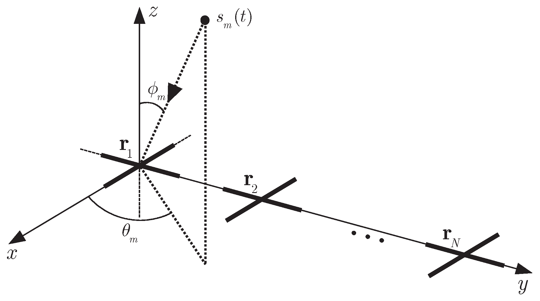
2. Quaternion Model for Crossed-Dipole Array

2.1. Basics of Quaternion

Quaternion was introduced by W. R. Hamilton [21]. A quaternion is constructed by four components, with one real part and three imaginary parts, defined as

$$q=q_a+i{q}_b+j{q}_c+k{q}_d$$

(1)

where i, j, k are three basic imaginary units. The multiplication principle among such units is

$$i^2=j^2=k^2=ijk=-1,$$

(2)

and

$$ij=-ji=k,ki=-ik=j,jk=-kj=i$$

(3)

The conjugate $q^{*}$ of q is $q^{*}=q_a-i{q}_b-j{q}_c-k{q}_d$.

Note that the multiplication of quaternions is generally non-commutative: for $q_1,q_2\in \mathbb{H}$, $q_1{q}_2\ne q_2{q}_1$, where $\mathbb{H}$ represents the quaternion domain. However, if one of the factors (e.g., $q_0$) is real, then we have $q_0{q}_1=q_1{q}_0$.

2.1.1. Quaternion Vector and Matrix

Quaternion vectors and matrices are quite different from real and complex ones. For quaternion vectors, the space can be denoted by two different bases—left-spanned and right-spanned—given by

$$spa{n}_L\{u_1,u_2,...u_M\},spa{n}_R\{u_1,u_2,...u_M\}.$$

(4)

Here we use ${\mathit{q}}_L$ to denote the left linear combination case and ${\mathit{q}}_R$ to denote the right linear combination case. Note that $q={\mathit{q}}_L={\mathit{q}}_R$,

$$\begin{array}{c}{\mathit{q}}_L={\displaystyle \sum _{m=1}^M}{\tau }_m{\mathbf{u}}_m\\ {\mathit{q}}_R={\displaystyle \sum _{m=1}^M}{\mathbf{u}}_m{\gamma }_m\end{array}$$

(5)

where ${\tau }_m,{\gamma }_m\in \mathbb{H}$, for $m=1,2,...,M$.

Similarly, the eigendecomposition operation for quaternion matrices also differs from real and complex ones. We can also define the left eigendecomposition ${\mathit{Q}}_L$ and right eigendecomposition ${\mathit{Q}}_R$ for a Hermitian matrix $\mathit{Q}\in {\mathbb{H}}^{N\times N}$, ($\mathit{Q}={\mathit{Q}}^{\mathrm{H}}$, where ${\left\{\right\}}^{\mathrm{H}}$ is the Hermitian transpose, a combination of the quaternion-valued conjugate and transpose operations)

$$\begin{array}{c}{\mathit{Q}}_L={\displaystyle \sum _{n=1}^N}{\alpha }_n{\mathit{u}}_n{\mathit{u}}_n^{\mathrm{H}}\\ {\mathit{Q}}_R={\displaystyle \sum _{n=1}^N}{\mathit{u}}_n{\mathit{u}}_n^{\mathrm{H}}{\mathbf{\beta }}_n\end{array}$$

(6)

where $\alpha$ and $\mathbf{\beta }$ are the left and right eigenvalues [5,22,23]. In this paper, only right-spanned spaces and left eigendecomposition are employed.

2.1.2. The Gradient for a Quaternion Function

Let $l\left(\mathbf{w}\right)$ be a scalar function of the quaternion-valued vector $\mathbf{w}\in {\mathbb{H}}^{N\times 1}$, with $\mathbf{w}={[w_1...w_n...w_N]}^{\mathrm{T}}$, and $w_n=w_{na}+w_{nb}i+w_{nc}j+w_{nd}k$.

Its gradient with respect to $\mathbf{w}$ is defined by [24]

$${\nabla }_{\mathbf{w}}l={[{\nabla }_{w_1}l...{\nabla }_{w_n}l...{\nabla }_{w_N}l]}^{\mathrm{T}}$$

(7)

where

$${\nabla }_{w_n}l=\frac{1}{4}({\nabla }_{w_{na}}l+{\nabla }_{w_{nb}}li+{\nabla }_{w_{nc}}lj+{\nabla }_{w_{nd}}lk)$$

(8)

$${\nabla }_{w_n^{*}}l=\frac{1}{4}({\nabla }_{w_{na}}l-{\nabla }_{w_{nb}}li-{\nabla }_{w_{nc}}lj-{\nabla }_{w_{nd}}lk)$$

(9)

2.2. Model for Crossed-Dipole Array

A quaternion number $q=q_a+i{q}_b+j{q}_c+k{q}_d$ can be conveniently expressed as a combination of two complex numbers $c_1=q_a+j{q}_c$ and $c_2=q_b+j{q}_d$, as follows

$$q=c_1+i{c}_2=(q_a+j{q}_c)+i(q_b+j{q}_d)=q_a+i{q}_b+j{q}_c+k{q}_d$$

(10)

We will use this form later to represent our quaternion-valued signal of interest.

Consider a uniform linear array (ULA) with N crossed-dipole sensors, as shown in Figure 1, where the adjacent vector sensor spacing d equals half wavelength, and the two components of each crossed-dipole are parallel to x- and y-axes, respectively. A quaternion-valued narrowband signal $s_0\left(t\right)$ impinges upon the vector sensor array among other M uncorrelated quaternion-valued interfering signals ${\left\{s_m\left(t\right)\right\}}_{m=1}^M$, with background noise $n\left(t\right)$. $s_0\left(t\right)$ can be decomposed into

$$s_0\left(t\right)=s_{01}\left(t\right)+i{s}_{02}\left(t\right)$$

(11)

where $s_{01}\left(t\right)$ and $s_{02}\left(t\right)$ are two complex-valued sub-signals with the same DOA but different polarizations.

Figure 1. A crossed-dipole linear array with N vector sensors.

Assume that all signals are ellipse-polarized. Here we use $\theta$ to denote the azimuth angle, $\varphi$ to denote the elevation angle, and $\gamma$ and $\eta$ the polarization parameters of the signal [11]. The parameters, including DOA and polarization of the m-th signal, are denoted by $({\theta }_m,{\varphi }_m,{\gamma }_{m1},{\eta }_{m1})$ for the first sub-signal and $({\theta }_m,{\varphi }_m,{\gamma }_{m2},{\eta }_{m2})$ for the second sub-signal. Each crossed-dipole sensor receives signals both in the x and y sub-arrays.

For signal $s_m\left(t\right)$, the corresponding received signals in the x and y sub-arrays are, respectively, given by [11]:

$$\begin{array}{c}\mathit{x}\left(t\right)={\mathit{a}}_{m1}{p}_{xm1}{s}_{m1}\left(t\right)+{\mathit{a}}_{m2}{p}_{xm2}{s}_{m2}\left(t\right)\\ \mathit{y}\left(t\right)={\mathit{a}}_{m1}{p}_{ym1}{s}_{m1}\left(t\right)+{\mathit{a}}_{m2}{p}_{ym2}{s}_{m2}\left(t\right)\end{array}$$

(12)

where $\mathit{x}\left(t\right)$ represents the received part in the x-sub-array and $\mathit{y}\left(t\right)$ represents the part in the y-sub-array, and $(p_{xm1},p_{ym1})$ and $(p_{xm2},p_{ym2})$ are the polarizations of the two complex sub-signals in x and y directions, respectively, given by,

$$\begin{array}{cc}{p}_{xm1}\hfill & =-cos{\gamma }_{m1}\hfill \\ p_{ym1}\hfill & =cos{\varphi }_{m}sin{\gamma }_{m1}{e}^{j{\eta }_{m1}}\hfill \\ p_{xm2}\hfill & =-cos{\gamma }_{m2}\hfill \\ p_{ym2}\hfill & =cos{\varphi }_{m}sin{\gamma }_{m2}{e}^{j{\eta }_{m2}},\mathrm{when}{\theta }_m={\displaystyle \frac{\pi }{2}}\hfill \end{array}$$

(13)

Note that ${\mathit{a}}_{m1}$ and ${\mathit{a}}_{m2}$ are the steering vectors for both sub-signals, which are the same since the two sub-signals share the same DOA $({\theta }_m,{\varphi }_m)$.

$$\begin{array}{c}{\mathit{a}}_{m1}={[1,e^{\frac{-j2\pi sin{\theta }_{m}sin{\varphi }_m}{\mathbf{\lambda }}},...,e^{\frac{-j(N-1)2\pi sin{\theta }_{m}sin{\varphi }_m}{\mathbf{\lambda }}}]}^{\mathrm{T}}\\ {\mathit{a}}_{m2}={[1,e^{\frac{-j2\pi sin{\theta }_{m}sin{\varphi }_m}{\mathbf{\lambda }}},...,e^{\frac{-j(N-1)2\pi sin{\theta }_{m}sin{\varphi }_m}{\mathbf{\lambda }}}]}^{\mathrm{T}}\end{array}$$

(14)

A quaternion model can be constructed by combining the two parts as below:

$$\begin{array}{cc}{\mathit{q}}_m\left(t\right)& =\mathit{x}\left(t\right)+i\mathit{y}\left(t\right)\hfill \\ & ={\mathit{a}}_{m1}(p_{xm1}+i{p}_{ym1})s_{m1}\left(t\right)+{\mathit{a}}_{m2}(p_{xm2}+i{p}_{ym2})s_{m2}\left(t\right)\hfill \end{array}$$

(15)

$$\begin{array}{c}={\mathit{b}}_{m1}{s}_{m1}\left(t\right)+{\mathit{b}}_{m2}{s}_{m2}\left(t\right)\hfill \end{array}$$

(16)

where $\{{\mathit{b}}_{m1},{\mathit{b}}_{m2}\}\in {\mathbb{H}}^{N\times 1}$ can be considered as the composite quaternion-valued steering vector. Combining all source signals and the noise together, the result is given by:

$$\mathit{q}\left(t\right)=\sum _{m=0}^M({\mathit{b}}_{m1}{s}_{m1}\left(t\right)+{\mathit{b}}_{m2}{s}_{m2}\left(t\right))+{\mathit{n}}_q\left(t\right)$$

(17)

where ${\mathit{n}}_q\left(t\right)={\mathit{n}}_x\left(t\right)+i{\mathit{n}}_y\left(t\right)$ is the quaternion-valued noise vector consisting of the two sub-array noise vectors ${\mathit{n}}_x\left(t\right)$ and ${\mathit{n}}_y\left(t\right)$.

3. The Full Quaternion-Valued Capon Beamformer

To recover the SOI among interfering signals and noise, the basic idea is to keep a unity response to the SOI at the beamformer output and then reduce the power/variance of the output as much as possible [25,26]. The key to constructing such a Capon beamformer in the quaternion domain is to design an appropriate constraint to make sure the quaternion-valued SOI can pass through the beamformer with the desired unity response.

Again note that the quaternion-valued SOI can be expressed as a combination of two complex sub-signals. To construct such a constraint, one choice is to make sure the first complex sub-signal of the SOI passes through the beamformer and appears in the real and j components of the beamformer output, while the second complex sub-signal appears in the i and k components of the beamformer output. Then, with a quaternion-valued weight vector w, the constraint can be formulated as

$${\mathit{w}}^{\mathrm{H}}\mathit{C}=\mathit{f}$$

(18)

where $\mathit{C}=\left[{\mathit{b}}_{01}{\mathit{b}}_{02}\right]$, $\mathit{f}=\left[1i\right]$.

With this constraint, the beamformer output $z\left(t\right)$ is given by

$$\begin{array}{cc}z\left(t\right)& ={\mathit{w}}^{\mathrm{H}}\mathit{q}\left(t\right)=\underset{s_0\left(t\right)}{\underbrace{s_{01}\left(t\right)+i{s}_{02}\left(t\right)}}+{\mathit{w}}^{\mathrm{H}}{\mathit{n}}_q\left(t\right)+\sum _{m=1}^M{\mathit{w}}^{\mathrm{H}}[{\mathit{b}}_{m1}{s}_{m1}\left(t\right)+{\mathit{b}}_{m2}{s}_{m2}\left(t\right)]\hfill \end{array}$$

(19)

Clearly, the quaternion-valued SOI has been preserved at the output with the desired unity response.

Now, the full-quaternion Capon (full Q-Capon) beamformer can be formulated as

$$\begin{array}{cc}min& {\mathit{w}}^{\mathrm{H}}\mathit{R}\mathit{w}\mathrm{subject}\mathrm{to}{\mathit{w}}^{\mathrm{H}}\mathit{C}=\mathit{f}\hfill \end{array}$$

(20)

where

$$\mathit{R}=E\left\{\mathit{q}\left(t\right){\mathit{q}}^{\mathrm{H}}\left(t\right)\right\}$$

(21)

Applying the Lagrange multipliers method, we have

$$l(\mathit{w},\mathbf{\lambda })={\mathit{w}}^{\mathrm{H}}\mathit{R}\mathit{w}+({\mathit{w}}^{\mathrm{H}}\mathit{C}-\mathit{f}){\mathbf{\lambda }}^{\mathrm{H}}+\mathbf{\lambda }({\mathit{C}}^{\mathrm{H}}\mathit{w}-{\mathit{f}}^{\mathrm{H}})$$

(22)

where $\mathbf{\lambda }$ is a quaternion-valued vector of the Lagrange multipliers.

The minimum can be obtained by setting the gradient of (22) with respect to ${\mathit{w}}^{*}$ equal to a zero vector [24]. It is given by

$${\nabla }_{{\mathit{w}}^{*}}l(\mathit{w},\mathbf{\lambda })=\frac{1}{2}\mathit{R}\mathit{w}+\frac{1}{2}\mathit{C}{\mathbf{\lambda }}^{\mathrm{H}}=\mathbf{0}$$

(23)

Considering all the constraints above, we obtain the optimum weight vector ${\mathit{w}}_{opt}$ as follows

$${\mathit{w}}_{opt}={\mathit{R}}^{-1}\mathit{C}{\left({\mathit{C}}^{\mathrm{H}}{\mathit{R}}^{-1}\mathit{C}\right)}^{-1}{\mathit{f}}^{\mathrm{H}}$$

(24)

A detailed derivation for the quaternion-valued optimum weight vector can be found at the Appendix A.

In the next, we give a brief analysis to show that by this optimum weight vector, the interference part at the beamformer output $z\left(t\right)$ in (19) has been suppressed effectively.

Expanding the covariance matrix, we have

$$\mathit{R}=E\left\{\mathit{q}\left(t\right){\mathit{q}}^{\mathrm{H}}\left(t\right)\right\}={\mathit{R}}_{i+n}+{\sigma }_1^2{\mathit{b}}_{01}{\mathit{b}}_{01}^H+{\sigma }_2^2{\mathit{b}}_{02}{\mathit{b}}_{02}^{\mathrm{H}}$$

(25)

where ${\sigma }_1^2,{\sigma }_2^2$ are the power of the two sub-signals of SOI and ${\mathit{R}}_{i+n}$ denotes the covariance matrix of interferences plus noise. Using (24), we have

$${\mathit{w}}_{opt}={\mathit{R}}_{i+n}^{-1}\mathit{C}\mathbf{\beta }$$

(26)

where $\mathbf{\beta }={\left({\mathit{C}}^{\mathrm{H}}{\mathit{R}}_{i+n}\mathit{C}\right)}^{-1}{\mathit{f}}^{\mathrm{H}}\in {\mathbb{H}}^{2\times 1}$ is a quaternion vector.

Applying left eigendecomposition for quaternion matrices,

$${\mathit{R}}_{i+n}=\sum _{n=1}^N{\alpha }_n{\mathit{u}}_n{\mathit{u}}_n^{\mathrm{H}}$$

(27)

with ${\alpha }_1\ge ...\ge {\alpha }_{M-2}>{\alpha }_{M-1}=...={\alpha }_N=2{\sigma }_0^2\in \mathbb{R}$, where $2{\sigma }_0^2$ denotes the noise power.

With sufficiently high interference-to-noise ratio (INR), the inverse of ${\mathit{R}}_{i+n}$ can be approximated by

$${\mathit{R}}_{i+n}^{-1}\approx \sum _{n=M+1}^N{\displaystyle \frac{1}{2{\sigma }_0^2}}{\mathit{u}}_n{\mathit{u}}_n^{\mathrm{H}}$$

(28)

Then we have

$$\begin{array}{cc}{\mathit{w}}_{opt}& =\sum _{n=M+1}^N\frac{1}{2{\sigma }_0^2}{\mathit{u}}_n{\mathit{u}}_n^{\mathrm{H}}\mathit{C}\mathbf{\beta }=\sum _{n=M+1}^N{\mathit{u}}_n{\rho }_n\hfill \end{array}$$

(29)

where ${\rho }_n=\frac{1}{2{\sigma }_0^2}{\mathit{u}}_n^{\mathrm{H}}\mathit{C}\mathbf{\beta }$. Since ${\mathit{u}}_n^{\mathrm{H}}\in {\mathbb{H}}^{1\times N},\mathit{C}\in {\mathbb{H}}^{N\times 2}$, and $\mathbf{\beta }\in {\mathbb{H}}^{2\times 1}$, ${\rho }_n$ is a quaternion-valued scalar. Clearly, ${\mathit{w}}_{opt}$ is the right linear combination of $\{u_{M+1},u_{M+2},...,u_N\}$, and $\mathit{w}\in spa{n}_R\{u_{M+1},u_{M+2},...,u_N\}$.

For those M interfering signals, their quaternion steering vectors belong to the space right-spanned by the related M eigenvectors; i.e., ${\mathit{b}}_{m1},{\mathit{b}}_{m2}\in spa{n}_R\{u_1,u_2,...,u_M\}$. As a result,

$$\begin{array}{c}\hfill {\mathit{w}}_{opt}^{\mathrm{H}}{\mathit{b}}_{m1}\approx 0,{\mathit{w}}_{opt}^{\mathrm{H}}{\mathit{b}}_{m2}\approx 0,m=1,2,...,M\end{array}$$

(30)

which shows that the beamformer has eliminated the interferences effectively.

4. Worst-Case-Based Robust Adaptive Beamforming

4.1. Worst-Case Constrained Algorithm

The proposed full quaternion beamformer is based on accurate steering vectors of incident array signals. However, steering vector mismatch usually exists in array processing as a result of DOA or polarization mismatch and various model errors. With such a mismatch, there will be an error vector $\mathit{e}$ ($\left|\mathit{e}\right|\le \epsilon$, where $\epsilon$ is the upper bound of its norm) between the assumed quaternion-valued steering vector ${\mathit{b}}_m$ and the actual quaternion-valued steering vector ${\overline{\mathit{b}}}_m$, which can be expressed as [11]

$$\begin{array}{c}\hfill {\overline{\mathit{b}}}_m={\mathit{b}}_m+\mathit{e}\end{array}$$

(31)

According to (31), the actual quaternion-valued steering vector could be any vector within the multi-dimensional sphere, centered at ${\mathit{b}}_m$ with a radius $\epsilon$.

In order to achieve a robust response, the beamformer can be constrained to have a response greater than unity for all steering vectors within such a sphere. For the proposed quaternion-valued beamformer in the last section, the constraint can be formulated as

$$\begin{array}{cc}& min{\mathit{w}}^{\mathrm{H}}\mathit{R}\mathit{w}\hfill \\ \mathrm{s}.\mathrm{t}.& min|{\mathit{w}}^{\mathrm{H}}{\overline{\mathit{b}}}_{01}|\ge 1,min|{\mathit{w}}^{\mathrm{H}}{\overline{\mathit{b}}}_{02}|\ge 1\hfill \end{array}$$

(32)

According to (31), for the first constraint (corresponding to ${\overline{\mathit{b}}}_{01}$), we have

$$\begin{array}{c}\hfill |{\mathit{w}}^{\mathrm{H}}{\overline{\mathit{b}}}_{01}|=|{\mathit{w}}^{\mathrm{H}}{\mathit{b}}_{01}+{\mathit{w}}^{\mathrm{H}}\mathit{e}|\ge |{\mathit{w}}^{\mathrm{H}}{\mathit{b}}_{01}|-|{\mathit{w}}^{\mathrm{H}}\mathit{e}|.\end{array}$$

(33)

Since $\left|\mathit{e}\right|\le \epsilon$, we further have

$$\begin{array}{c}\hfill |{\mathit{w}}^{\mathrm{H}}{\overline{\mathit{b}}}_{01}|\ge |{\mathit{w}}^{\mathrm{H}}{\mathit{b}}_{01}|-|{\mathit{w}}^{\mathrm{H}}\mathit{e}|\ge |{\mathit{w}}^{\mathrm{H}}{\mathit{b}}_{01}|-\epsilon |\left|\mathit{w}\right||\end{array}$$

(34)

From (34), it can be derived that

$$\begin{array}{ccc}\hfill min|{\mathit{w}}^{\mathrm{H}}{\overline{\mathit{b}}}_{01}|& =\hfill & |{\mathit{w}}^{\mathrm{H}}{\mathit{b}}_{01}|-\epsilon |\left|\mathit{w}\right||\ge 1\hfill \\ \hfill |{\mathit{w}}^{\mathrm{H}}{\mathit{b}}_{01}|& \ge \hfill & 1+\epsilon \left|\right|\mathit{w}\left|\right|\hfill \end{array}$$

(35)

Now the constraint becomes

$$\begin{array}{cc}& min{\mathit{w}}^{\mathrm{H}}\mathit{R}\mathit{w}\hfill \\ \mathrm{s}.\mathrm{t}.\hfill & |{\mathit{w}}^{\mathrm{H}}{\mathit{b}}_{01}|\ge 1+\epsilon |\left|\mathit{w}\right||\hfill \end{array}$$

(36)

We should ensure that the response for the first sub-signal $s_{01}\left(t\right)$ is constrained in the real and j domain and the response for $s_{02}\left(t\right)$ in the i and k domain. For a given quaternion-valued vector $\mathit{w}$, the final output power ${\mathit{w}}^{\mathrm{H}}\mathit{R}\mathit{w}$ keeps unchanged if $\mathit{w}$ undergoes any phase shift. That is to say, we can always find a quaternion-valued vector $\mathit{w}$ to make the product ${\mathit{w}}^{\mathrm{H}}{\mathit{b}}_{01}$ real-valued. Then, the constraint can be changed to

$$\begin{array}{cc}& min{\mathit{w}}^{\mathrm{H}}\mathit{R}\mathit{w}\hfill \\ \mathrm{s}.\mathrm{t}.\hfill & Re\left\{{\mathit{w}}^{\mathrm{H}}{\mathit{b}}_{01}\right\}\ge 1+\epsilon \left|\right|\mathit{w}\left|\right|\hfill \\ & I{m}^{\left(i\right)}\left\{{\mathit{w}}^{\mathrm{H}}{\mathit{b}}_{01}\right\}=0\hfill \\ & I{m}^{\left(j\right)}\left\{{\mathit{w}}^{\mathrm{H}}{\mathit{b}}_{01}\right\}=0\hfill \\ & I{m}^{\left(k\right)}\left\{{\mathit{w}}^{\mathrm{H}}{\mathit{b}}_{01}\right\}=0\hfill \end{array}$$

(37)

We can transform the constraint of the ${\overline{\mathit{b}}}_{02}$ part in the same way. Then, the overall formulation for the worst-case based method can be described as

$$\begin{array}{cc}& min{\mathit{w}}^{\mathrm{H}}\mathit{R}\mathit{w}\hfill \\ \mathrm{s}.\mathrm{t}.\hfill & Re\left\{{\mathit{w}}^{\mathrm{H}}{\mathit{b}}_{01}\right\}\ge 1+\epsilon \left|\right|\mathit{w}\left|\right|\hfill \\ & I{m}^{\left(i\right)}\left\{{\mathit{w}}^{\mathrm{H}}{\mathit{b}}_{01}\right\}=0\hfill \\ & I{m}^{\left(j\right)}\left\{{\mathit{w}}^{\mathrm{H}}{\mathit{b}}_{01}\right\}=0\hfill \\ & I{m}^{\left(k\right)}\left\{{\mathit{w}}^{\mathrm{H}}{\mathit{b}}_{01}\right\}=0\hfill \\ & Re\left\{{\mathit{w}}^{\mathrm{H}}{\mathit{b}}_{02}\right\}=0\hfill \\ & I{m}^{\left(i\right)}\left\{{\mathit{w}}^{\mathrm{H}}{\mathit{b}}_{02}\right\}\ge 1+\epsilon \left|\right|\mathit{w}\left|\right|\hfill \\ & I{m}^{\left(j\right)}\left\{{\mathit{w}}^{\mathrm{H}}{\mathit{b}}_{02}\right\}=0\hfill \\ & I{m}^{\left(k\right)}\left\{{\mathit{w}}^{\mathrm{H}}{\mathit{b}}_{02}\right\}=0\hfill \end{array}$$

(38)

This is a convex problem, and can be solved by the second-order cone (SOC) programming method. We refer to this method as the full quaternion worst-case constraint beamformer (FQWCCB).

4.2. SOC Implementation of FQWCCB

By Cholesky decomposition of $\mathit{R}$, we have [27]

$$\begin{array}{c}\hfill \mathit{R}=\mathit{Q}{\mathit{Q}}^H\end{array}$$

(39)

The output power ${\mathit{w}}^H\mathit{R}\mathit{w}$ can be rewritten as ${\mathit{w}}^H\mathit{Q}{\mathit{Q}}^H\mathit{w}$, which is the l-2 norm of the vector ${\mathit{w}}^H\mathit{Q}$. To simplify the calculation, the constraint can be transformed into

$$\begin{array}{cc}& min\left|\right|{\mathit{w}}^H\mathit{Q}\left|\right|\hfill \\ \mathrm{s}.\mathrm{t}.\hfill & Re\left\{{\mathit{w}}^{\mathrm{H}}{\mathit{b}}_{01}\right\}\ge 1+\epsilon \left|\right|\mathit{w}\left|\right|\hfill \\ & I{m}^{\left(i\right)}\left\{{\mathit{w}}^{\mathrm{H}}{\mathit{b}}_{01}\right\}=0\hfill \\ & I{m}^{\left(j\right)}\left\{{\mathit{w}}^{\mathrm{H}}{\mathit{b}}_{01}\right\}=0\hfill \\ & I{m}^{\left(k\right)}\left\{{\mathit{w}}^{\mathrm{H}}{\mathit{b}}_{01}\right\}=0\hfill \\ & Re\left\{{\mathit{w}}^{\mathrm{H}}{\mathit{b}}_{02}\right\}=0\hfill \\ & I{m}^{\left(i\right)}\left\{{\mathit{w}}^{\mathrm{H}}{\mathit{b}}_{02}\right\}\ge 1+\epsilon \left|\right|\mathit{w}\left|\right|\hfill \\ & I{m}^{\left(j\right)}\left\{{\mathit{w}}^{\mathrm{H}}{\mathit{b}}_{02}\right\}=0\hfill \\ & I{m}^{\left(k\right)}\left\{{\mathit{w}}^{\mathrm{H}}{\mathit{b}}_{02}\right\}=0\hfill \end{array}$$

(40)

Note that $\mathit{Q},\mathit{w},{\mathit{b}}_{01}$, and ${\mathit{b}}_{02}$ are quaternion-valued, and we cannot use quaternion-valued variables directly in SOC programming. As a result, it is necessary to convert the quaternion-valued matrices or vectors into real-valued ones.

We can rewrite $\mathit{Q},\mathit{w},{\mathit{b}}_{01}$, and ${\mathit{b}}_{02}$ as follows

$$\begin{array}{c}\mathit{Q}={\mathit{Q}}_1+{\mathit{Q}}_{2}i+{\mathit{Q}}_{3}j+{\mathit{Q}}_{4}k\\ \mathit{w}={\mathit{w}}_1+{\mathit{w}}_{2}i+{\mathit{w}}_{3}j+{\mathit{w}}_{4}k\\ {\mathit{b}}_{01}={\mathit{b}}_{01,1}+{\mathit{b}}_{01,2}i+{\mathit{b}}_{01,3}j+{\mathit{b}}_{01,4}k\\ {\mathit{b}}_{02}={\mathit{b}}_{02,1}+{\mathit{b}}_{02,2}i+{\mathit{b}}_{02,3}j+{\mathit{b}}_{02,4}k\end{array}$$

(41)

where ${\mathit{Q}}_l,{\mathit{w}}_l,{\mathit{b}}_{01,l}$, and ${\mathit{b}}_{02,l}(1\le l\le 4)$ are all real-valued.

We can also define a new form for such quaternion-valued matrices and vectors

$$\begin{array}{ccc}\overline{\mathit{Q}}& \triangleq \hfill & \left[\begin{array}{cccc}{\mathit{Q}}_1& {\mathit{Q}}_2& {\mathit{Q}}_3& {\mathit{Q}}_4\\ -{\mathit{Q}}_2& {\mathit{Q}}_1& -{\mathit{Q}}_4& {\mathit{Q}}_3\\ -{\mathit{Q}}_3& {\mathit{Q}}_4& {\mathit{Q}}_1& -{\mathit{Q}}_2\\ -{\mathit{Q}}_4& -{\mathit{Q}}_3& {\mathit{Q}}_2& {\mathit{Q}}_1\end{array}\right]\hfill \\ {\overline{\mathit{w}}}^H& \triangleq \hfill & [{\mathit{w}}_1^T-{\mathit{w}}_2^T-{\mathit{w}}_3^T-{\mathit{w}}_4^T]\hfill \\ {\mathit{b}}_{01}^1& \triangleq \hfill & {[{\mathit{b}}_{01,1}^T-{\mathit{b}}_{01,2}^T-{\mathit{b}}_{01,3}^T-{\mathit{b}}_{01,4}^T]}^T\hfill \\ {\mathit{b}}_{01}^2& \triangleq \hfill & {[{\mathit{b}}_{01,2}^T{\mathit{b}}_{01,1}^T{\mathit{b}}_{01,4}^T-{\mathit{b}}_{01,3}^T]}^T\hfill \\ {\mathit{b}}_{01}^3& \triangleq \hfill & {[{\mathit{b}}_{01,3}^T-{\mathit{b}}_{01,4}^T{\mathit{b}}_{01,1}^T{\mathit{b}}_{01,2}^T]}^T\hfill \\ {\mathit{b}}_{01}^4& \triangleq \hfill & {[{\mathit{b}}_{01,4}^T{\mathit{b}}_{01,3}^T-{\mathit{b}}_{01,2}^T{\mathit{b}}_{01,1}^T]}^T\hfill \\ {\mathit{b}}_{02}^1& \triangleq \hfill & {[{\mathit{b}}_{02,1}^T-{\mathit{b}}_{02,2}^T-{\mathit{b}}_{02,3}^T-{\mathit{b}}_{02,4}^T]}^T\hfill \\ {\mathit{b}}_{02}^2& \triangleq \hfill & {[{\mathit{b}}_{02,2}^T{\mathit{b}}_{02,1}^T{\mathit{b}}_{02,4}^T-{\mathit{b}}_{02,3}^T]}^T\hfill \\ {\mathit{b}}_{02}^3& \triangleq \hfill & {[{\mathit{b}}_{02,3}^T-{\mathit{b}}_{02,4}^T{\mathit{b}}_{02,1}^T{\mathit{b}}_{02,2}^T]}^T\hfill \\ {\mathit{b}}_{02}^4& \triangleq \hfill & {[{\mathit{b}}_{02,4}^T{\mathit{b}}_{02,3}^T-{\mathit{b}}_{02,2}^T{\mathit{b}}_{02,1}^T]}^T\hfill \end{array}$$

(42)

It can be verified that

$$\begin{array}{cc}\hfill \left|\right|{\mathit{w}}^H\mathit{Q}\left|\right|=\left|\right|{\overline{\mathit{w}}}^H\overline{\mathit{Q}}\left|\right|& \\ \hfill Re\left\{{\mathit{w}}^{\mathrm{H}}{\mathit{b}}_{01}\right\}={\overline{\mathit{w}}}^H{\mathit{b}}_{01}^1,& Re\left\{{\mathit{w}}^{\mathrm{H}}{\mathit{b}}_{02}\right\}={\overline{\mathit{w}}}^H{\mathit{b}}_{02}^1\hfill \\ \hfill I{m}^{\left(i\right)}\left\{{\mathit{w}}^{\mathrm{H}}{\mathit{b}}_{01}\right\}={\overline{\mathit{w}}}^H{\mathit{b}}_{01}^2,& I{m}^{\left(i\right)}\left\{{\mathit{w}}^{\mathrm{H}}{\mathit{b}}_{02}\right\}={\overline{\mathit{w}}}^H{\mathit{b}}_{02}^2\hfill \\ \hfill I{m}^{\left(j\right)}\left\{{\mathit{w}}^{\mathrm{H}}{\mathit{b}}_{01}\right\}={\overline{\mathit{w}}}^H{\mathit{b}}_{01}^3,& I{m}^{\left(j\right)}\left\{{\mathit{w}}^{\mathrm{H}}{\mathit{b}}_{02}\right\}={\overline{\mathit{w}}}^H{\mathit{b}}_{02}^3\hfill \\ \hfill I{m}^{\left(k\right)}\left\{{\mathit{w}}^{\mathrm{H}}{\mathit{b}}_{01}\right\}={\overline{\mathit{w}}}^H{\mathit{b}}_{01}^4,& I{m}^{\left(k\right)}\left\{{\mathit{w}}^{\mathrm{H}}{\mathit{b}}_{02}\right\}={\overline{\mathit{w}}}^H{\mathit{b}}_{02}^4\hfill \end{array}$$

(43)

Based on the above real-valued matrices and vectors, the formulation changes to

$$\begin{array}{cc}\hfill min\left|\right|{\overline{\mathit{w}}}^H{\overline{\mathit{Q}}}^H\left|\right|& \\ \hfill \mathrm{s}.\mathrm{t}.{\overline{\mathit{w}}}^H{\mathit{b}}_{01}^1\ge 1+\epsilon \left|\right|\mathit{w}\left|\right|,& {\overline{\mathit{w}}}^H{\mathit{b}}_{02}^1=0\hfill \\ \hfill {\overline{\mathit{w}}}^H{\mathit{b}}_{01}^2=0,& {\overline{\mathit{w}}}^H{\mathit{b}}_{02}^2\ge 1+\epsilon \left|\right|\mathit{w}\left|\right|\hfill \\ \hfill {\overline{\mathit{w}}}^H{\mathit{b}}_{01}^3=0,& {\overline{\mathit{w}}}^H{\mathit{b}}_{02}^3=0\hfill \\ \hfill {\overline{\mathit{w}}}^H{\mathit{b}}_{01}^4=0,& {\overline{\mathit{w}}}^H{\mathit{b}}_{02}^4=0\hfill \end{array}$$

(44)

Solving the above convex optimization problem, we can obtain a real-valued weight vector ${\overline{\mathit{w}}}^H\in {\mathbb{R}}^{1\times 4N}$. The quaternion-valued weight vector can be recovered from the four corresponding elements of ${\overline{\mathit{w}}}^H$ by (41) and (42).

4.3. Complexity Analysis

In this section, we make a comparison of the computation complexity between the Q-Capon beamformer in [13] and our proposed full Q-Capon beamformer. To deal with a quaternion-valued signal, the Q-Capon beamformer has to process the two complex sub-signals separately to recover the desired signal completely, which means we need to apply the beamformer twice for a quaternion-valued SOI. However, it is not needed for the full Q-Capon beamformer, and the SOI is recovered directly by applying the beamformer once.

For the Q-Capon beamformer, the weight vector is calculated by $\mathbf{w}={\mathit{R}}^{-1}{\mathit{a}}_0{\left({\mathit{a}}_0^{\mathrm{H}}{\mathit{R}}^{-1}{\mathit{a}}_0\right)}^{-1}$, where ${\mathbf{a}}_0$ is the steering vector for the complex-valued SOI. As an example, we use Gaussian elimination to calculate the matrix inversion ${\mathit{R}}^{-1}$ and ${\displaystyle \frac{1}{3}}(N^3-N)$ quaternion-valued multiplications are needed, equivalent to ${\displaystyle \frac{16}{3}}(N^3-N)$ real-valued multiplications. Additionally, ${\mathit{R}}^{-1}{\mathit{a}}_0$ requires $16N^2$ real-valued multiplications, while $16(N^2+N)$ real multiplications are needed for ${\left({\mathit{a}}_0^{\mathrm{H}}{\mathit{R}}^{-1}{\mathit{a}}_0\right)}^{-1}$. In total, ${\displaystyle \frac{16}{3}}{N}^3+32N^2+{\displaystyle \frac{80}{3}}N$real multiplications are needed. When processing a quaternion-valued signal, this number will be doubled and the total number of real multiplications becomes ${\displaystyle \frac{32}{3}}{N}^3+64N^2+{\displaystyle \frac{160}{3}}N$.

For the proposed full Q-Capon beamformer, in addition to calculating ${\mathit{R}}^{-1}$, $32N^2$ real multiplications are needed to calculate ${\mathit{R}}^{-1}\mathit{C}$ and $32M^2+32M+96$ real multiplications for ${\left({\mathit{C}}^{\mathrm{H}}{\mathit{R}}^{-1}{\mathit{C}}_0\right)}^{-1}\mathit{f}$. In total, the number of real-valued multiplications is $\frac{16}{3}{M}^3+64M^2+\frac{272}{3}M+96$, which is roughly half that of the Q-Capon beamformer.

5. Simulations Results

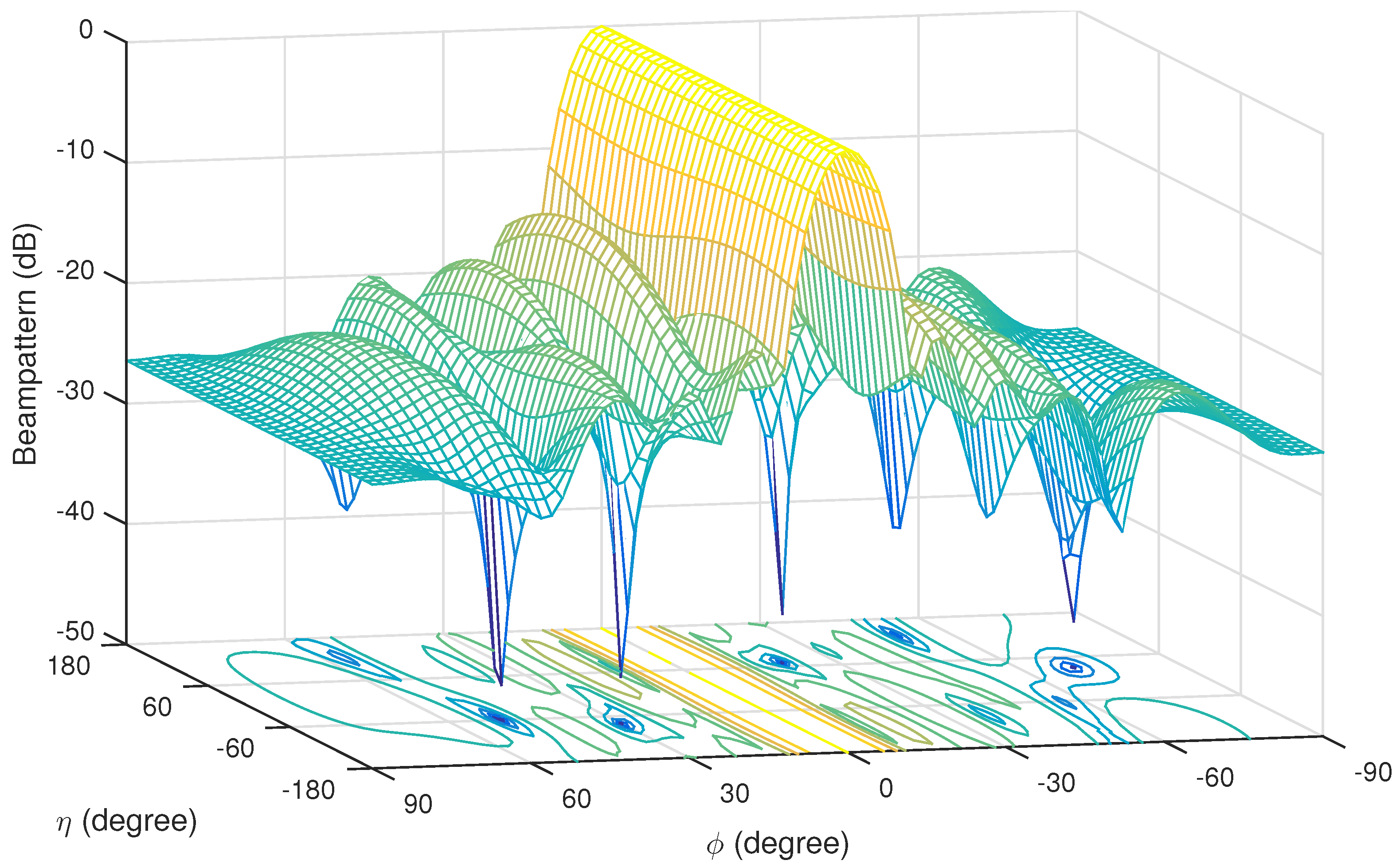
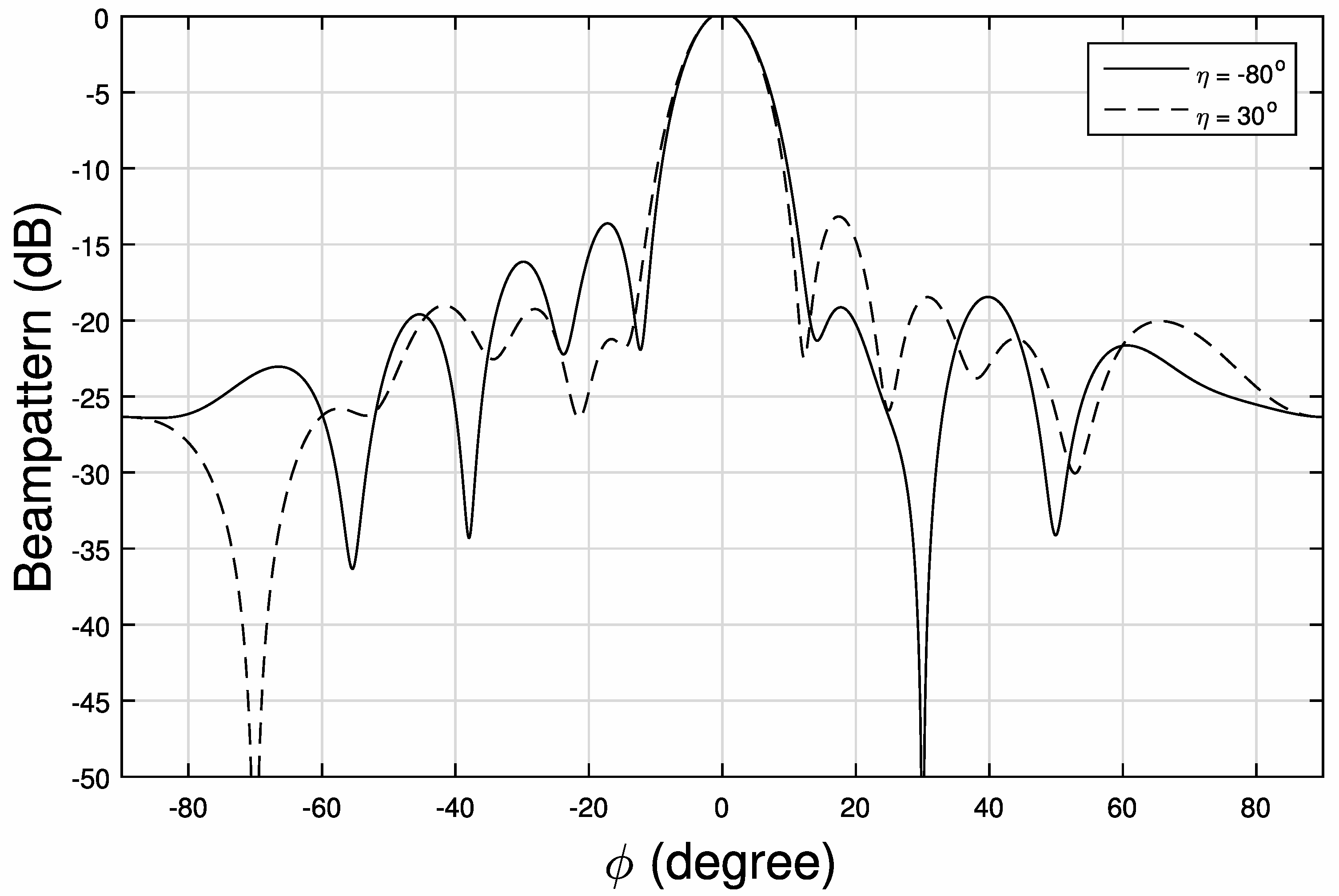
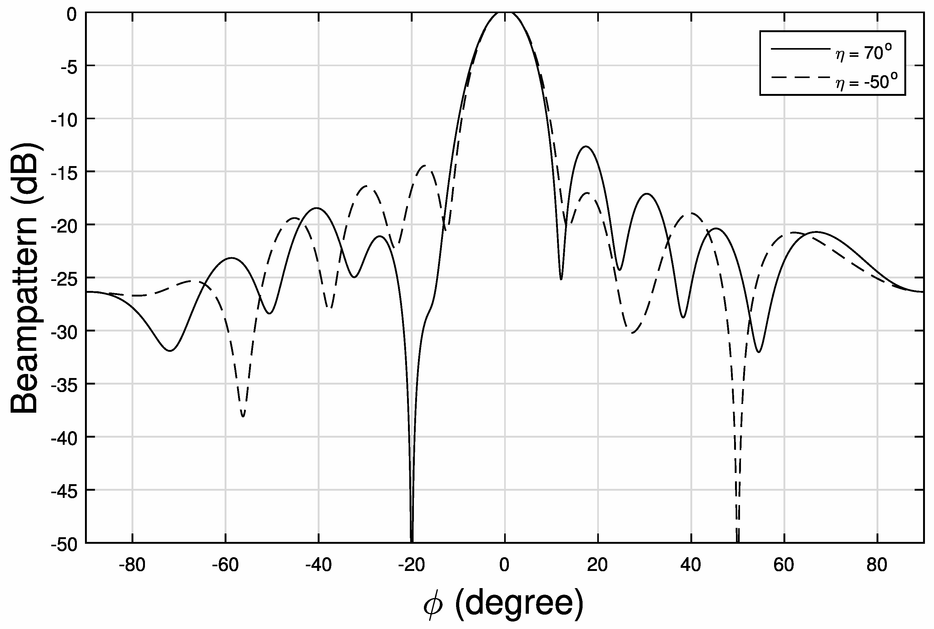
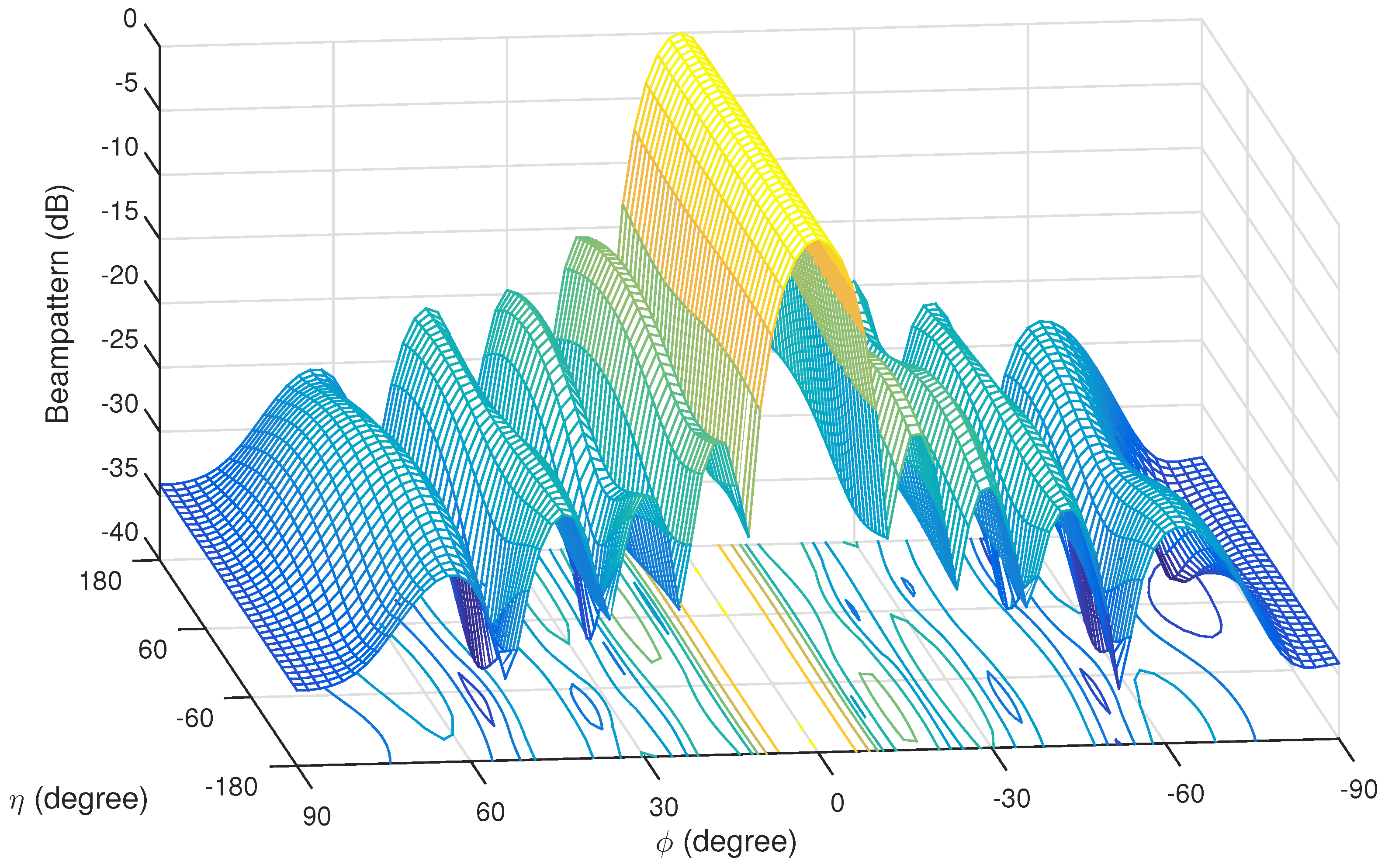
In this section, simulations results are provided in terms of the resultant beam pattern, output SINR, and robustness against steering vector mismatch. In the beam pattern part, both 2-D and 3-D beam patterns are presented for the proposed full Q-Capon beamformer to show the unity response to the desired signal and effective suppression to interferences. The beam pattern of the FQWCCB is also provided to show its tolerance around the desired DOA and polarization region. In the output SINR performance part, the full Q-Capon beamformer, FQWCCB, and the Q-Capon beamformer are compared in two scenarios: one without steering vector mismatch, and one with steering vector mismatch. A solid-line is also displayed as the optimal (ideal) beamforming result. The error constant $\epsilon$ for FQWCCB is set to $1.3$. In the robustness part, the beamformers are compared in terms of output SINR versus the snapshots number with 1° and 5° DOA and polarization mismatch errors, respectively.

5.1. Beam Pattern

We consider 10 pairs of cross-dipoles with half wavelength spacing. All signals are assumed to arrive from the same plane of $\theta =90$°, and all interferences have the same polarization parameter $\gamma =60$°. For the SOI, the two sub-signals are set to (90°, 1.5°, 90°, 45°) and (90°, 1.5°, 0°, 0°), with interferences coming from (90°, 30°, 60°, −80°), (90°, −70°, 60°, 30°), (90°, −20°, 60°, 70°), (90°, 50°, 60°, −50°), respectively. The background noise is zero-mean quaternion-valued Gaussian. The power of SOI and all interfering signals are set equal, and SNR (INR) is 20 dB.

Figure 2 shows the resultant 3-D beam pattern by the proposed full Q-Capon beamformer, where the interfering signals from ($\varphi ,\eta$) = (30°, −80°), (−70°, 30°), (−20°, 70°), and (50°, −50°) have all been effectively suppressed, while the gain of SOI from $\varphi =1.5$° stays almost constant.

Figure 2. Beam pattern obtained from the full Q-Capon beamformer with $\theta =90$° and $\gamma =60$°.

Figure 3 and Figure 4 show the 2-D beam patterns for $\eta =-80°,30°,70°,-50°$, respectively, where deep nulls have been formed at locations $\varphi =30°,-70°,-20°,50°$.

Figure 3. The resultant beam pattern for (1) $\theta =90°,\gamma =60°,\eta =-80°$; (2) $\theta =90°,\gamma =60°,\eta =30°$.

Figure 4. The resultant beam pattern for (1) $\theta =90°,\gamma =60°,\eta =70°$; (2) $\theta =90°,\gamma =60°,\eta =-50°$.

The 3-D beam pattern for the proposed FQWCCB is provided in Figure 5. We can still see that the interferences from ($\varphi ,\eta$) = (30°, −80°), (−70°, 30°), (−20°, 70°) and (50°, −50°) are suppressed, but the suppression is not as deep as in the case of the full Q-Capon beamformer; moreover, a large magnitude response are formed around the direction of the desired signal.

Figure 5. The resultant full quaternion worst-case constraint beamformer (FQWCCB) beam pattern with $\theta =90°$ and $\gamma =60°$.

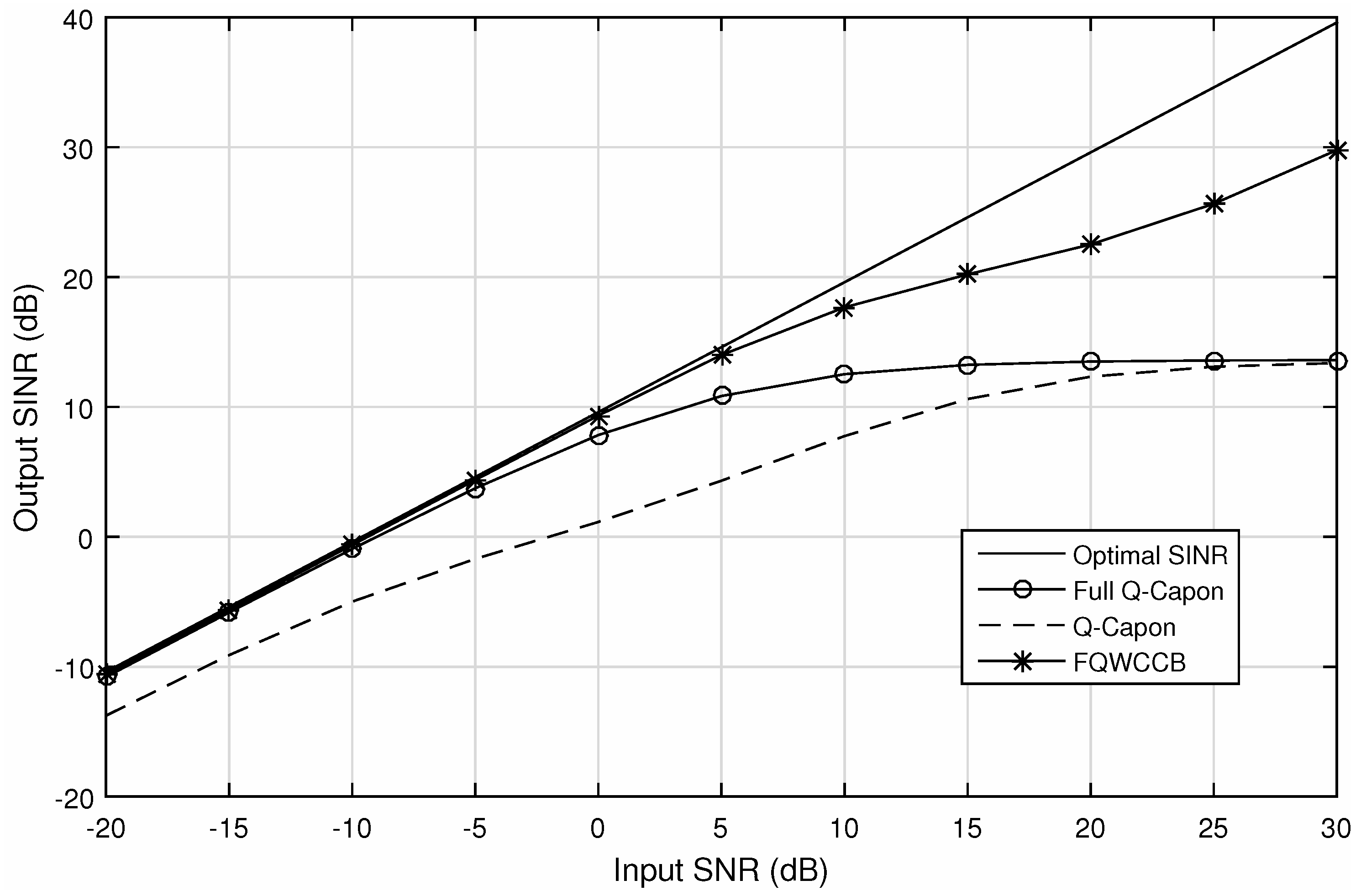
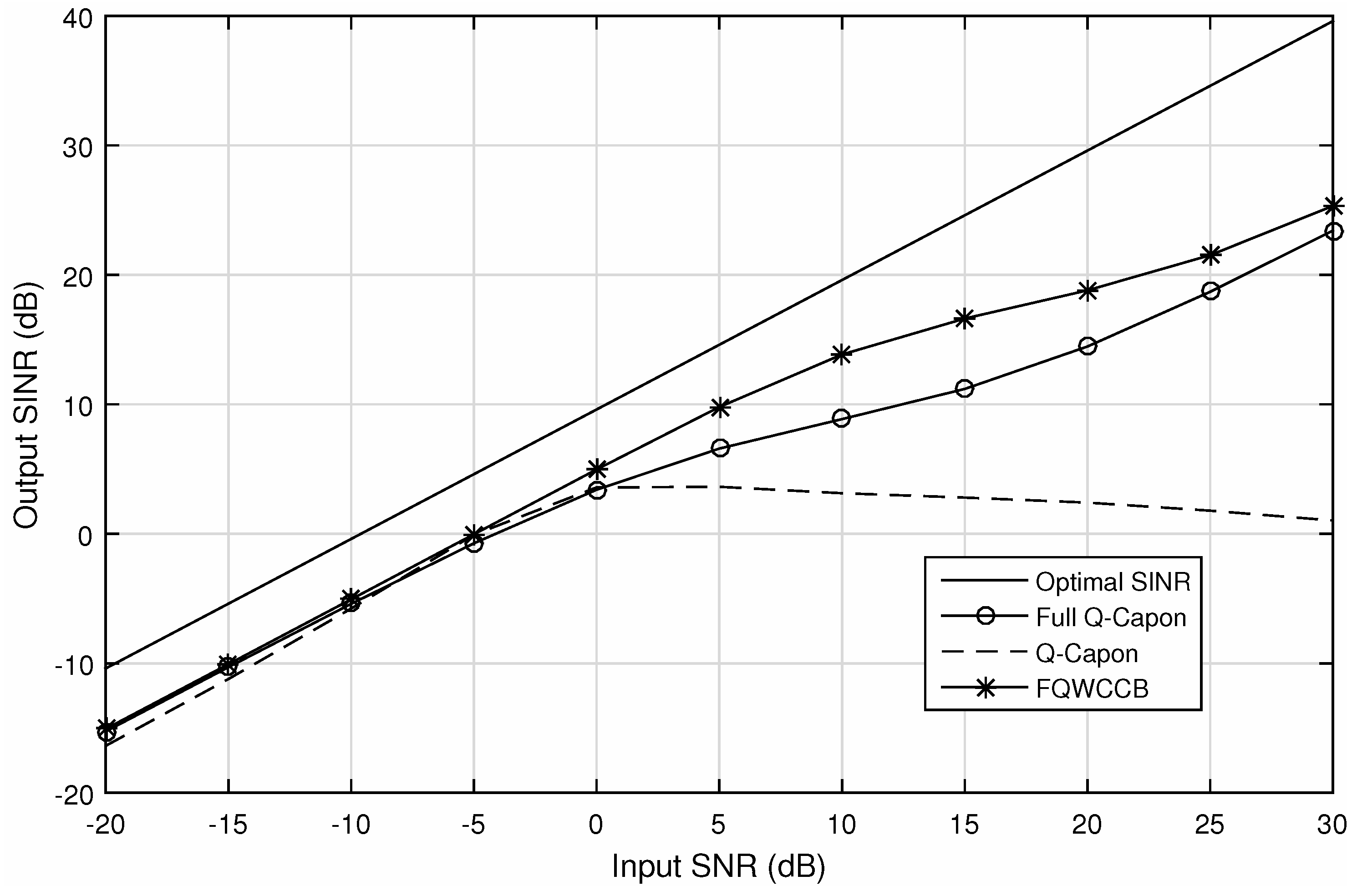
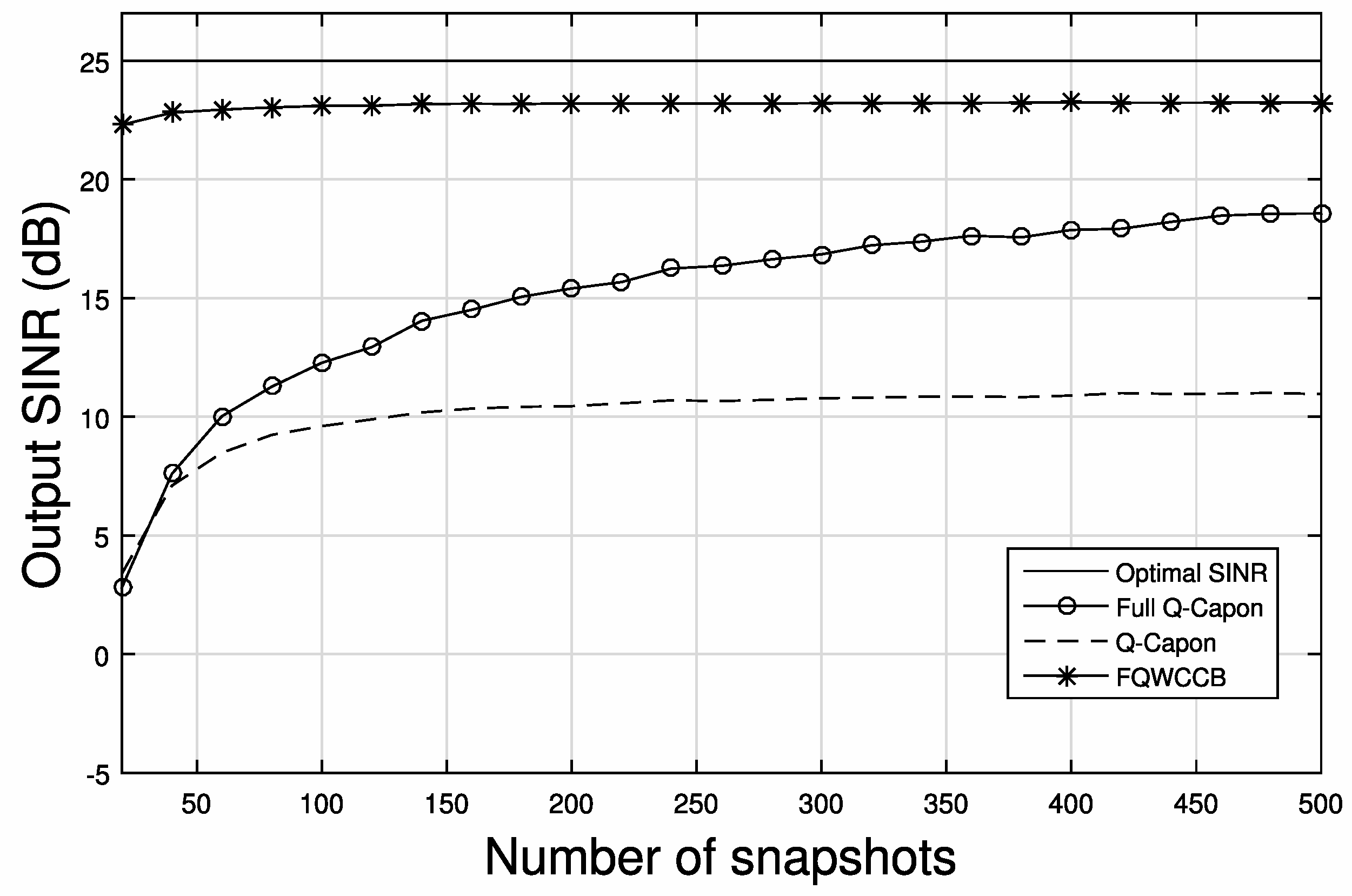
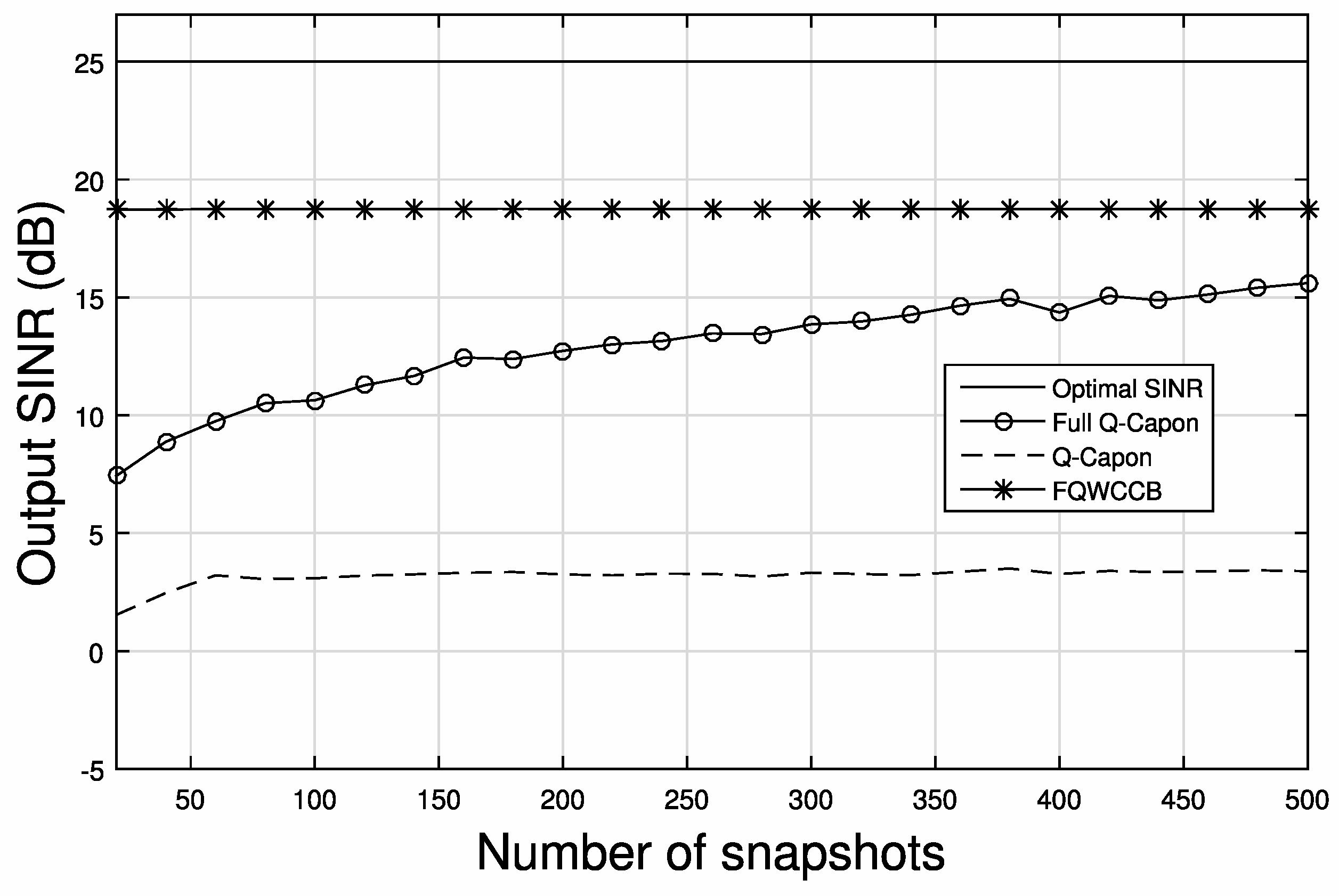
5.2. Output SINR Performance

In the following, the output SINR performance of the two Capon beamformers (full Q-Capon and Q-Capon) is studied with the DOA and polarization (90°, 1.5°, 90°, 45°) and (90°, 1.5°, 0°, 0°) for SOI and (90°, 30°, 60°, −80°), (90°, −70°, 60°, 30°), (90°, −20°, 60°, 70°), (90°, 50°, 60°, −50°) for interferences, respectively. Again, we have set SNR = INR = 20 dB. All results are obtained by averaging 1000 Monte-Carlo trials.

Firstly, we consider a scenario without steering vector mismatch. Figure 6 shows the output SINR performance versus SNR with 100 snapshots, where the solid-line is for the optimal beamformer (i.e., with infinite number of snapshots). Note that with only 100 snapshots, there will be non-negligible data model errors. It can be seen that for most of the input SNR range, the FQWCCB has the best output SINR performance versus the input SNR, while the full Q-Capon has a worse performance, but it still outperforms the Q-Capon beamformer. In the lower SNR range, FQWCCB and the full Q-Capon beamformer have a similar result, but the gap becomes greater from input SNR = 10 dB onwards. Additionally, in the lower range, the proposed full Q-Capon beamformer has a better performance than the Q-Capon beamformer; for very high input SNR values, these two beamformers have a very similar performance.

Figure 6. Output signal-to-interference-plus-noise ratio (SINR) versus input signal-to-noise ratio (SNR) for snapshots number 100, without steering vector mismatch.

Next, another set of simulations is performed in a similar setting, which is shown in Figure 7. The only difference is that there is 5° DOA and polarization mismatch for the SOI: the actual parameters of the two desired sub-signals are (95°, 6.5°, 95°, 50°) and (95°, 6.5°, 5°, 5°). For lower input SNR values (from −20 dB to 0 dB), the three beamformers have a similar output SINR, all worse than the example without steering vector mismatch. As the input SNR increases, difference among the three beamformers appears. From SNR = 0 dB onwards, the output SINR of FQWCCB and the full Q-Capon beamformer continue to increase, while the output SINR of the Q-Capon beamformer starts to drop slowly. Compared with the full Q-Capon beamformer, the FQWCCB has roughly achieved a 3 dB higher output SINR than the full Q-Capon beamformer, which means that the FQWCCB has a better performance than the full Q-Capon beamformer.

Figure 7. Output SINR versus input SNR for snapshots number 100, with 5° mismatch.

5.3. Performance with DOA and Polarization Mismatch

Next, we investigate their performance in the presence of both DOA and polarization errors with SNR = SIR = 15 dB. The output SINR with respect to the number of snapshots is shown in Figure 8 in the presence of 1° error for the SOI, where the actual DOA and polarization parameters are (91°, 2.5°, 91°, 46°) and (91°, 2.5°, 1°, 1°).

Figure 8. Output SINR versus snapshot number with SNR = SIR = 15 dB and 1° error.

We can see that the FQWCCB has the best performance in the presence of DOA and polarization mismatch, with output SINR above 20 dB for a varied number of snapshots. Both the full Q-Capon beamformer and the Q-Capon beamformer experience a loss of SINR (below 5 dB at the beginning and increasing with the snapshots number). However, the full Q-Capon beamformer has still achieved a much higher output SINR than the Q-Capon beamformer, and this gap increases with the increase of snapshots number. Figure 9 shows a similar trend in the presence of a 5° error. For the Q-Capon beamformer, the output SINR stays below 5 dB with little fluctuation, while the full Q-Capon beamformer and its worst-case constraint version can achieve a relatively high output SINR level of above 15 dB with 500 snapshots. Overall, we can see that the proposed full Q-Capon beamformer (both with worst-case constraint and without worst-case constraint) is more robust against array steering vector errors than the original Q-Capon beamformer.

Figure 9. Output SINR versus snapshot number with SNR = SIR = 15 dB and 5° error.

6. Conclusions

In this paper, a full quaternion model has been developed for adaptive beamforming based on crossed-dipole vector sensor arrays, with a new full quaternion Capon beamformer derived. Different from previous studies in quaternion-valued adaptive beamforming, we have considered a quaternion-valued desired signal, given the recent research development in quaternion-valued communications. The proposed beamformer has a better performance and a much lower computational complexity than a previously proposed Q-Capon beamformer, and is also shown to be more robust against array pointing errors. Furthermore, based on this full quaternion model, the robust beamforming problem has also been studied in the presence of steering vector errors, and a worst-case-based robust beamformer was developed. The effectiveness of the full Q-Capon beamformer and the robustness of the further developed worst-case-based beamformer was verified by computer simulations.

References

- Compton, R., Jr. On the performance of a polarization sensitive adaptive array. IEEE Trans. Antennas Propag. 1981, 29, 718–725. [Google Scholar] [CrossRef]
- Nehorai, A.; Ho, K.C.; Tan, B.T.G. Minimum-noise-variance beamformer with an electromagnetic vector sensor. IEEE Trans. Signal Process. 1999, 47, 601–618. [Google Scholar] [CrossRef]
- Godara, L.C. Application of antenna arrays to mobile communications. II. Beam-forming and direction-of-arrival considerations. Proc. IEEE 1997, 85, 1195–1245. [Google Scholar] [CrossRef]
- Xu, Y.G.; Liu, T.; Liu, Z.W. Output SINR of MV beamformer with one EM vector sensor of and magnetic noise power. In Proceedings of the International Conference on Signal Processing, Montreal, QC, Canada, 17–21 May 2004; pp. 419–422. [Google Scholar]
- Le Bihan, N.; Mars, J. Singular value decomposition of quaternion matrices: A new tool for vector-sensor signal processing. Signal Process. 2004, 84, 1177–1199. [Google Scholar] [CrossRef]
- Miron, S.; Le Bihan, N.; Mars, J.I. High resolution vector-sensor array processing using quaternions. In Proceedings of the IEEE Workshop on Statistical Signal Processing, Bordeaux, France, 17–20 July 2005; pp. 918–923. [Google Scholar]
- Miron, S.; Le Bihan, N.; Mars, J.I. Quaternion-MUSIC for vector-sensor array processing. IEEE Trans. Signal Process. 2006, 54, 1218–1229. [Google Scholar] [CrossRef]
- Gong, X.; Xu, Y.; Liu, Z. Quaternion ESPRIT for direction finding with a polarization sentive array. In Proceedings of the International Conference on Signal Processing, Beijing, China, 26–29 October 2008; pp. 378–381. [Google Scholar]
- Tao, J.W.; Chang, W.X. A novel combined beamformer based on hypercomplex processes. IEEE Trans. Aerosp. Electron. Syst. 2013, 49, 1276–1289. [Google Scholar] [CrossRef]
- Tao, J.W. Performance analysis for interference and noise canceller based on hypercomplex and spatio-temporal-polarisation processes. IET Radar Sonar Navig. 2013, 7, 277–286. [Google Scholar] [CrossRef]
- Zhang, X.R.; Liu, W.; Xu, Y.G.; Liu, Z.W. Quaternion-valued Robust Adaptive Beamformer for Electromagnetic Vector-sensor Arrays with Worst-case Constraint. Signal Process. 2014, 104, 274–283. [Google Scholar]
- Jiang, M.D.; Liu, W.; Li, Y. Adaptive Beamforming for Vector-Sensor Arrays Based on Reweighted Zero-Attracting Quaternion-Valued LMS Algorithm. IEEE Trans. Circuits Syst. II Express Br. 2016, 63, 274–278. [Google Scholar] [CrossRef]
- Gou, X.; Xu, Y.; Liu, Z.; Gong, X. Quaternion-capon beamformer using crossed-dipole arrays. In Proceedings of the IEEE International Symposium on Microwave, Antenna, Propagation, and EMC Technologies for Wireless Communications (MAPE), Beijing, China, 1–3 November 2011; pp. 34–37. [Google Scholar]
- Isaeva, O.M.; Sarytchev, V.A. Quaternion presentations polarization state. In Proceedings of the 2nd IEEE Topical Symposium of Combined Optical-Microwave Earth and Atmosphere Sensing, Atlanta, GA, USA, 3–6 April 1995; pp. 195–196. [Google Scholar]
- Wysocki, B.J.; Wysocki, T.A. On an Orthogonal Space-Time-Polarization Block Code. J. Commun. 2009, 4, 20–25. [Google Scholar]
- Liu, W. Channel equalization and beamforming for quaternion-valued wireless communication systems. J. Frankl. Inst. 2016. [Google Scholar] [CrossRef]
- Li, J.; Stoica, P. (Eds.) Robust Adaptive Beamforming; John Wiley & Sons: Hoboken, NJ, USA, 2005. [Google Scholar]
- Liu, W.; Weiss, S. Wideband Beamforming: Concepts and Techniques; John Wiley & Sons: Chichester, UK, 2010. [Google Scholar]
- Vorobyov, S.A.; Gershman, A.B.; Luo, Z.Q. Robust adaptive beamforming using worst-case performance optimization: A solution to the signal mismatch problem. IEEE Trans. Signal Process. 2003, 51, 313–324. [Google Scholar] [CrossRef]
- Yu, L.; Liu, W.; Langley, R.J. Novel robust beamformers for coherent interference suppression with DOA estimation errors. IET Microw. Antennas Propag. 2010, 4, 1310–1319. [Google Scholar] [CrossRef]
- Hamilton, W.R., II. On quaternions; or on a new system of imaginaries in algebra. Lond. Edinb. Dublin Philos. Mag. J. Sci. 1844, 25, 10–13. [Google Scholar]
- Huang, L.; So, W. On left eigenvalues of a quaternionic matrix. Linear Algebra Appl. 2001, 323, 105–116. [Google Scholar] [CrossRef]
- Zhang, F. Quaternions and matrices of quaternions. Linear Algebra Appl. 1997, 251, 21–57. [Google Scholar] [CrossRef]
- Jiang, M.D.; Li, Y.; Liu, W. Properties of a General Quaternion-Valued Gradient Operator and Its Application to Signal Processing. Front. Inf. Technol. Electron. Eng. 2016, 17, 83–95. [Google Scholar]
- Capon, J. High-resolution Frequency-wavenumber Spectrum Analysis. Proc. IEEE 1969, 57, 1408–1418. [Google Scholar] [CrossRef]
- Frost, O.L., III. An algorithm for linearly constrained adaptive array processing. Proc. IEEE 1972, 60, 926–935. [Google Scholar] [CrossRef]
- Wang, M.; Ma, W. A structure-preserving algorithm for the quaternion Cholesky decomposition. Appl. Math. Comput. 2013, 223, 354–361. [Google Scholar] [CrossRef]
© 2017 by the authors. Licensee MDPI, Basel, Switzerland. This article is an open access article distributed under the terms and conditions of the Creative Commons Attribution (CC BY) license (http://creativecommons.org/licenses/by/4.0/).