Cooperative Path-Planning for Multi-Vehicle Systems

Abstract

In this paper, we propose a collision avoidance algorithm for multi-vehicle systems, which is a common problem in many areas, including navigation and robotics. In dynamic environments, vehicles may become involved in potential collisions with each other, particularly when the vehicle density is high and the direction of travel is unrestricted. Cooperatively planning vehicle movement can effectively reduce and fairly distribute the detour inconvenience before subsequently returning vehicles to their intended paths. We present a novel method of cooperative path planning for multi-vehicle systems based on reinforcement learning to address this problem as a decision process. A dynamic system is described as a multi-dimensional space formed by vectors as states to represent all participating vehicles’ position and orientation, whilst considering the kinematic constraints of the vehicles. Actions are defined for the system to transit from one state to another. In order to select appropriate actions whilst satisfying the constraints of path smoothness, constant speed and complying with a minimum distance between vehicles, an approximate value function is iteratively developed to indicate the desirability of every state-action pair from the continuous state space and action space. The proposed scheme comprises two phases. The convergence of the value function takes place in the former learning phase, and it is then used as a path planning guideline in the subsequent action phase. This paper summarizes the concept and methodologies used to implement this online cooperative collision avoidance algorithm and presents results and analysis regarding how this cooperative scheme improves upon two baseline schemes where vehicles make movement decisions independently.

1. Introduction

Many multi-vehicle systems exist. In this paper, we choose to focus on shipping. A common challenge facing shipping is potential collisions, particularly in busy regions, such as the English Channel. Shipping-related accidents can result in significant environmental damage. Furthermore, shipping is a significant contributor to greenhouse gas emissions, particularly with respect to diesel fuel exhaust gases, so avoiding long detours around potential hazards is desirable. Nevertheless, shipping presents a particularly challenging problem as rapid changes in speed are undesirable or impossible to achieve, whilst there are an infinite number of potential detour paths from which to choose.

The aim of this research is to examine how a number of vehicles can orchestrate their movements so as to deviate little from their intended path whilst avoiding collisions between them, as well as obstacles. The assumption is that the degree of movement “inconvenience” (i.e., the magnitude of the detour) should be apportioned fairly among the vehicles concerned. Although stopping or changing speed are strategies to avoid collisions requiring little or no deviation from the intended path, they can consume significant energy. Conversely, we assume vehicles continue to travel at a constant speed. This means the path-planning solution should be optimized to some extent to allow vehicles to detour efficiently without the need to adjust speed. The “inconvenience” is a measure of how much energy is consumed in steering the ships from their intended path. Ideally, the goal is to minimize this.

Collision avoidance for multiple vehicles is an important research topic. Most of the early research explored the problem of two-dimensional path-planning in the context of a group of robotic vehicles travelling to avoid stationary obstacles [1,2]. More recently, researchers have addressed the importance of collision avoidance amongst vehicles. In some approaches [3,4], for each vehicle, other vehicles are regarded as mobile obstacles. A given vehicle predicts where the others might be in the future by extrapolating their observed velocities and avoids collisions accordingly. In [4], a collision-free navigation method for a group of unmanned autonomous vehicles is introduced. The position and orientation information of the individuals is transformed into variables to produce navigation data for each of them. However, this solitary method does not impose constraints on the vehicle speed or turn radius. As such, what may be a safe manoeuvre with respect to the current time step can lead to collisions in the future. Indeed, vehicles may be required to change course instantaneously, which is not possible in many practical instances due to the kinematic constraints of the vehicles involved. In other research, parametric curves are adopted to model the path to guarantee that all mobile vehicles in the system can perform smooth detours and eventually arrive at their intended goal [5,9,10,11]. However, to track these paths, vehicles have to constantly change their speed and orientation, and the magnitude of this change can be quite large, which is also not realistic. As a result, we make the same assumption as in [6,12], that is vehicles travel at a constant speed and gradually change orientation by taking circular arcs. This allows the proposed algorithm to be straightforward to execute in real time, even for relatively large-scale path-planning scenarios.

In [7,8] each vehicle calculates its own near optimal path and plans its motion in isolation by following a collection of local rules. A localized path-planning scheme for soccer robots is presented in [7]; the limited turning radius and speed constraints of the robots are considered. However, in many cases, localized path-planning schemes cannot cope with arbitrary traffic due to the kinematic randomness of the individuals involved. In other research [9,10,11], heuristic methods, such as genetic algorithms, have been employed to find solutions to this problem by taking into account every vehicle in the system. For example, research in [9,10] presents a near-optimal collision avoidance scheme between multiple robots, which enables them to avoid potential collisions cooperatively without introducing any new ones. However, if a vehicle experiences multiple potential collision events, it is difficult to reconfigure its trajectory, because the scheme requires considerable computational effort. As a result, it is not feasible for “on the fly” path-planning.

Reinforcement learning (RL) is a powerful technique for solving problems that are challenging, because they lack mathematical models to address how the information should be processed [13]. Assuming a system is to transit to its goal state, there are typically a great many strategies it could employ. In order to approximately determine the best policy, RL can be employed. Most RL algorithms focus on approximating the state or state-action value function. For value function-based algorithms, the goal is to learn a mapping from states or state-action pairs to real numbers that can approximately represent the desirability of each certain state or state-action combination. The state value function determines how good the current state is, but it is not sufficient for acting upon it. In order to find the best action to take from the current state, we need a model to calculate possible next states. Experience is gained by interacting with the environment. At each interaction step, the learner observes the current state s, chooses an action a and observes the resulting next state s' and the reward received r, essentially sampling the transition model and the reward function of the process. Thus, experience can be expressed in the form of (s, a, r, s') samples.

Our approach is to devise a cooperative collision-avoidance path-planning scheme that can produce sequences of manoeuvring decisions in real time using RL. The goal of the scheme is to determine an adaptive control law to generate a good path solution for all of the cooperating vehicles involved, rather than to assign them a fixed set of rules to follow. This article is an expanded version of a paper entitled “Cooperative collision avoidance for multi-vehicle systems using reinforcement learning” presented at the 18th International Conference on Methods and Models in Automation and Robotics (MMAR), Miedzyzdroje, August 26–29, 2013 [14]. In addition to providing a more in-depth explanation of the proposed scheme, we now compare it with two other approaches to show the benefit of cooperative planning in terms of success rate, detour inconvenience and fairness. We also investigate how the number of participating vehicles affects the performance.

2. Related Work

Path-planning has been a topic of research in many areas, including robotics and navigation. Most of the early research explored the problems of two-dimensional or three-dimensional path-planning in the context of a point-like vehicle travelling to avoid circular danger regions [1]. Generally, path-planning problems can be divided into two categories. The first category considers problems of how to plan a path when the locations of all of the “dangers” are known [15]. The solution to this problem gives the vehicle a (near) optimal path to follow even before it leaves the starting point. In the second category, the locations of the dangers are unknown in advance. They can only be acquired if they are within the vehicle’s sensing range [2,3]. The vehicle changes its path when it senses danger areas. This second problem category is sometimes referred to as dynamic path-planning.

Since the late 1990s, more research has been conducted on path-planning algorithms for mobile robots and unmanned aerial vehicles (UAVs), such as the work in [6,11,16]. These path-planning schemes can be categorized with regard to the number of objective robots or UAVs being considered.

One class of problem is where the robot or UAV is moving in a constrained environment. For example, a growing role in the field of unmanned aerial vehicles (UAVs) is the use of unmanned vehicles to conduct electronic countermeasures [17]. When performing electronic countermeasures, a set of checkpoints is generated for the UAV, which satisfy particular environmental constraints. The UAV must follow these checkpoints with specific states, which depend on the requirement of the task being carried out. Many papers, such as [18,19], discuss how to determine feasible paths for a UAV to avoid radar networks that contain several radars that may have different coverage characteristics.

A geometry-based path-planning algorithm was introduced in [17]. The algorithm can find the shortest path from a starting point to a goal point, whilst meeting the heading constraints of the UAV. However, the planned path cannot guarantee guiding the UAV to completely avoid radar installations; furthermore, the magnitude of changes in speed can be as big as 80%, which is not generally realistic. In the work described in [16], an approach based on a genetic algorithm is proposed, which is able to find suboptimal solutions. However, it does not take into account any kinematic constraints of the vehicle, so it imposes extremely demanding requirements on the unmanned vehicles.

Another class of problems considers where multiple robots or UAVs perform a group task [20]. In the last decade, the idea of using UAVs for surveillance, patrol and rescue missions has emerged. A group of UAVs are typically required in missions like these to cover the search region. These vehicles should cooperate to ensure the effectiveness of the mission and to prevent potential collisions between vehicles. However, designing a cooperative path-planning algorithm for these tasks is much more complex than for a single vehicle. The difficulty arises due to several reasons. Firstly, limited sensor range constrains each vehicle’s response time, which makes it difficult to steer efficiently. Next, limited communication range prevents vehicles from working cooperatively when they are too far apart. In addition, the acceptable processing time is limited. Path-planning is required to solve real-time optimization problems, but due to limited computational performance, optimal solution(s) can be difficult to determine in a short time. Finally, obstacles or hostile entities present in the region of operation may be mobile, which typically requires a motion prediction capability to anticipate their movements. An effective multi-agent coordination scheme must handle these issues. It should be flexible and adaptive, allowing multi-agent teams to perform tasks efficiently.

In [21], the authors present a cognitive-based approach for solving path-planning problems using multiple robot motion management, which features excellent reduction in the computation cost. However, the solutions are often not smooth paths. The abrupt changes in speed and direction can cost much energy, which is typically unacceptable. Furthermore, short detour paths are not guaranteed.

In some schemes, vehicles are required to maintain certain formations whilst avoiding collisions. Formation control is a particular method deployed among robotic vehicles with limited sensing and communication range [22,23]. A typical application of multi-robot systems is object transportation. In this task, several robots move in a coordinated manner to move an object from a given starting location to a goal location and orientation, with associated performance requirements. The work introduced in [24] shows how a group of robots can be made to achieve formations using only local sensing and limited communication. Based on graph theory, the authors of [25] define a structured “error of formation” and propose a local control strategy for individual robots, which can ensure multiple robots converge to a unique formation. Among all of the approaches to formation control introduced in the literature, the method proposed in [26,27] has been adopted by most researchers. In this scheme, each robot takes another robot in its vicinity as a reference node to determine its motion. However, the complexity of the path-planning problem increases enormously even when only a single additional robotic vehicle is introduced. The required computational effort to achieve a real-time solution for a large vehicular network would be unfeasible.

Another popular means of classifying path-planning is in regard to local planning or global planning [28,29,30]. In local path-planning, a vehicle or robot navigates through the route step-by-step and determines its next position towards the goal as it proceeds (i.e., online planning), satisfying one or more predefined constraints in relation to the path, time or energy optimality [31,32]. In global planning, however, every vehicle plans the entire path before moving towards the goal. This type of planning is sometimes referred to as offline planning [33].

Research in [9,10] presents an offline cooperative collision avoidance scheme between multiple robots based on Bézier curves, which is the most similar state-of-the-art approach to ours. However, it is only capable of planning for a limited number of robots to determine their optimized paths in terms of the shortest overall distance travelled. The algorithm manages to avoid all potential collisions without introducing any new ones. Nevertheless, it requires considerable computational effort. Conversely, our method, described in Section 4, may create other potential collision domains whilst navigating around the current one; however, it re-invokes itself to solve these new potential collisions until none remain. In addition, the research in [9,10] is designed for robots performing group tasks, which means it cannot guarantee that these robots will not have collisions with non-cooperative mobile objects. Instead, our method considers potential problem(s) in chronological order; thus, potential collisions resulting from intruders (i.e., non-cooperative vehicles) or newcomers can be addressed.

Recently, reinforcement learning (RL) [34], sometimes referred to as approximate dynamic programming (ADP) [35,36], has been investigated for use in differential games, such as air combat between two UAVs. In [37,38,39], various RL methods are used to obtain fast solutions as required in a tactically changing environment. In [37], where the mission management issues of UAVs in adversarial environments are investigated, a heuristic is developed to decouple the control commands and to reduce computational expense. The work presented in [39] introduces hierarchically accelerated dynamic programming (HADP), which is an approximation method used to reduce computation time for dynamic programming; however, it only works effectively on finite state spaces and is difficult to adapt to infinite state spaces. The work presented in [38] deals with optimizing the evasive motion for one UAV against a chaser whose manoeuvring tactics are based on the technique proposed in [40]. It successfully produces realistic manoeuvring in response to adversaries. The state space is sampled for computational tractability, and the reward function is approximated. Due to the high dimensionality and continuity of the state space, a least squares estimate and a rollout extraction method are used to search for a near-optimal solution.

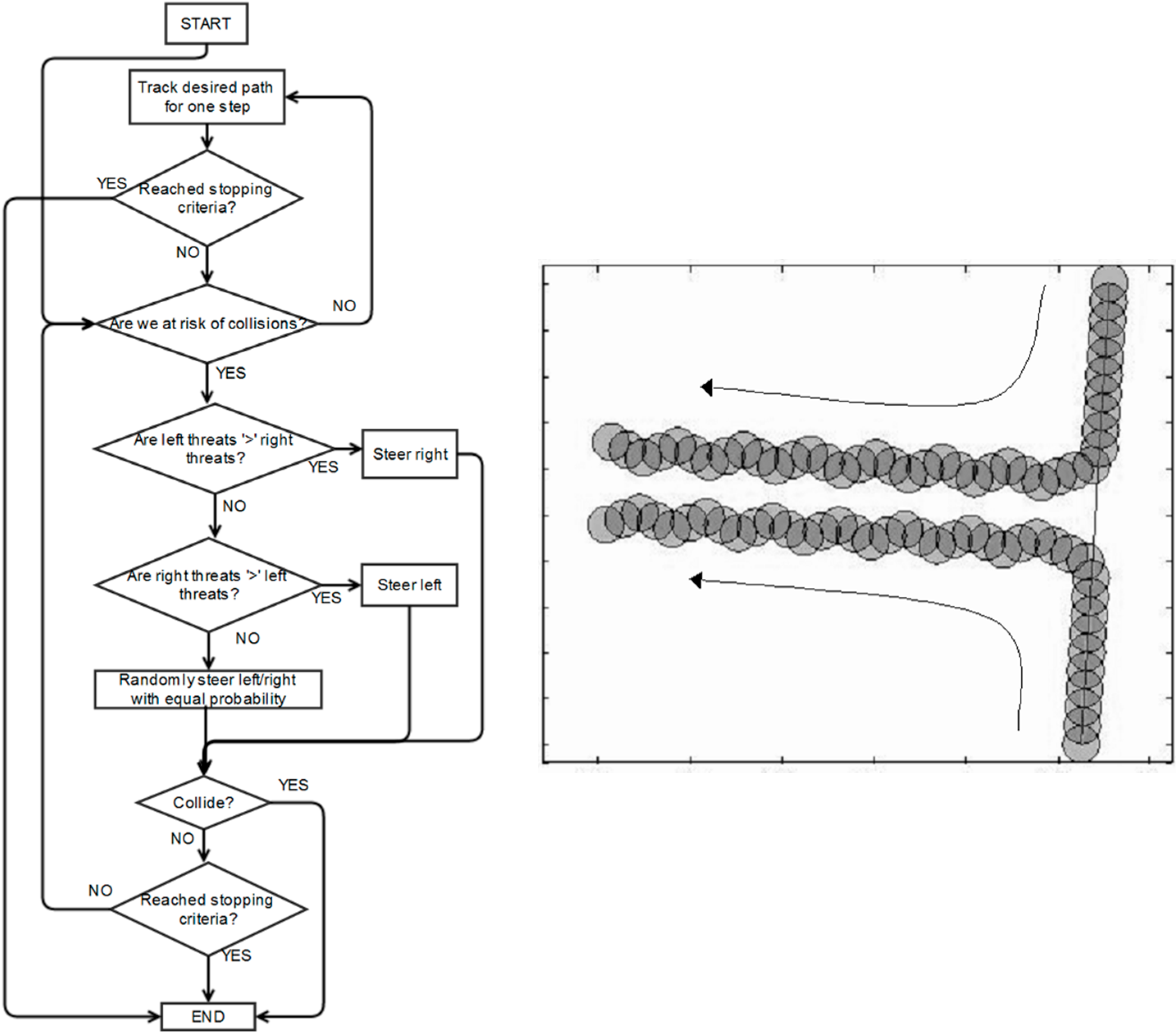
3. Problem Description

This section introduces the proposed cooperative path-planning scheme from a functional perspective with the following assumptions and requirements:

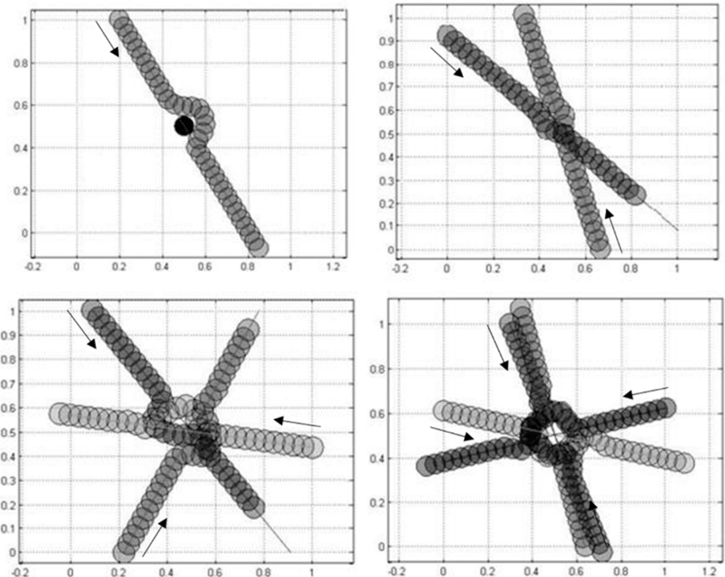
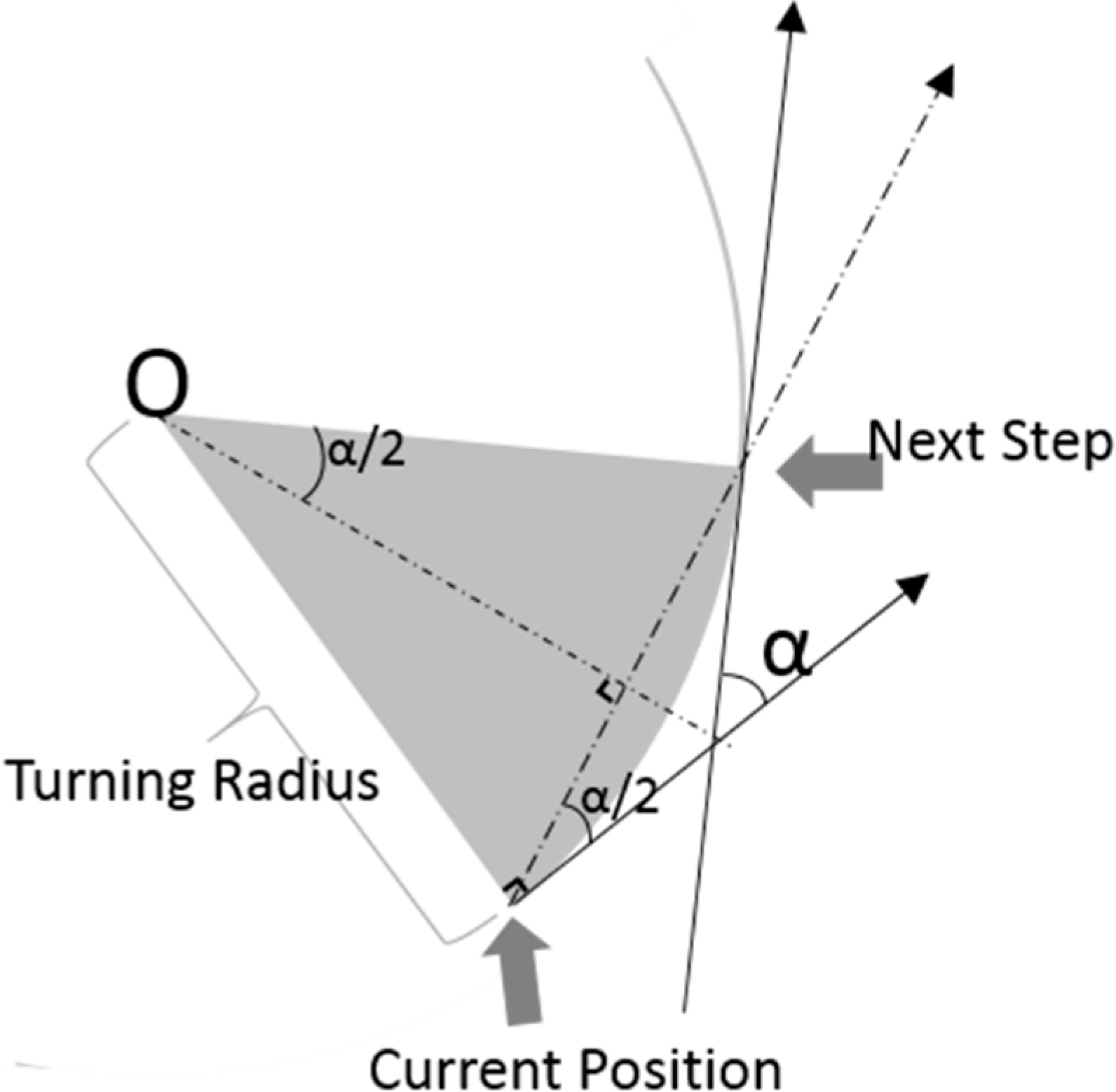
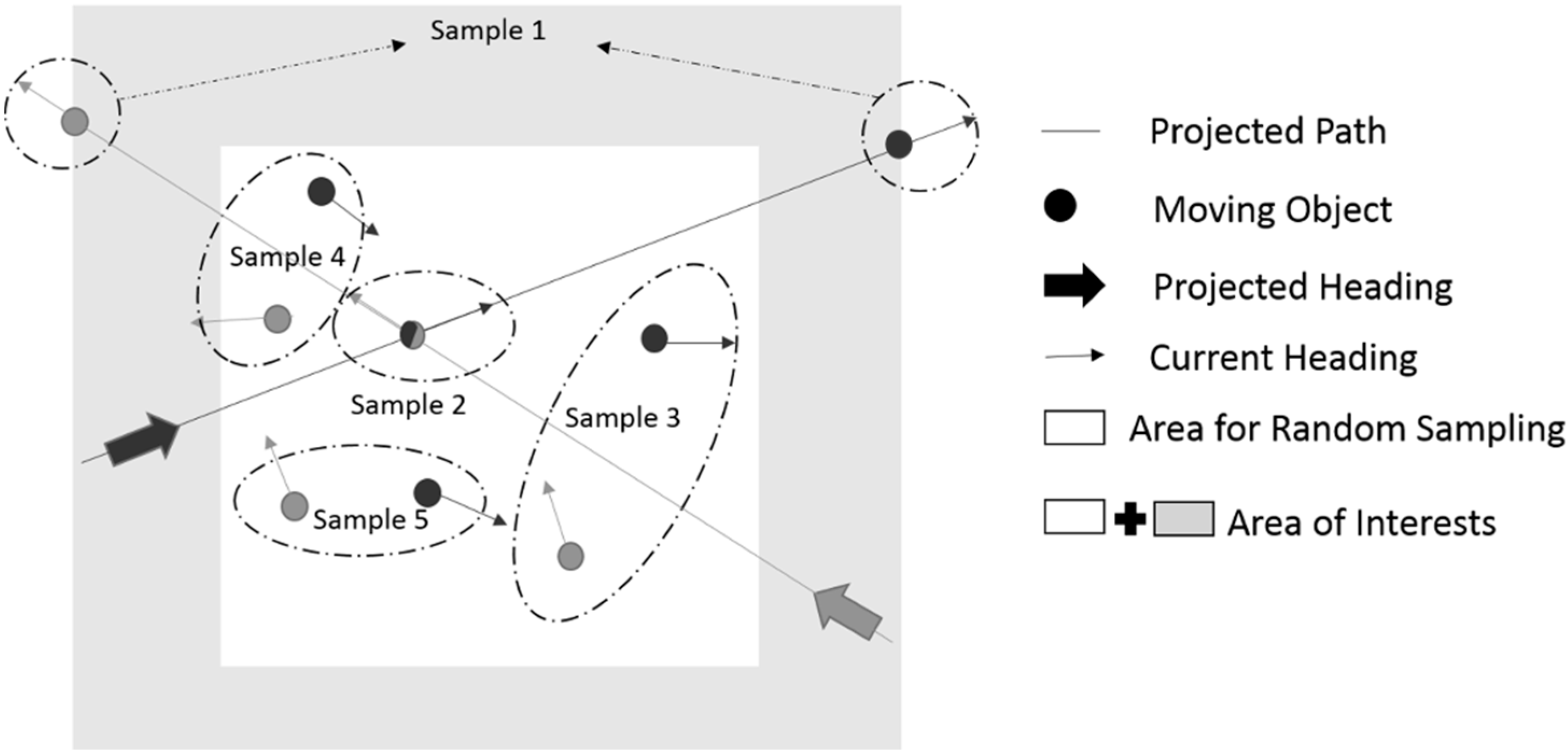
Though vehicles come in different shapes and sizes, vehicles modelled in this scheme are circular and of the same size. Further details are given in Section 7. They are assumed to travel at a constant speed and can gradually change direction by following circular arc tracks. The area of interest is a square surface where each vehicle starts from some point along one edge and is initially projected to travel in a straight line to another point along the opposite edge. Within the area of interest, they can communicate with each other in order to share their intended detour motions.

The scheme should be able to provide collision-free smooth paths for all vehicles whilst ensuring that they detour efficiently, cooperatively and fairly, which imposes a series of constraints on the optimization problem as listed. If the position of each of n vehicles is presented in a 2D Cartesian coordinate system and x, y represent the coordinates at time t, each of them has an initial position given by:

$$x_i(0)=x_{i,start},y_i(0)=y_{i,start}$$

(1)

Then, a vehicle travels at constant speed v_i, such that:

$$\forall t>0:\sqrt{{({\dot{x}}_i(t))}^2+{({\dot{y}}_i(t))}^2}=v_i$$

(2)

It should keep beyond a certain distance d_min from others, thus:

$$\forall t>0,i\ne j:\sqrt{{(x_i(t)-x_j(t))}^2+{(y_i(t)-y_j(t))}^2}\ge d_{\text{min},ij}$$

(3)

It should return to its desired path L_i after avoiding collisions at some point in time t_{finish, i}:

$$\exists t_{finish,i}:(x_i(t_{finish,i}),y_i(t_{finish,i}))\in L_i$$

(4)

As vehicles travel at constant speed, the goal is to reduce the sum of the time all vehicles spend performing evasive manoeuvres, i.e.,

$$\text{cost}={\displaystyle \sum }_{i=1}^n{t}_{finish,i}$$

(5)

Path planning in this research is regarded as a decision process. At each time step, the system determines appropriate steering motions for all vehicles. States in this system represent the position and orientation of all vehicles; thus, the system is multi-dimensional, and state transitions in this system constitute the planning problem. States featuring vehicles travelling along their desired path without potential collisions are the goal states. The system upon reaching a goal state terminates the transition process. Actions, i.e., the rules of transition between states, are represented by multi-dimensional vectors that represent the angular velocity of all vehicles. The action set is a multi-dimensional bounded continuous space where each vehicle’s minimum turning radius constraint is considered. Transition decisions are made by maximizing the reward of getting to a goal state from the current state, whilst the optimum transition policy is unknown. As the transition process is step-wise, it would at first appear to be a Markov decision process.

In this context, a Markov decision process (MDP) is a six-tuple (S, A, P, R, γ, D), where S is the state space of the system, A is the action space of the system, P is a Markovian transition model, P(s'│s, a) denotes the probability of getting to state s' after taking action a at state s and R is a reward function. R(s, a) is thus the reward for taking action a in state s, γ ϵ (0, 1] is the discount factor for delayed rewards and D is the initial state distribution. A common way to solve the problem of MDPs is estimating value functions, that is functions of states or state action pairs that reflect how “good” it is for an agent to be in a given state or to perform an action from a given state [41]. In the context of functions of states, a policy π is a mapping from each state s ϵ S and action a ϵ A(s), to the probability of taking action a when in state s. Therefore, the value V_π(s) of a state s under policy π is the expected total return when the system starts at time t in state s and follows π thereafter. For MDPs, it is formally defined as follows:

$$V_{\pi }(s)=E_{\pi }\{R_t|s_t=s\}=E_{\pi }\{{\displaystyle \sum _{k=0}^{\infty }{\text{γ}}^k}{r}_{t+k+1}|s_t=s\}$$

(6)

However, another way to describe the decision process is to use the value Q_π(s, a) of a state-action pair (s, a) under policy π. Q_π(s, a) is defined as the expected total discounted reward when the system transits from state s by taking action a:

$${\text{Q}}_{\pi }(s,a)=E_{\pi }\{R_t|s_t=s,a_t=a\}=E_{\pi }\{{\displaystyle \sum }_{k=0}^{\infty }{\text{γ}}^k{r}_{t+k+1}|s_t=s,a_t=a\}$$

(7)

The goal of the decision process is to find an optimal policy π* for selecting actions, which maximizes the total discounted reward for states drawn from D:

$$\pi *=\text{arg}\underset{\pi }{\text{max}} E_{s~D}\{V_{\pi }(s)\}=\text{arg}\underset{\pi }{\text{max}} E_{s~D}\{{\text{Q}}_{\pi }(s,a)\}$$

(8)

There is at least one optimal policy for every MDP. If an optimal value function V_π*(s) or Q_π*(s, a) is known, the corresponding optimal policy π* can be obtained only if the MDP model is known to support one-step lookaheads.

However, the state space and action space in this research are multi-dimensional and continuous, so reinforcement learning (RL) is therefore adopted to solve this MDP problem and efficiently handle the dimensionality scalability issue and permit working with a continuous space. In RL, a learner interacts with a decision process in a value function mechanism, as previously described, using Watkins’ Q-learning method [41] or Sutton’s temporal difference (TD) method [42]. The goal is to gradually learn a good policy using experience gained through interaction with the process.

The proposed scheme has two phases that can be described as “learning” and “action”. In the learning phase, inspired by the TD method, the system iteratively learns the scoring scheme for each state, which is basically affected by the reward of transition to its closest goal state. An approximate value function of the state-space is obtained at the end of the learning phase that is able to score any particular state in the system. In the action phase, for each time step, the system is able to move the vehicles to a viable next state with a relatively high score that corresponds to a position with a low risk of potential collisions and a good prospect of returning to the intended path. This algorithm is tested in MATLAB using a variety of scenarios to confirm its viability.

4. Path-Planning Based on Reinforcement Learning

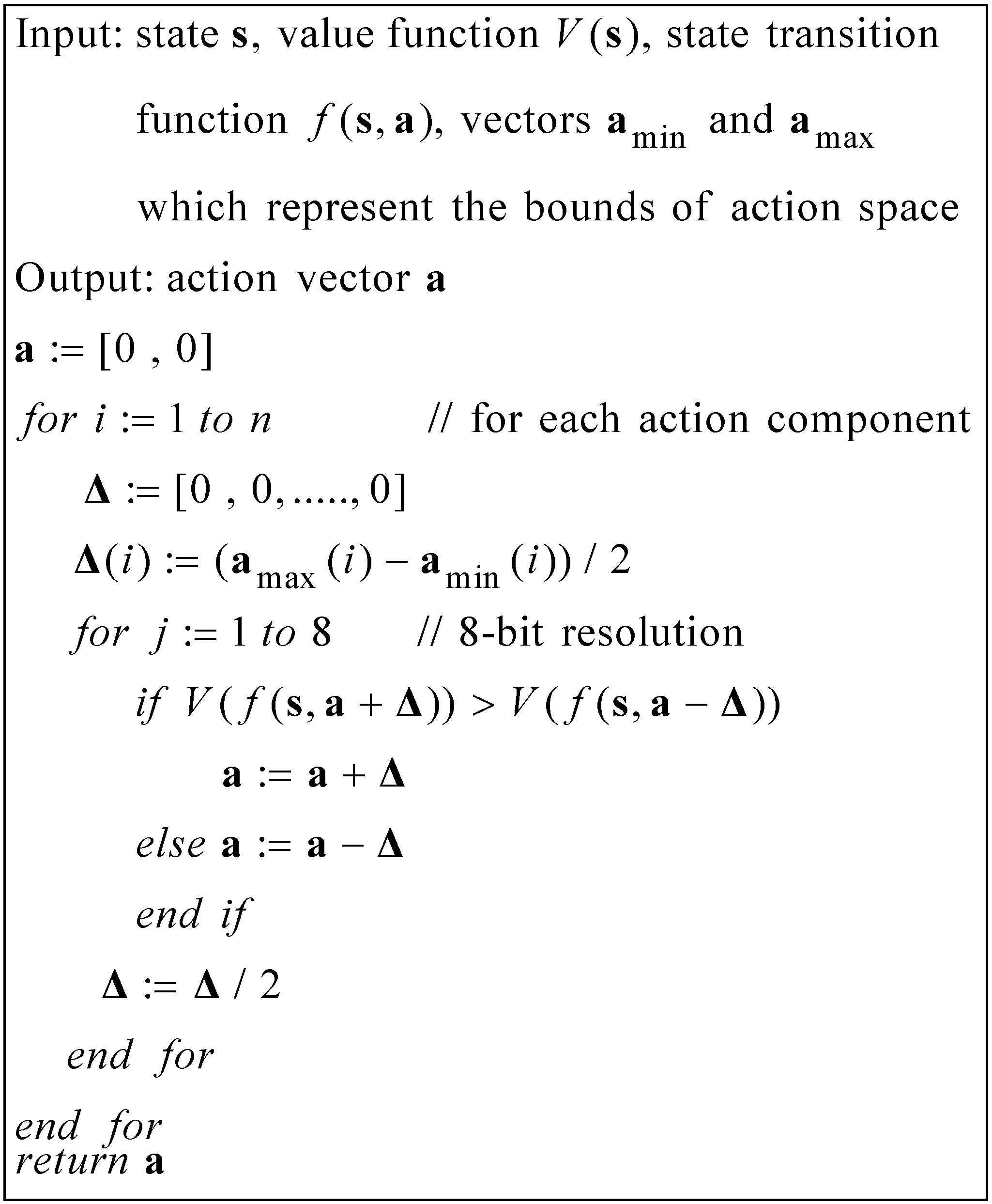
If there are many viable actions to take from the current state, evaluating all of them explicitly is not feasible. Therefore, an approximate search algorithm is required. In this section, concepts associated with RL are described and then specified in accordance with the state value function approach.

A state in the system takes the coordinates of multiple vehicles, describing the position and orientation of them at the same time. The state-space is bounded and holds all possible combinations of the position and orientation of these vehicles. For example, in simulations where only pairs of vehicles are considered, a state $s\in {\text{R}}^6$ is represented as:

$$s=[x_1^{pos},y_1^{pos},{\text{θ}}_1,x_2^{pos},y_2^{pos},{\text{θ}}_2],0\le {\text{θ}}_1,{\text{θ}}_2<2\text{π}$$

(9)

where θ represents the orientation, which is a number in the range zero to 2π. x^pos and y^pos are Cartesian coordinates.

Actions are defined as rule(s) that indicate how the system can make a transition to its next state. In the simulations, vehicles have a fixed speed and a changeable, but limited, turn radius. In two-vehicle simulations, the vehicles’ speeds are denoted as v₁ and v₂. The minimum turn radii are denoted as $r_1^{\text{min}}$ and $r_2^{\text{min}}$ . An action, denoted as a, is a combination of both vehicles’ possible motions. The motion pair $a\in {\text{R}}^2$ is described in terms of orientation variation, as follows:

$$a=[a_1,a_2],-\frac{v_i}{r_i^{\text{min}}}\le a_i\le \frac{v_i}{r_i^{\text{min}}}\hspace{0.17em}\text{where} i = 1,2$$

(10)

Actions that lead the vehicles out of the state-space are not permitted.

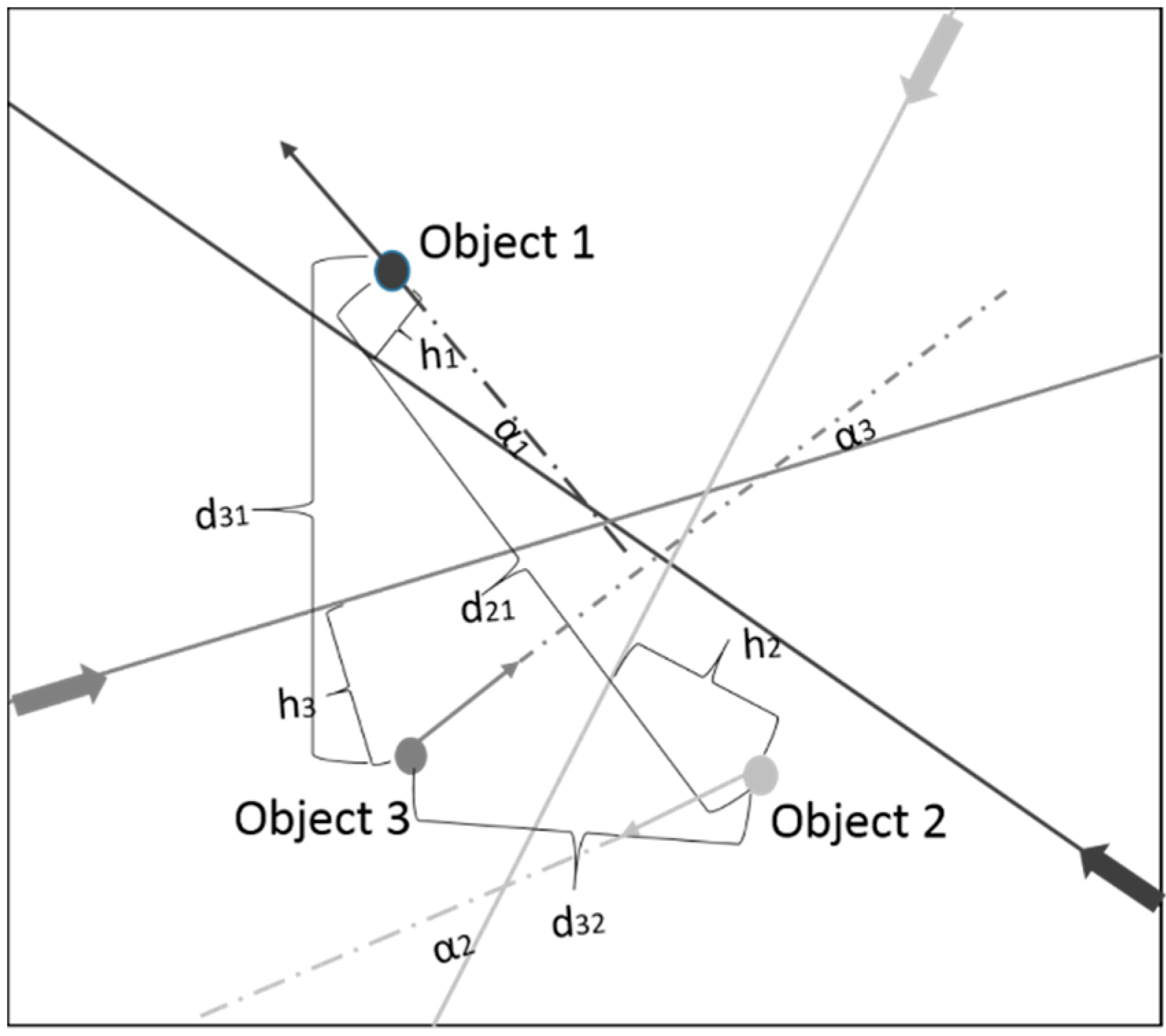
A reward is a fixed value attached to a state. In the simulations, as vehicles are permitted to take detours and then return to their projected paths, the goal states are states where both vehicles are on the projected paths with appropriate orientations, and they have a major positive reward. Forbidden states are states that suggest that the vehicles collide with each other or with obstacles, so that they have a major negative reward. d_min is the minimum distance allowed between two vehicles, and d(s) is the current distance between vehicles. Forbidden states are states that meet the condition:

$$d(s)=\sqrt{{(x_1^{pos}-x_2^{pos})}^2+{(y_1^{pos}-y_2^{pos})}^2}\le d_{\text{min}}$$

(11)

As vehicles are to return to their desired course as soon as possible, a minor negative reward is assigned to average states.

The reward is defined as:

$$R(s)=\{\begin{array}{l}{R}_1\hspace{0.17em}\hspace{0.17em}\text{if}\hspace{0.17em}s\hspace{0.17em}\text{is}\hspace{0.17em}\text{a}\hspace{0.17em}\text{goal}\hspace{0.17em}\text{state}\hspace{0.17em}\\ R_2\text{\hspace{0.17em}\hspace{0.17em}if\hspace{0.17em}}s\hspace{0.17em}\text{is}\hspace{0.17em}\text{a}\hspace{0.17em}\text{forbidden}\hspace{0.17em}\text{state}\hspace{0.17em},\hspace{0.17em}\text{where}\hspace{0.17em}{R}_2=-R_1<<R_3<0\\ R_3\hspace{0.17em}\hspace{0.17em}\text{otherwise}\end{array}$$

(12)

The value assigned to a state is used to train the value function during the learning phase and provides guidance for the system to make transition decisions during the action phase. The action policy from each state is learned by choosing another state with the highest reward amongst those found in accordance with the actions defined in Equation (10). The value of goal states is merely their reward, so they are set to R₁ at the beginning of learning phase, and the value of non-goal states are initially unknown and then learned as a sum of their reward and a discounted value of their best following state, which is derived from the goal states’ reward.

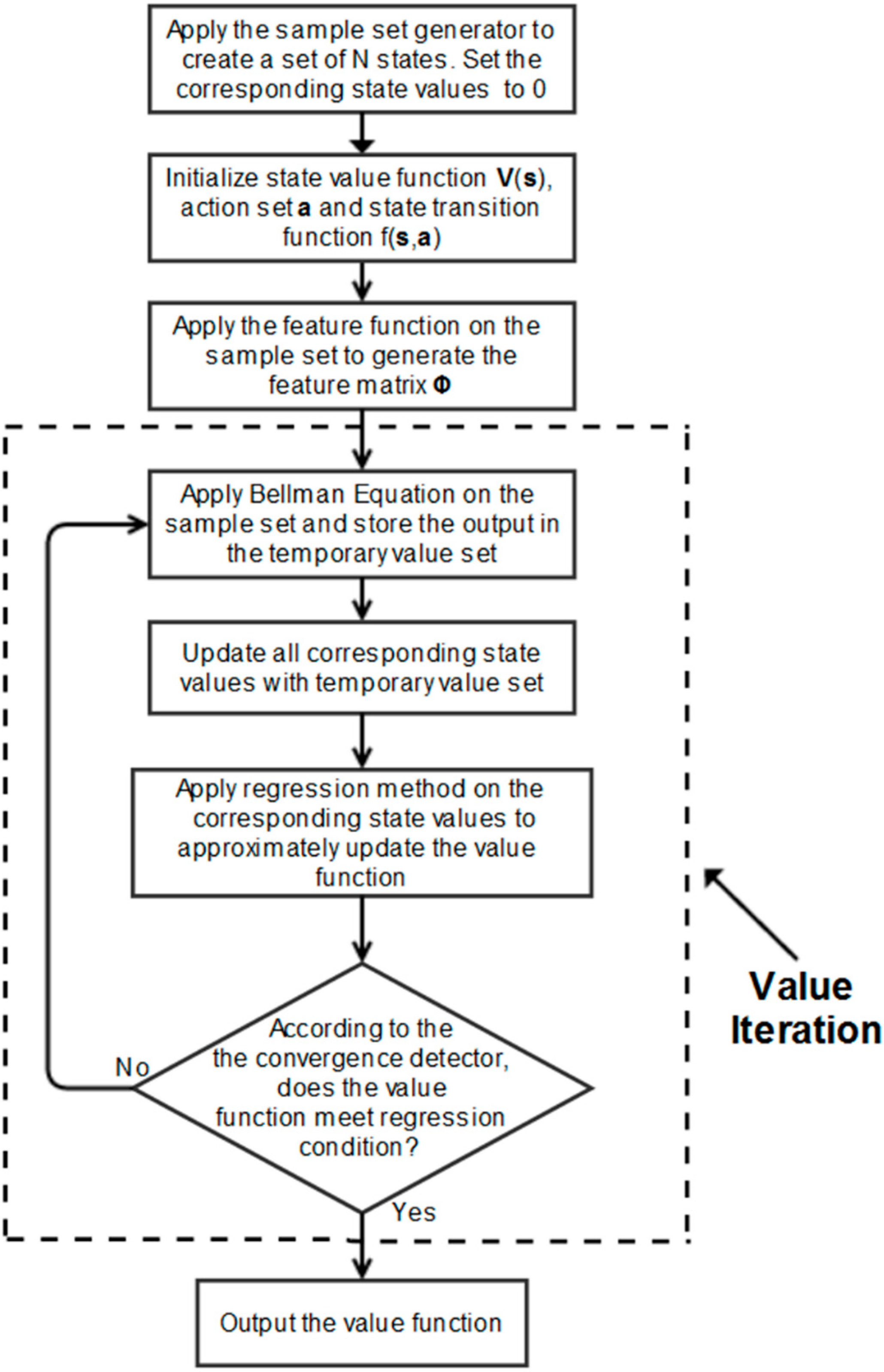
For the non-goal states, their value depends on their reward and a discounted value of the best following state. As this is initially unknown, the non-goal state values are initialized to zero before the value iteration process commences. The value iteration for a discrete space is presented in Equation (13), which is commonly referred to as a Bellman equation.

$$V^{k+1}(s)=T{V}^k(s)=\underset{a}{\arg \max }[\text{γ}{V}^k(f(s,a))+R(s)]$$

(13)

where s is a state vector, T is a Bellman operator, V^k(s) is the value of state s in the k-th iteration, a is the action set, f(s,a) is the transition function and its output is a following state of s found in accordance with the action a. R(s) is the reward function. At each iteration, the state values are updated. In two-dimensional discrete systems, this update rule is iterated for all states until it converges. Then, the value of each state is recorded in a lookup table. However, in the simulation, the state-space is multi-dimensional and continuous, so a continuous value function is needed to determine the state value. Hence, a regression mechanism is used to approximate the value function after the value update process completes for each iteration.

With path-planning for multiple agents, the state values cannot simply be recorded in a lookup table because of the continuity and dimensionality of the state-space. The state values need to be represented by a value function. An approximate value function serves as a general scoring scheme for the state-space. A continuous version of the iterative value assignment is used in the simulation. By the end of the learning phase, it is able to provide an approximate score V(s) for any arbitrary state s, which converges to its optimal value V*(s). As it is impractical to find the exact value of each point in multi-dimensional space, a fixed number of states are used as samples to learn the value function, and the method of least squares is also employed for approximation purposes. The iterative process stops when the samples’ value converges.

The state vector itself cannot provide any indication of its value. The features of a state are calculated from the state vector that shapes the value function. The feature vector $\text{φ}\in {\text{R}}^3$ of s is denoted as follows:

$$\text{φ}(s)=[{\text{φ}}_1(s),{\text{φ}}_2(s),{\text{φ}}_3(s)]$$

(14)

Currently, three features are considered for each state. Feature 1 reflects the overall distance to the projected path, which helps vehicles move closer to their goal. The second feature concerns fairness, which aims to evenly distribute the inconvenience of the steering motion. Our aim is to balance the length of the detours that the cooperating vehicles must execute. The last feature reflects the distance between vehicles, which helps to filter out motions that lead to collisions. The definition of each feature is presented in detail in Section 5.

For the approximate value function V(s) to be learned from a sample set $S\in {\text{R}}^{m\times 6}$ of m states, a feature matrix $\Phi \in {\text{R}}^{m\times 3}$ is defined as:

$$\Phi (S)={[\text{φ}(s_1),\text{φ}(s_2),\dots \text{φ}(s_m)]}^T$$

(15)

This is to be used in the regression mechanism. If the collection of corresponding sample state values ${\widehat{V}}^{k+1}\in {\text{R}}^m$ is defined as:

$${\widehat{V}}^{k+1}(S)={[T{V}^k(S_1),T{V}^k(S_2),\dots T{V}^k(S_m)]}^T$$

(16)

then the value function V(s) is updated for each iteration until convergence is achieved using a standard least squares estimation as follows:

$$V^{k+1}(s)=\text{φ}(s)\cdot [{({\Phi }^T\Phi )}^{-1}{\Phi }^T{\widehat{V}}^{k+1}(S)]$$

(17)

The proposed scheme works satisfactorily in two-vehicle scenarios; however, it is also required to work with scenarios comprising more than two vehicles. To describe systems with n vehicles, the size of the sample set S increases to m × 3n, and Equations (9)–(11) are refined as follows:

$$s=[x_1^{pos},y_1^{pos},{\text{θ}}_1,x_2^{pos},y_2^{pos},{\text{θ}}_2,\dots ,x_n^{pos},y_n^{pos},{\text{θ}}_n]\in {\text{R}}^{3n},0\le {\text{θ}}_i<2\text{π}$$

(18)

$$a=[a_1,a_2,\dots ,a_n]\in {\text{R}}^n,-\frac{v_i}{r_i^{\text{min}}}\le a_i\le \frac{v_i}{r_i^{\text{min}}}$$

(19)

$$\begin{gathered} d(s)=[d_{1,2}(s),\dots d_{i,j}(s),\dots d_{n-1,n}(s)]\in {\text{R}}^{n(n-1)/2} \\ {d}_{i,j}(s)=\sqrt{{(x_i^{pos}-x_j^{pos})}^2+{(y_i^{pos}-y_j^{pos})}^2},\exists \forall d_{i,j}(s)\in d(s):d_{i,j}(s)\le d_{\text{min}} \\ i,j=1,2,\dots \hspace{0.17em}n,\hspace{0.17em}\hspace{0.17em}i\ne j \end{gathered}$$

(20)

For example, in four-vehicle scenarios, a state vector s has twelve coordinates, as each group of three represents the position and heading of one vehicle; an action vector a has four coordinates, and each of them represents the action of the corresponding vehicle; as every pair of the four should be checked if they are too close to each other, the d(s) vector is six ($C_4^2$ ) dimensional.

5. Decomposition of the Scheme

This section details the proposed RL scheme, which generally has two phases, referred to as the “learning phase” and the “action phase”. The flow charts of the two phases are provided first; then, components within both phases are discussed and illustrated. Finally, the scheme is validated for a number of test cases.

5.1. Learning Phase

In the learning phase, RL is implemented to learn the nature of the problem by assigning appropriate coefficients to different pre-defined state features. Figure 1 shows how the learning phase operates. As it is impossible to evaluate every state in the state space, a collection of sample states are randomly selected according to some constraints. Then, the state value function is initialized to zero. An action set, state transition function and search function are defined. After that, the feature matrix of the sample states is determined, and RL operates on this data iteratively. Finally, when the convergence criteria are met, the value function is ready to be used in the action phase.

5.1.1. Sample Set Generator

A sample set consists of a suitable number of samples to resemble the likeness of the entire state space. Generally, it should include two kinds of state, states indicating collision(s) and those not indicating collisions, but this is not guaranteed if the samples are generated randomly. Hence, some of them are designated. It is quite clear that the starting and ending states should be free from collisions, so the ending state is included in the sample set. In most cases, a crossover of two paths does not mean a collision; However, if two vehicles are at the crossover point at the same time, it does correspond to a collision. Hence, one state indicating two vehicles at the same crossover point with projected orientations is also taken in the sample set. These are the designated sample states, which guarantee at least both one wanted and unwanted state are present in the sample set. For randomly generated sample states, as it is not likely to see vehicles moving along any edge of the area of interest, samples are randomly generated with a heading constraint in a smaller area centred in the area of interest. The heading constraint is that for each vehicle, the difference between the current heading and projected heading should not exceed 90 degrees, as this would momentarily make the vehicles travel in a reverse direction, which is not desirable. By implementing this constraint in the appropriate parts of the algorithm, vehicles tend to stay “close to projected paths” and unwanted directions are unlikely to appear.

Figure 1. Learning phase flow chart.

Figure 1. Learning phase flow chart.

Figure 2 shows what constitutes the sample set, where a two-vehicle scenario is presented and only five samples are illustrated. If a given scenario comprises n vehicles, each sample state is a 3n dimensional vector. If the sample set consists of m samples, then the sample set’s dimension is an m × 3n matrix. The size of the sample set should be determined carefully to balance computational expense and the quality of the result.

Figure 2. Example sample set.

Figure 2. Example sample set.

5.1.2. Feature Function

Rather than directly operating on a sample set, the value function works on the feature matrix derived from the sample set. For simplicity, three features are considered. Feature 1 is concerned with the “inconvenience”, which reflects the overall distance away from projected paths in which the vehicles are. Feature 2 relates to “fairness”, where the difference between the motion of each vehicle at each step is addressed. Feature 3 reflects the number of collisions suggested by the candidate states. Figure 3 illustrates a three-vehicle scenario and the parameters used to calculate the three features for one sample state. In the figure, properties of different vehicles are colour coded. Each round dot stands for a vehicle’s position; solid lines represent projected paths; thick arrows mark the start points and projected directions; and a thin arrow indicates a vehicle’s current direction. h_i is vehicle i’s perpendicular distance from its projected path. a_i is the difference between vehicle i’s current orientation and its projected one in the anti-clockwise direction. d_{i, j} is the distance between vehicle i and vehicle j.

Figure 3. Feature Illustration.

Figure 3. Feature Illustration.

Equation (21) shows how one state is mapped onto its feature vector. c₁, c₂ and c₃ are three positive parameters to tune the function with respect to the order of importance of the features. k is a large integer that ensures that the sigmoid function in φ₃ is sensitive enough to determine collision states. d_min is the minimum distance allowed between any two vehicles. If a sample set consists of m sample states, its feature matrix Φ is an m × 3n one, where n is the number of vehicles.

$$\begin{array}{l}Feature\_Function:\\ s=[x_1^{pos},y_1^{pos},{\text{θ}}_1,x_2^{pos},y_2^{pos},{\text{θ}}_2,\dots ,x_n^{pos},y_n^{pos},{\text{θ}}_n]\\ \to \text{φ}=[{\text{φ}}_1,{\text{φ}}_2,{\text{φ}}_3]\\ {\text{φ}}_1=c_1\cdot {\displaystyle \sum }_{i=1}^n{h}_i\\ {\text{φ}}_2=c_2\cdot \sqrt{\frac{1}{n}{\displaystyle \sum }_{i=1}^n{({\text{α}}_i-\text{μ})}^2},\hspace{0.17em}\text{where}\hspace{0.17em}\text{μ}=\frac{1}{n}{\displaystyle \sum }_{i=1}^n{\text{α}}_i\\ {\text{φ}}_3=c_3\cdot {\displaystyle \sum }_{i=2}^n{\displaystyle \sum }_{j=1}^{i-1}(\frac{1}{e^{k*(d_{\text{min}}-d_{i,j})}}-1)\end{array}$$

(21)

5.1.3. Transit Function

As shown in Equation (22), given a current state and current action, the action function determines the next state.

$$s_{t+1}=f(s_t,a_t)$$

(22)

Given Equation (19) in Section 4, if the action chosen for vehicle i suggests turning a degrees (a ≠ 0) in the anti-clockwise direction and it travels at a constant speed, its position and heading at the next step can be calculated as illustrated in Figure 4, obtained from the equations as follows:

$$\begin{array}{l}{x}_{i,t+1}^{pos}=\frac{2v_i}{a_i}*\text{sin}\frac{a_{i,t}}{2}*\text{cos}({\text{θ}}_{i,t}+\frac{a_{i,t}}{2})+x_{i,t}^{pos}\\ y_{i,t+1}^{pos}=\frac{2v_i}{a_i}*\text{sin}\frac{a_{i,t}}{2}*\text{sin}({\text{θ}}_{i,t}+\frac{a_{i,t}}{2})+y_{i,t}^{pos}\\ {\text{θ}}_{i,t+1}={\text{θ}}_{i,t}+a_{i,t}\end{array}$$

(23)

If the action proposing to go straight ahead is chosen for vehicle i and it travels at a constant speed, its position and heading at the next step can be calculated as:

$$\begin{array}{l}{x}_{i,t+1}^{pos}=v_i*\text{cos}{\text{θ}}_{i,t}+x_{i,t}^{pos}\\ y_{i,t+1}^{pos}=v_i*\text{sin}{\text{θ}}_{i,t}+y_{i,t}^{pos}\\ {\text{θ}}_{i,t+1}={\text{θ}}_{i,t}\end{array}$$

(24)

As all sample states are not close to the edges of the area of interest, the positions produced by Equations (23) and (24) will not be outside the area of interest, whereas headings need to be selected in the defined field [0, 2π).

Figure 4. Generating the arc path.

Figure 4. Generating the arc path.

5.1.4. Search Function

The search function determines the best action from the current state by evaluating the value of all possible next states while the value function V(s) is updated in parallel. As the state space is multi-dimensional and continuous, it is impossible to traverse every potential next state. Figure 5 gives the pseudo code for the search function. This algorithm features a binary search to reduce complexity.

Figure 5. Continuous action search algorithm.

Figure 5. Continuous action search algorithm.

5.1.5. Iterative Update Function

The value function V(s) is initialized as zero and iteratively updated until convergence and can be expressed as the weighted sum of feature components:

$$V(s)=\text{β}\cdot \text{φ}{(s)}^T,where\text{β}\in {\text{R}}^3$$

(25)

Since φ(s) is determined when designing the feature function, it is the β vector that is updated iteratively.

As suggested in Equation (17) in Section 4, in each iteration, β for the next iteration is obtained using the least squares method as:

$${\text{β}}^{k+1}={({\Phi }^T\Phi )}^{-1}{\Phi }^T{\widehat{V}}^{k+1}(S)$$

(26)

where k denotes the current iteration, ${\widehat{V}}^{k+1}(S)$ is obtained as the sample value by applying V(s) of the current iteration in the Bellman Equation (Equation (13)).

$$V^{k+1}(s)=T{V}^k(s)=\underset{a}{\text{arg} \text{max}}[\text{γ}{V}^k(f(s,a))+R(s)]$$

(27)

5.1.6. Convergence Detector

The convergence detector determines when to stop value iteration and enter the action phase by comparing the magnitude of the difference between the value samples of the last two iterations. Its pseudo code is shown in Figure 6.

Figure 6. Pseudo code of convergence detector.

Figure 6. Pseudo code of convergence detector.

Figure 7 shows three examples of how the sample state value variations diminish until convergence is reached for several simulations of the same test case. In each simulation, when for all states in the sample set, there is only minor value variation between iterations, convergence is assumed to have taken place. As shown in Figure 7, the mean squared error (MSE) of the approximate value of sample states between iterations is used to indicate if the approximate value function has converged to an acceptable standard, where the possible minor improvement in the next iteration will no longer affect the transition decision from any state. We find that, if convergence is to take place, it generally occurs within relatively few iterations. Therefore, rather than let the simulation proceed for many iterations, it is more appropriate to halt the progress after a fixed iteration count if convergence has not taken place and restart the evaluation with a different set of seeds. For the results given in Section 7, we allow for 16 repeats of the learning phase before declaring a failure to find an adequate solution. At that point in time, we could resort to one of the non-cooperative simple collision-avoidance schemes as a failsafe, though this situation rarely arises.

Figure 7. Example of convergence.

Figure 7. Example of convergence.

5.2. Action Phase

Figure 8 provides a flow chart of the action phase, where the system uses the value function generated during the learning phase to determine the paths. When the ending criteria for either successful or unsuccessful planning cases are met, the action phase is concluded.

The value function obtained from the learning phase is used in the action phase to determine the state transition for each step, where the same transit function, search function and feature function are invoked as used in the learning phase. Though the RL approach is generally very good at finding suitable detour paths, it is still possible to experience a “deadlock” situation when planning the paths. By this, we mean the search function has led the system into a local extremum next to forbidden states in the state space, which indicates no action is able to avoid a collision. To resolve this, an action phase backup strategy can be invoked, as described in Section 5.2.1.

5.2.1. Backup Scheme

Due to the deterministic nature of the RL model employed in the learning phase, it is possible that sometimes the value function and search function can lead the system to an unwanted state where no valid next state is available. Hence, a backup scheme is needed to permit backtracking in the planning phase. A one-step backup scheme is currently implemented as shown in Figure 8. If during the path-planning no valid next state is encountered, the algorithm backs up to the preceding state and selects the next state with the lowest value amongst all of the valid next states available. This state is chosen, as it is the most different valid choice from the one that previously led to the invalid next-state condition.

5.2.2. Ending Criteria

Vehicles are required to return to their projected paths smoothly rather than to re-join the path obliquely. However, when all vehicles are travelling on their projected paths, it does not mean that the action phase has ended. There are chances that vehicles might veer away again after re-joining their projected paths.

Two mutually exclusive ending criteria are considered. If the system meets either of them, the action phase terminates. The first one is that all vehicles have left the area of interest. If this criterion is met, the ending positions of all vehicles will be checked to see if they returned to their projected paths or not. The second one is that the action phase has proceeded for a limited number of steps. Meeting this criterion means the other one is not fulfilled, such that vehicle(s) have spent too long in the area of interest. This situation can arise when a series of detours is generated in response to a succession of collision domain avoidance events.

Figure 8. Action phase flow chart.

Figure 8. Action phase flow chart.

6. Validation

The proposed scheme is designed to perform collision avoidance between multiple moving cooperative vehicles. However, due to its versatility, it can also be used in scenarios with stationary obstacles. Obstacles can be regarded as cooperative vehicles with a zero velocity and zero effect on the state transition. The proposed scheme is implemented in MATLAB and functions appropriately with challenging test cases as expected. A variety of scenarios with two, three and four homogeneous vehicles are examined, and typical results are as shown in Figure 9. As shown in the results, due to its cooperative nature, vehicles can avoid collisions whilst experiencing minor inconvenience distributed fairly.

Figure 9. Validation results.

Figure 9. Validation results.

7. Performance Assessment

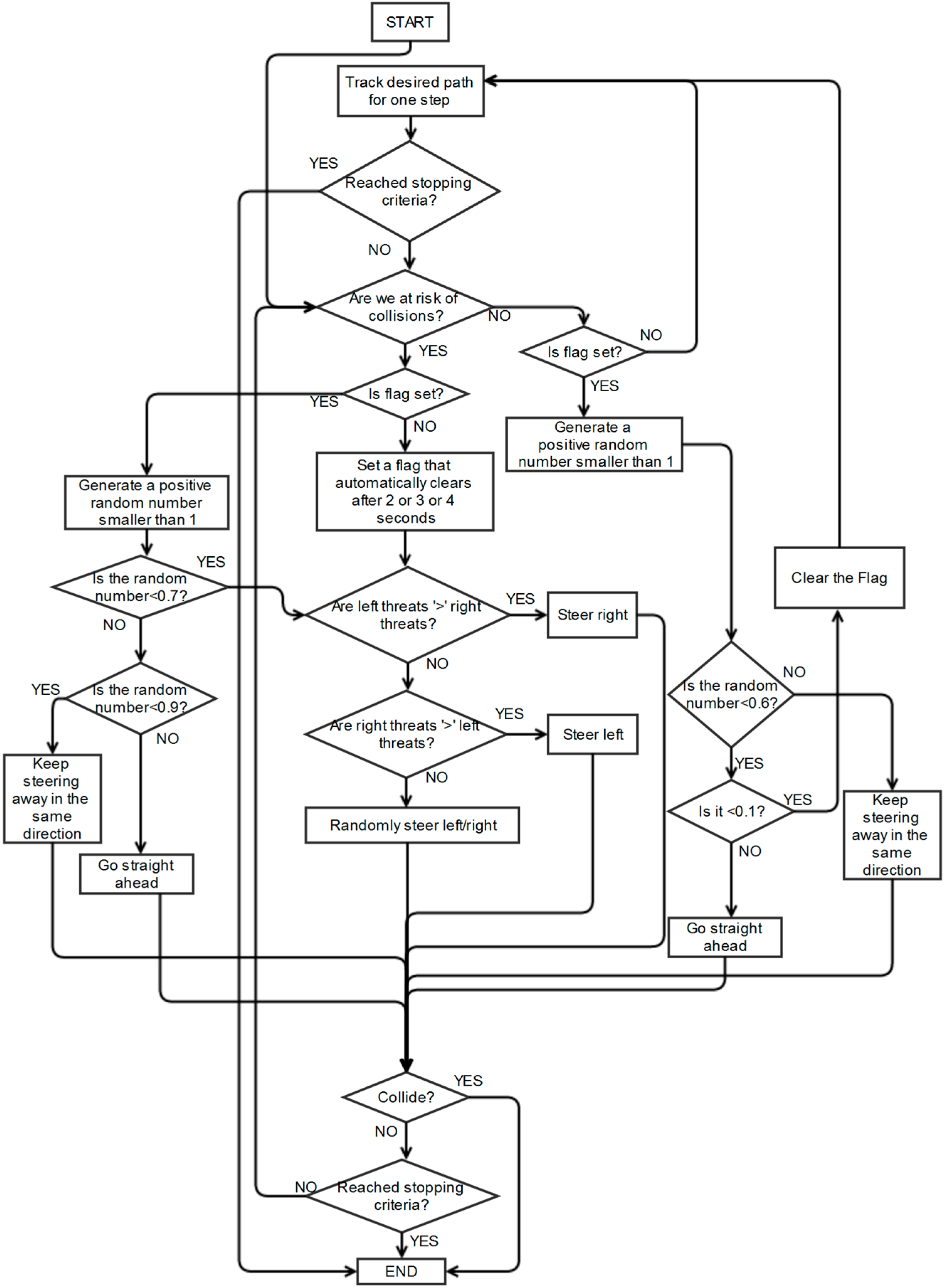
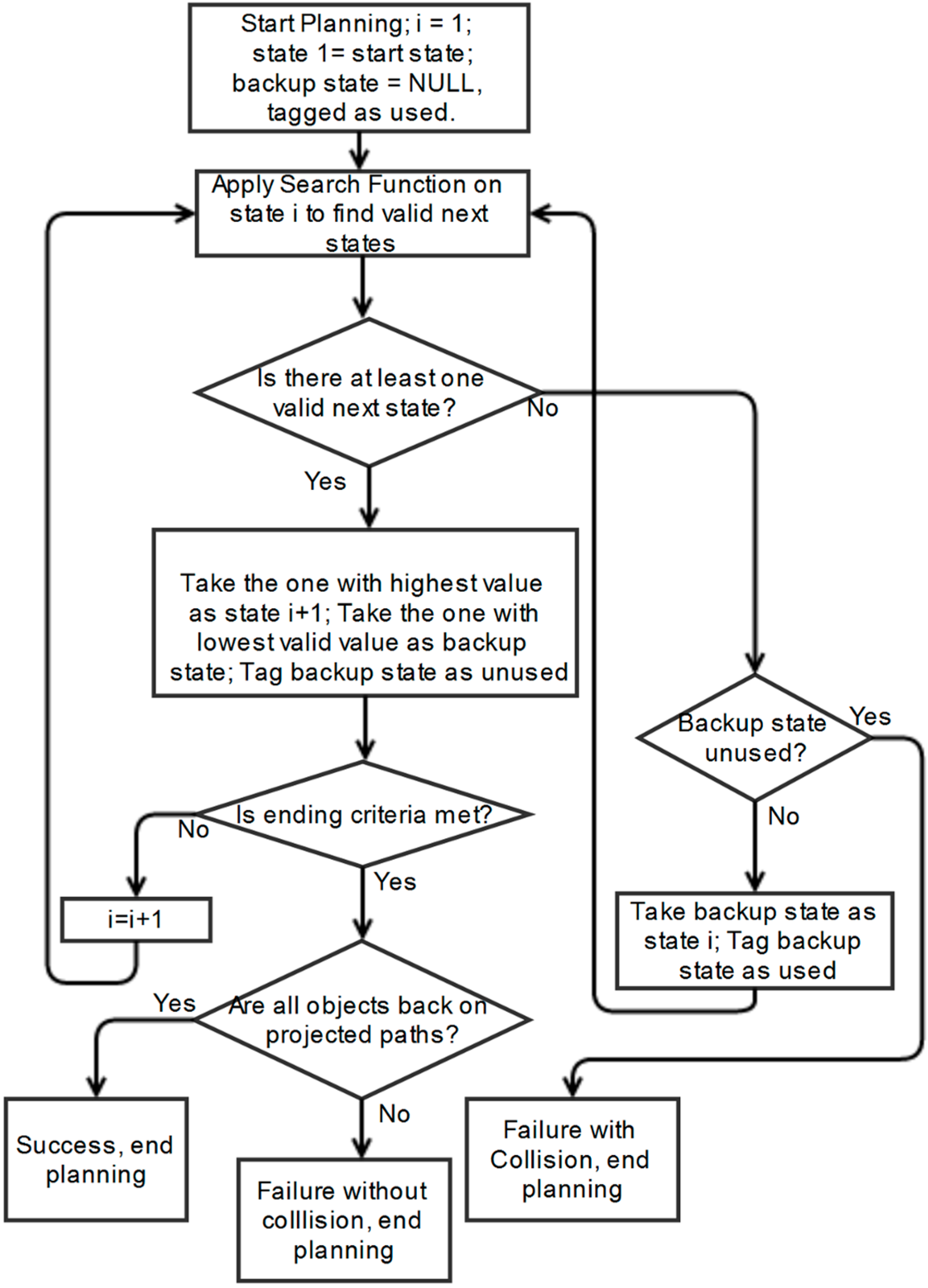
As there is no scheme in literature with similar assumptions and requirements to the one we propose, we create two alternative schemes to form a baseline comparison. Firstly, a simple scheme is presented. Its flow chart is shown in Figure 10.

Figure 10. Flow chart of original simple scheme and illustration of pathological synchronized motion.

Figure 10. Flow chart of original simple scheme and illustration of pathological synchronized motion.

The scheme is for vehicle(s) that make their own steering decisions without communication with other vehicles. The judgment of the risk of collision is based on the velocity-obstacle method described in [43]. If all vehicles use this simple scheme to plan paths, it is possible that some potentially colliding vehicles can enter synchronized motion, because they make decisions in a similar fixed manner. This can lead to endless reoccurring patterns of behaviour between them once they decide to steer back onto their original path, as illustrated in Figure 10. Hence, a modified scheme is introduced to decrease the chances of vehicles repeating synchronized motions. It employs a random number generator in the decision process to differentiate their motions, as illustrated in Figure 11.

Figure 11. Flow chart of the modified simple scheme.

Figure 11. Flow chart of the modified simple scheme.

In the subsequent simulations, each vehicle travels at 20 m per second with a maximum angular speed of 45°/s and has a clearance area with a radius of 22.5 m, so d_min from Equation (21) is 45 m. Test cases are constructed featuring a two-dimensional square area of interest with side edges of 500 m. The start points of vehicles are on the boundaries of the area. The goal is successful collision avoidance within the area of interest. For the RL scheme, based on experience with repeatable trails, the design parameters are set as follows: c₁, c₂, c₃ are set to 0.006, 0.012 and 1, respectively. These weightings are to normalize the importance of each feature. 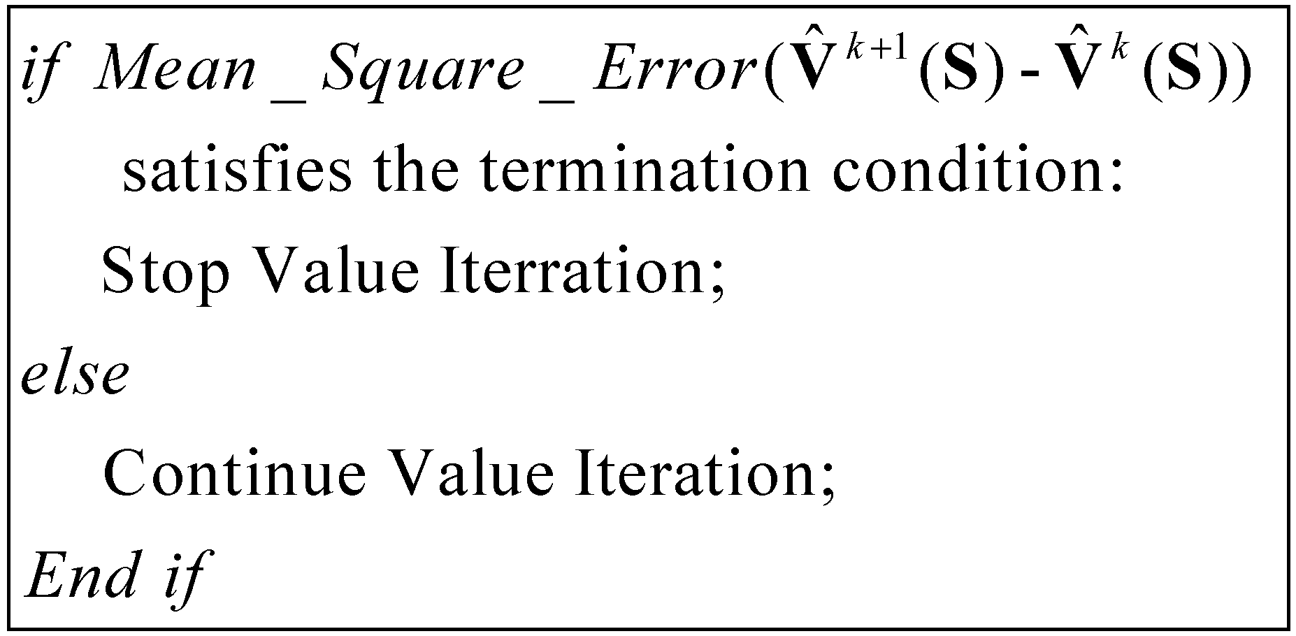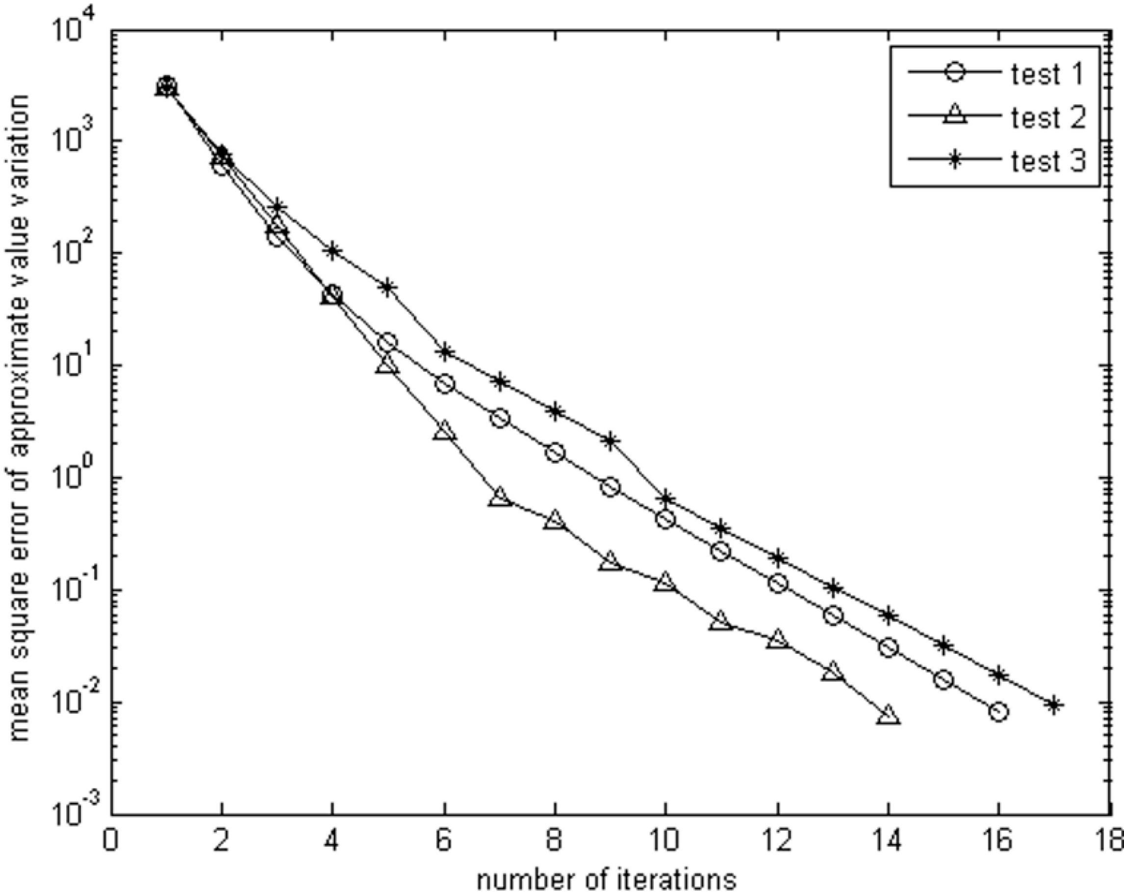k is initialised to 2000; the discount factor γ is set to 0.9; the reward is 100 for goal states, −100 is assigned to forbidden states and −5 for other states; convergence is considered to have taken place when the mean squared error referred to in Figure 6 is smaller than 0.01.

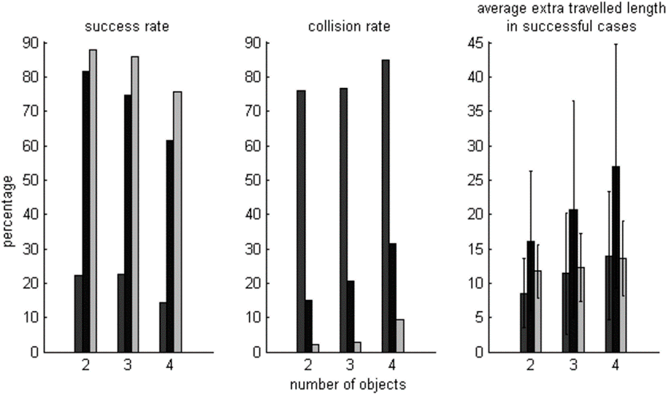
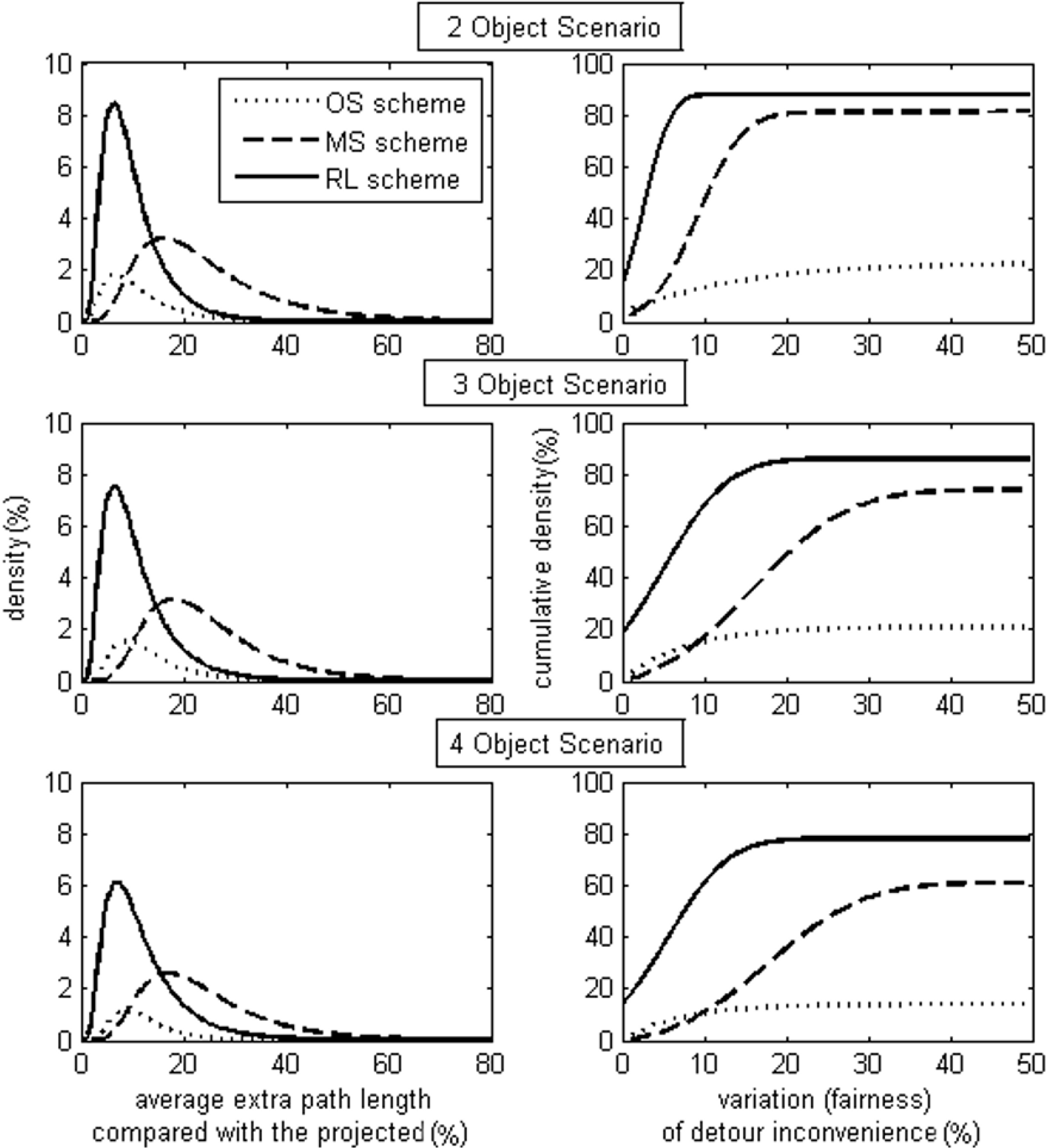
Statistical results, collected from 2000 different trials with potential collision(s), are presented in Figure 12 and Figure 13. Results for the extra distance travelled (i.e., the detour length) are only shown for successful collision avoidance cases. In all instances, figures shown on the Y-axis are percentages. For example, as shown in Figure 12, the success rate of the original simple scheme for two-vehicle scenarios is about 22%, and the distribution results of the two-vehicle scenarios shown in Figure 13 are based on those 22% successful cases.

Figure 12. Comparison between schemes (Part I).

Figure 12. Comparison between schemes (Part I).

Figure 13. Comparison between schemes (Part II).

Figure 13. Comparison between schemes (Part II).

The original simple (OS) scheme takes the most obvious action to avoid collisions and returns to desired paths as soon as it realizes it is within a collision domain. However, all vehicles behave in the same way, so that there is a high risk of either experiencing a collision or pursuing oscillatory paths after steering back, which leads to a low success rate and high collision rate. For example, in the two-vehicle scenario, the success rate is only about 21%, although in these successful cases, less than 10% more distance is traversed. As suggested from the results of the success rate density distribution against average detour inconvenience, longer detour paths do not arise often. With the OS scheme, it either finds a simple collision avoidance solution traversing a small detour distance or it enters a pathological series of collision avoidance steps that result in deadlock. As the results of a four-vehicle scenario show in Figure 13, it is almost impossible to expect the OS scheme to solve problems with more than 25% extra distance. OS is a solitary decision making scheme, where vehicles only take evasive action to deal with the imminent threat of a collision without considering the possibility of subsequent collisions with vehicles not necessarily involved in the current threat. Thus, the more vehicles that are present in the area of interest, the less fairly the OS scheme works. This can be seen from the three plots featuring the cumulative success rate against deviation of detour inconvenience in Figure 13. In the two-vehicle scenario, there is about a 6% success rate with zero deviation, and in the three and four-vehicle scenarios, the success rate drops to zero.

The modified simple (MS) scheme shows better performance than the OS scheme in terms of success rate and collision rate. As it has a mechanism to randomly influence the decisions vehicles make. Thus, it is unlikely for vehicles to remain synchronized when detouring away from or returning to desired paths. However, the MS scheme is less likely to provide straightforward solutions, and consequently, it typically results in a greater detour distance being travelled. For example, in successful cases of two-vehicle scenarios, as shown in Figure 12, the average distance traversed with the MS scheme is almost twice that of the OS scheme. This is, in part, because decisions are made randomly, so there is a lower possibility of fairness amongst the vehicles. For example, as shown in the plot featuring the cumulative success rate against deviation of detour inconvenience for the three scenarios in Figure 13, on the left-hand side, the dotted curves are above the dash-dot ones, which means that the MS scheme provides fewer solutions with little unfairness than the OS scheme. Furthermore, compared with the solid curves, the dash-dot ones are of a more gradual slope, which means in the case of the RL scheme, the distribution of detour unfairness results are clustered around lower percentage values (i.e., towards the left-hand side of the graph) showing that the scheme provides a reasonable degree of fairness. Conversely, the MS scheme shows results evenly scattered along the horizontal axis, showing that in many cases, there is considerable imbalance/unfairness between the detour paths taken.

From Figure 12, for the scenarios considered, the RL scheme provides the greatest success rate and lowest collision rate with an acceptable level of detour inconvenience. For example, in the four-vehicle scenario, the success rate of the RL scheme is 10% higher than that of the MS scheme, while its collision rate is more than 60% lower and the detour inconvenience is 50% less. From the three plots on the left of Figure 13, the RL solutions are seen to be more condensed to a lower degree of detour inconvenience. Additionally, from the three plots on the right-hand side of Figure 13, the solid curve, representing RL, has a much greater slope at the beginning and starts with a much higher success rate than the others. For example, in the three-vehicle scenario, the success rate with complete fairness with the RL scheme is 21%, whilst those of the other schemes are zero. As detour inconvenience and fairness are taken into account in the RL scheme, its solutions provide the shortest extra travelled distance, the greatest success rate and the greatest fairness amongst three schemes, and vehicles are more likely to take the shortest possible detour paths, as expected.

8. Conclusions

In this paper, the problem of collision avoidance in multiple-vehicle systems is considered under constant speed requirements. A reinforcement learning approach is proposed as a fast acting online scheme. This is particularly beneficial in dynamic environments where new vehicles may stray into the area of interest at any point in time.

The main motivation of this research has been to plan collision avoidance paths in a cooperative, fair and efficient manner. The proposed scheme considers the problem as a decision process comprising a learning phase and an action phase. In the learning phase, reinforcement learning is implemented to develop a value function from a set of state samples, which reflects the likelihood of successfully reaching the goal state from a given state. In the action phase, the system makes use of the value function to plan paths for all vehicles. The proposed scheme performs satisfactorily in scenarios with or without a single stationary obstacle. Simulation results show that the proposed scheme is computationally simple enough to be employed online, requiring few iterations to converge on a reasonable solution. As there is no other relevant research with similar assumptions and requirements, two alternative schemes are proposed to function as benchmarks. Compared with these non-cooperating alternatives, the RL scheme shows significant benefit in terms of path efficiency, fairness and success rate.