Article

Feature Selection and Fault Detection Under Dynamic Conditions of Chiller Systems

Department of Building, Civil and Environmental Engineering, Concordia University, Montreal, QC H3G 1M8, Canada
*
Author to whom correspondence should be addressed.
Electronics 2026, 15(1), 208; https://doi.org/10.3390/electronics15010208 (registering DOI)
Submission received: 5 November 2025 / Revised: 16 December 2025 / Accepted: 20 December 2025 / Published: 1 January 2026

Abstract

Faults in chiller systems can significantly reduce energy efficiency and operational performance. To address this, fault detection and diagnosis (FDD) algorithms are increasingly integrated into building management systems (BMS). This study proposes a comprehensive FDD framework addressing two key aspects: (1) fault detection under dynamic operating conditions and (2) selection of key variables for unsupervised fault detection. Traditional approaches usually assume steady-state operation, limiting their ability to capture transient and nonlinear system behaviors. The proposed method integrates Variational Mode Decomposition (VMD) for noise reduction and signal denoising with Kernel Principal Component Analysis (KPCA) to capture nonlinear behavior in chiller systems. This combination enables accurate fault detection under both steady and transient conditions. Furthermore, a wrapper-based step-forward feature selection algorithm identifies the most informative variables for KPCA-based fault detection. Assuming at least one known fault type, the method minimizes the Missing Alarm Rate (MAR) and False Alarm Rate (FAR), enhancing adaptability to different sensor configurations. The proposed approach is validated on the ASHRAE RP-1043 dataset using first-level severity faults. Results show that the VMD-KPCA method detects 98% of faulty samples, significantly outperforming linear PCA (55%), and highlight the importance of vapor compression parameters and thermodynamic insights in improving fault detection reliability.

1. Introduction

Chiller systems are one of the main components of Heating, Ventilation, and Air Conditioning (HVAC) systems and are mainly used for cooling purposes in commercial buildings [1]. They are among the most energy-intensive components, often accounting for up to half of a building’s electricity consumption [2]. A vapor-compression chiller operates using a closed refrigerant cycle that includes four main components: an evaporator, a compressor(s), a condenser, and an expansion device. In the evaporator, the refrigerant absorbs heat from the building’s water loop, producing chilled water. The refrigerant vapor is then compressed and delivered to the condenser, where it rejects the absorbed heat either to outdoor air (air-cooled chillers) or to a condenser water loop connected to a cooling tower (water-cooled chillers), as demonstrated in Figure 1. After passing through the expansion device, the refrigerant pressure and temperature decrease, allowing it to re-enter the evaporator and repeat the cycle [3]. In addition to this basic cycle, modern chillers often include various auxiliary components to improve efficiency, stability, and safety. Depending on the design, these may include an economizer, expansion turbine, subcooler, lubricant cooler, lubricant separator, lubricant-return mechanism, purge unit, lubricant pump, refrigerant transfer equipment, refrigerant venting devices, and additional control valves [4]. These auxiliary subsystems support reliable operation, enhance part-load performance, and expand the chiller’s overall capabilities.
In terms of operation, chiller systems operate under two primary time regimes: steady-state and transient conditions. In steady-state operation, the key variables remain relatively stable, whereas in transient operation, the system is undergoing change over time. Transients in chiller systems arise from several phenomena, including start-up and shutdown processes, ramping of compressor speed, refrigerant phase-change dynamics inside heat exchangers, and fluctuations in building load [5]. When the system operates long enough near a defined setpoint, and the variables exhibit minimal variation, it is considered to be in steady state. To distinguish these regimes, steady-state detection techniques typically evaluate the rate of change (slope) or statistical variation (e.g., standard deviation) of measured variables over time. A slope approaching zero or a small variance indicates steady-state behavior, whereas higher rates of change signify transient operation. Various methods in the HVAC literature combine these criteria to robustly identify steady-state and transient periods [6].
Given various components involved in chiller systems and vapor compression systems, along with the high cost of these components, various time regimes and behaviors, and the significant energy demand of chillers, effective control strategies, energy-efficient operation, and regular maintenance are essential to ensure reliable performance and prevent failures [6,7].
Fault Detection and Diagnosis (FDD) is a method that enables continuous monitoring of chiller performance, allowing for the identification of faults or failures that could lead to energy inefficiency and adverse environmental impacts [8]. According to some studies, detecting and diagnosing faults in HVAC systems and rectifying them can lead to energy savings of 20–30%, highlighting the importance of FDD implementation [9]. Modern FDD can be categorized into three main methods, i.e., quantitative model-based (physics-based or White box models), qualitative model-based (knowledge-based), and process history-based (Data-Driven and gray box) [10].
Developing physics-based and rule-based models requires a deep understanding of the underlying physics and governing equations [11]. However, these methods often fall short when dealing with complex systems, such as large chiller systems with multiple components. For instance, accurately modeling such systems is challenging due to the need to account for numerous parameters that may not always be available [12]. Due to these challenges, data-driven techniques have recently gained popularity due to the availability of extensive data, their effectiveness in pattern recognition, and their ease of developing and capturing nonlinear patterns without requiring an in-depth understanding of the physical laws governing chiller systems [13].
Data-driven techniques generally fall into two categories: supervised and unsupervised methods [14,15]. Supervised approaches typically require both faulty and fault-free data for detection and diagnosis. However, in real operational environments, fault labels are scarce, expensive to obtain, and often unavailable, whereas normal operating data are abundant [16] While the current study focuses on unsupervised fault detection within a single system, this challenge also motivated recent work on transfer-learning strategies in the broader HVAC fault diagnosis literature, where labeled data from a source domain, constructed through simulation or domain knowledge, is used to guide diagnosis in a target system with limited labels [17]. In parallel, unsupervised approaches remain highly practical, especially for fault detection, as they rely solely on the abundant fault-free operational data available in the chiller systems [18].
In unsupervised fault detection methods, such as Principal Component Analysis (PCA), it is common practice to establish a baseline for the chiller system. This process involves identifying the system’s normal behavior and developing a model to represent it [19]. The model is then applied to new measurements to detect any deviations from the fault-free baseline.
There are several challenges and limitations associated with PCA. Many studies highlight that because PCA is a linear transformation method, its performance in detecting faults can be degraded due to the inherently nonlinear behavior of chiller variables [20]. Much of the nonlinearity in chiller systems arises from transient conditions and dynamic processes in the Vapor Compression Cycle (VCC), such as the phase changes of refrigerant in heat exchangers and fluctuations in building load [5]. To reduce the complexity of analysis using PCA and its extension methods, many studies excluded the transient behavior of the chiller system [21,22]. However, by removing the transient behavior, the nonlinearity of the system that they highlighted is reduced to some extent.
The other challenge is detecting faults in the early stages and at low severity levels. Detecting incipient faults is critical to preventing significant energy and economic losses in chiller systems [23]. However, some studies have shown that faults like refrigerant leakage (RL) have a negligible impact on overall performance in their early stages, even when models are developed for steady-state conditions [24]. In contrast, other studies indicated that such faults can be more effectively identified during transient conditions, such as system start-up, indicating that some faults are sensitive to time regimes, and leveraging different time regimes of the system can enable easier and quicker fault detection [25].
While developing a robust FDD algorithm is essential, the selection of variables that are highly sensitive to faults plays a critical role in the model’s success [26]. In addition to enhancing FDD performance, selecting an optimal number of features helps eliminate redundancy within the dataset, thereby reducing the computational complexity of the FDD model [27]. Furthermore, minimizing the number of features directly reduces the need for sensor installations, leading to lower costs associated with sensor deployment and maintenance [28]
The above-discussed challenges underscore the need for a fault detection framework capable of addressing these issues, which include developing an unsupervised algorithm that can operate effectively under the dynamic and transient conditions of chillers, as they often function across varying time regimes and may not consistently reach steady-state, rendering traditional steady-state-based models inadequate for reliable fault detection [25,29]. Moreover, transient operating periods can contain valuable information that enables earlier and more accurate fault identification, as reported in several studies [25]. In addition, identifying the key variables most relevant to unsupervised fault detection under both steady and transient conditions remains an open challenge that requires further investigation.
Therefore, this study focuses on two main contributions through the development of the following methods:
(1)
An unsupervised fault detection algorithm is developed for chiller systems operating under dynamic conditions. The approach consists of two main components: (i) a denoising stage using Variational Mode Decomposition (VMD) to isolate dominant signal modes and (ii) a detection stage using Kernel Principal Component Analysis (KPCA) to capture nonlinear system behavior and identify deviations indicative of faults under both steady-state and transient operating conditions.
(2)
A wrapper-based forward selection (FS) method is employed to identify the key variables that remain sensitive to faults under dynamic operating conditions for the unsupervised VMD-KPCA framework, improving detection accuracy and reducing false alarm rates while enabling the use of a reduced sensor subset when certain measurements are missing or unavailable in the chiller systems.
The remainder of this paper is organized as follows. Section 2 presents a review of relevant literature, covering denoising techniques, Principal Component Analysis (PCA) and its extensions, as well as feature selection methods, with key research gaps highlighted at the end of each subsection. Section 3 describes the proposed methodology, including the VMD-KPCA fault detection framework and the feature selection strategy. Section 4 reports and analyzes the experimental results. Finally, Section 5 concludes the study and outlines potential directions for future research.

2. Literature Review

This section reviews the key research on fault detection and feature selection methods for chiller systems. The first part focuses on research that applied signal decomposition methods and PCA, different variants of PCA, and a hybrid of PCA with other techniques to detect faults in HVAC systems, with an emphasis on chiller systems. The second part examines studies that developed methods for feature selection.

2.1. Denoising Data Through Signal Decomposition Methods for FDD Using PCA

To improve PCA performance and deal with the dynamic behavior of the HVAC systems, some studies adopted signal processing methods to decompose the data and remove noise, including wavelet transform and Empirical Mode Decomposition (EMD).
Xu et al. [30] improved chiller sensor FDD by combining wavelet analysis with PCA. While the wavelet analysis reduced noise and dynamic effects, a steady-state filter was also adopted to remove transient behavior. Although the wavelet–PCA method outperformed standard PCA, it had difficulty detecting low-level bias faults in evaporator and condenser pressure. Li and Wen [31] proposed a hybrid fault detection method using wavelet transform and PCA for AHUs. The wavelet transforms initially removed high-frequency noise and then iteratively decomposed the low-frequency components, isolating the detrended signal to train the PCA model. While validated on three fault types, the method failed to detect a leaking heating coil valve and did not address other faults specified in ASHRAE 1213. Mao et al. [32] combined Empirical Mode Decomposition (EMD) with PCA to detect sensor bias faults in chillers. EMD handled dynamic behavior and reduced noise by decomposing data into high- and low-frequency components, where a threshold technique filtered noise from the high-frequency data. The cleaned data was then reconstructed for PCA. Li and Hu [33] applied Ensemble Empirical Mode Decomposition (EEMD) to denoise data before using PCA for the detection of sensor faults in chiller systems. While the EEMD-PCA method slightly outperformed standard PCA, it struggled to detect sensor faults at lower bias levels.
The reviewed studies indicate that previous research has primarily focused on applying signal decomposition techniques for sensor fault detection in chillers and air handling units (AHUs), while their application for component-level fault detection in chillers remains unexplored. Moreover, the signal decomposition techniques used, such as Wavelet and EEMD, have certain limitations. The wavelet transform’s effectiveness depends on the choice of wavelet function and decomposition level, and it may struggle with complex dynamics due to reliance on fixed functions [34]. Moreover, EMD, being data-driven, lacks a solid mathematical foundation and is sensitive to noise and sampling [35].

2.2. PCA and Hybrid of PCA Methods for Steady-State FDD

In addition to enhancing PCA performance through noise reduction and the management of dynamic behavior, several studies have improved fault detection by addressing transient behaviors, integrating PCA with other techniques, and employing various types of PCA. The following section reviews studies that specifically tackle the nonlinear behaviors of chillers, while additional studies are summarized in Table 1.
Simmini et al. [37] introduced a local PCA approach to address chiller nonlinear behavior, using seven features to detect condenser fouling (CF), evaporator fouling, and compressor degradation in an air-cooled water chiller with steady-state simulation data [36]. In their follow-up study, Simmini et al. [39] developed a Kernel PCA (KPCA) method using a Gaussian kernel function with a self-tuning algorithm. They validated this method on two steady-state benchmark datasets: a simulated chiller dataset (using the same seven features) and the ASHRAE RP-1043 dataset, which utilized seventeen variables. Xia et al. [38] introduced Kernel Entropy Component Analysis (KECA), an extension of PCA, to tackle the non-Gaussian and nonlinear behavior of chiller systems for fault detection in a water-cooled chiller. In their approach, transient data was excluded, and all sixty-four variables measured in ASHRAE RP-1043 were utilized as inputs for KECA. Gao et al. [43] proposed a fault detection method that integrates Independent Component Analysis (ICA). They trained the ICA model using sixteen features under steady-state conditions. For fault diagnosis, the k-nearest neighbor (k-NN) algorithm was employed to isolate specific faults based on the directions of the residual vector. Lu et al. [40] developed a fault detection method that combines Kernel Entropy Component Analysis (KECA) with the Local Outlier Factor (LOF) to enhance accuracy for low-severity faults. They applied KECA to a dataset of sixteen variables and used LOF as the fault detection index, overcoming the limitations of traditional SPE and T2 in handling nonlinear and non-Gaussian measurements. While the method effectively detected early-stage faults, it was tested under steady-state conditions of the chiller system.
The analysis of the reviewed studies reveals several shortcomings in the existing research. Although various PCA methods were employed to address the nonlinear behavior of chiller systems, most studies focused solely on steady-state fault detection, neglecting the system’s transient behavior. Additionally, efforts to detect low-severity faults often fell short, particularly in identifying issues such as refrigerant leakage, even under steady-state conditions. Moreover, while different sets of variables were used for chiller fault detection, no sensitivity analyses were conducted on the number of variables incorporated in the PCA models. For instance, Xia et al. [38] used all 64 variables recorded in the ASHRAE experiment, while some of those features were recorded twice for the sake of accuracy, and some features were recorded specifically for that test.

2.3. Feature Selection Using Machine Learning Models for Chiller FDD

The selection and extraction of features for FDD can be achieved manually or automatically. In the former case, features are extracted and selected based on the experiment, previous knowledge of the system, and thermodynamic relationships, while in the latter case, statistical and machine learning approaches are employed to choose the most important variables for FDD [44]. Automatic feature selection and extraction are classified as Filter, Embedded, and Wrapper methods [45]
Several studies in the literature have focused on identifying key variables essential for fault detection and diagnosis. The following section reviews these studies and illustrates the features selected by each using machine learning models in Table 2.
Han et al. [46] developed a method combining filtering and wrapper techniques to identify key features for chiller fault detection. They assessed variable correlations using mutual information and used a Genetic Algorithm (GA) to select features for training a Support Vector Machine (SVM) model, achieving a classification accuracy of 99% with eight to thirteen variables related to the evaporator and condenser. Yan et al. [28] introduced a back-tracing sequential forward feature selection (BT-SFS) algorithm for chiller fault detection that incorporates cost-sensitive learning. By integrating a cost-sensitive classification definition into the SVM classifier, the method prioritizes and selects an optimal set of eight to sixteen features based on their importance. Gao et al. proposed a multi-layered approach for chiller fault detection feature selection that combines Random Forest (RF) and global sensitivity analysis using the Sobol method to calculate sensitivity indices. They applied a three-step cascade feature cleaning process to eliminate complex features, resulting in two subsets of fourteen and nine variables, which achieved the highest diagnostic accuracy [47]. Wang et al. [48] emphasized practical feature selection for fault detection, categorizing variables into commonly available, less common, and experiment-specific groups. They developed an initial feature library through a three-step process that included identifying sensors from chiller manufacturers, cost analysis, and thermodynamic evaluation, resulting in feature sets of thirteen, twenty-six, and forty-two variables. Using a Genetic Algorithm–Bayesian Network (GA-BN) as the primary model, they achieved the highest accuracy with six, eight, and ten features from the respective cases. Bi et al. [49] proposed a feature selection approach that ranks the top ten features by combining SHAP analysis with Normalized Feature Weight Calculation (NFWC) across four machine learning models: Random Forest (RF), XGBoost, LightGBM, and CatBoost. Their combined results identified thirteen unique features, which were refined to ten using Pearson’s correlation analysis. While the study addressed both steady and transient states of the chiller system, it did not explore the physical interpretability of the selected features or their influence by system faults, as highlighted in their studies.
The only study that investigated important variables for fault detection using an unsupervised PCA method for chiller systems was conducted by Bezyan et al. This study focused solely on the steady-state behavior of the chiller system and identified 13 key features from 64 variables. However, they assumed that all fault types were available and used the full list of 64 variables, similar to previous studies. This approach does not account for the fact that not all of these variables, as outlined in the ASHRAE report, may be present in real-world scenarios [50].
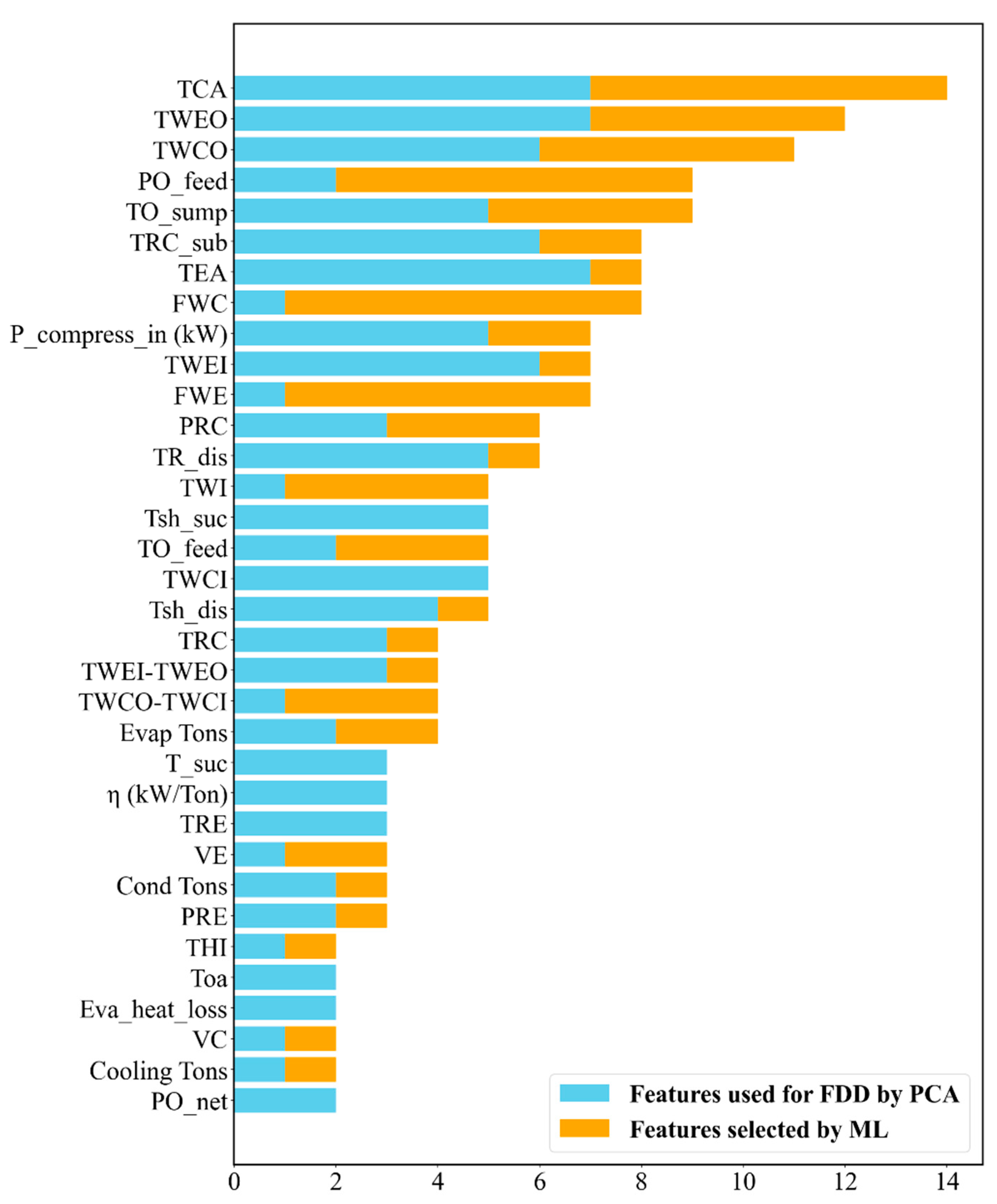
Figure 2 summarizes the most commonly used and selected variables presented in Table 1 and Table 2. This figure displays the frequency of each variable in descending order, highlighting how many times they were utilized by studies that used PCA for chiller FDD and were selected through machine learning models. Variables that were used or selected only once have been excluded from this figure. The Methodology (Section 3) and model implementation (Section 5) will discuss how the initial pool of variables is selected for this study.
An analysis of the selected variables and feature selection methods reveals that all approaches used for FDD have been supervised, while there are no studies specifically designed for identifying important variables in unsupervised techniques such as PCA. Furthermore, except for the work by Wang et al., most studies failed to consider the practical significance of variables, including the availability of sensors in the field, their thermodynamic relevance, and their role within the chiller loop. Another limitation of previous works is the assumption that all types of faults are known and available for model training and evaluation, while in practice, this scenario rarely occurs.
The highlights of the Literature Review Section can be summarized as follows:
  • Most existing filtering methods have focused on sensor fault detection and air handling units (AHUs), while the applicability of denoising techniques for detecting component-level faults in chillers has been far less explored.
  • While some studies have acknowledged the nonlinear behavior of chillers, the emphasis has primarily been on steady-state operation. The transient behavior, which introduces stronger nonlinearities, has largely been overlooked.
  • Although unsupervised techniques such as PCA have been widely used, the selection of sensitive and relevant variables to enhance their fault detection performance has received less attention. Most prior work has instead focused on identifying key variables for supervised fault detection and diagnosis.

3. Methodology

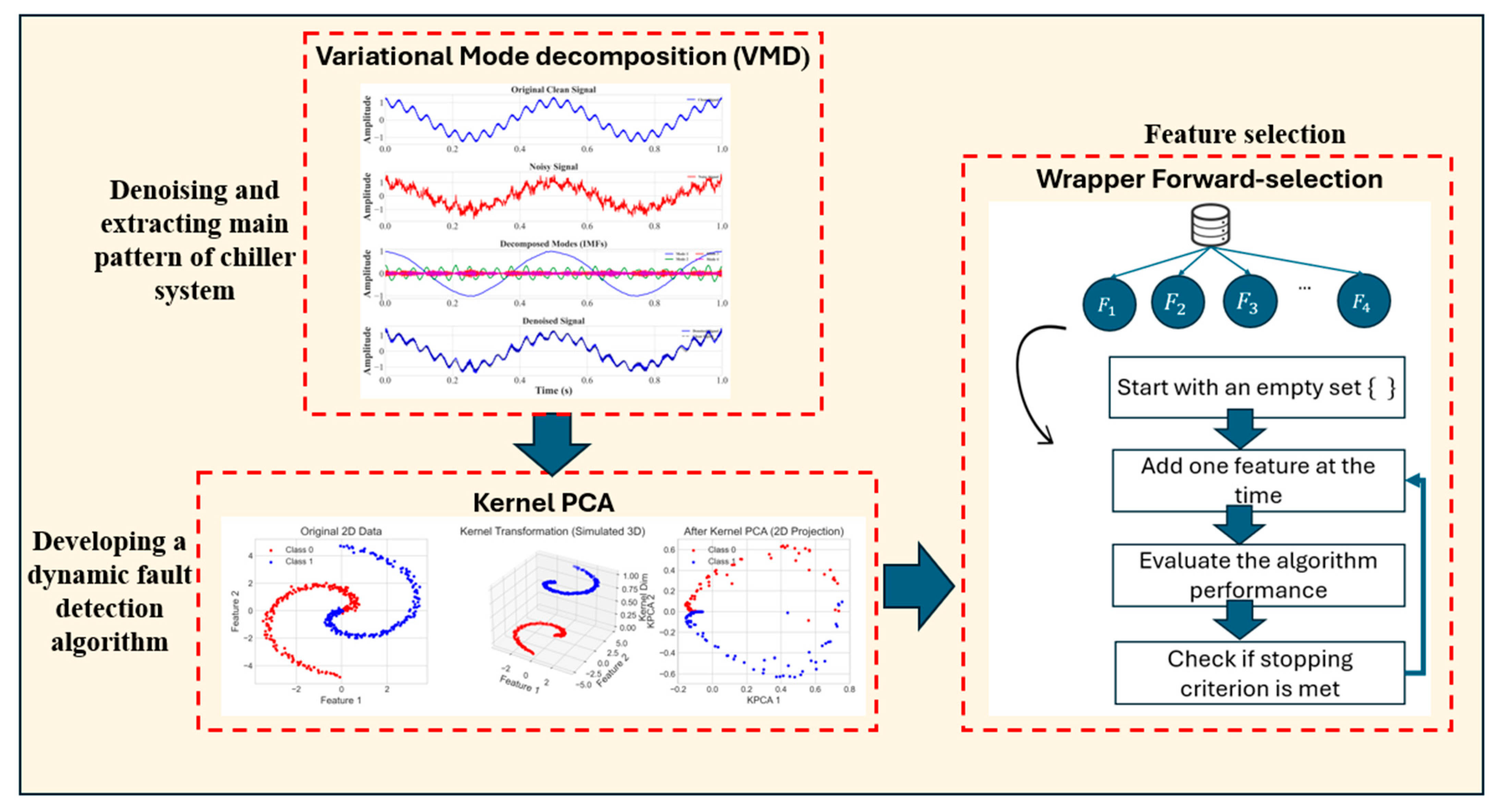
This section is organized into three subsections, as illustrated in Figure 3: the first covers the theory and formulation of the VMD method, the second outlines the foundation and formulation of KPCA, and the third section describes the feature selection framework.
The process begins by applying VMD to dynamic chiller sensor data. VMD decomposes each signal into intrinsic mode functions (IMFs), effectively removing high-frequency noise and fluctuations while extracting the dominant pattern of system behavior during the transient and steady-state conditions of the chiller. This improves the signal-to-noise ratio and makes the variables easier to analyze, enabling more effective feature selection and fault detection under dynamic conditions.
Next, to develop a robust fault detection algorithm, Kernel Principal Component Analysis (KPCA) is applied to the denoised, fault-free training data. KPCA models the system’s normal operating behavior by learning its nonlinear structure and underlying dynamics, making deviations easier to detect under dynamic operating conditions. Finally, a wrapper-based forward feature selection method is employed to identify the most informative subset of variables from a larger pool, ensuring that only the most relevant features are retained for accurate fault detection. The selected subsets maintain acceptable detection accuracy and false alarm rates even when certain sensors are missing, faulty, or not installed, allowing the method to remain robust under a reduced number of sensors.

3.1. Variational Mode Decomposition (VMD)

Chiller systems often operate under dynamic and noisy conditions, where sensor signals may be corrupted by fluctuations, electrical noise, or small disturbances unrelated to underlying system behavior. These irregularities can obscure the true structure of the data and negatively impact fault detection analysis. In this study, to remove noises and extract the main pattern of chiller behavior, VMD is employed as a preprocessing step for denoising chiller operational signals. By decomposing each raw signal into a set of modes and selectively reconstructing the signal using only the dominant modes, VMD allows us to remove high-frequency noise while retaining the main patterns of interest. The denoised signals preserve meaningful dynamics associated with normal and faulty operations that are more stable and reliable for FDD analysis. In the following, VMD formulation is discussed:
Variable Mode Decomposition (VMD) is a signal decomposition technique developed by Dragomiretskiy and Zosso to overcome the limitations of Empirical Mode Decomposition (EMD) [51] Unlike EMD, which extracts modes sequentially, VMD decomposes the signal into a set of band-limited intrinsic mode functions (IMFs) simultaneously, ensuring accurate reconstruction of the original signal. Therefore, the original signal f ( t ) is decomposed into finite k subseries or modes u k (k = 1, 2,…, K), each centered around a specific pulsation ω k , which is determined alongside the decomposition process. The decomposition is performed by minimizing the total bandwidth of all modes under the constraint that their sum reconstructs the original signal:
min u k , ω k t δ t + j π t u k ( t ) e j ω k t 2 2
s . t .             k u k ( t ) = f ( t )
To solve this constrained problem, an augmented Lagrangian formulation is introduced and optimized using the Alternating Direction Method of Multipliers (ADMM). The optimization proceeds iteratively by updating u k n + 1 , ω k n + 1 and λ k n + 1 . The resulting modes are compact, non-overlapping in frequency, and retain both the amplitude and frequency characteristics of the original signal.
Selecting the parameters of VMD, particularly the number of modes K into which a signal is decomposed, is a critical aspect of the method. Various approaches have been proposed in the literature to determine the appropriate mode number K , including entropy-based criteria, maximization of signal-to-noise metrics such as kurtosis, meta-heuristic optimization of VMD parameters, frequency or energy-based inspection of the decomposed modes for different candidate values of K , and sensitivity analysis through grid search to examine how different combinations of VMD parameters affect model performance and to identify the settings that maximize prediction accuracy [52].
In this study, our goal is to extract the main operational patterns of the chiller variables and suppress noise while maintaining high FDD accuracy and low computational cost. To achieve this, the signal is decomposed using several candidate values of K , and the energy distribution of the resulting modes is examined to determine whether increasing K meaningfully alters the energy of the dominant component. The normalized energy of the k -th mode is computed as [53].
E k = t u 2 ( t ) j = 1 K t u j 2 ( t )
where u k t is the k -th VMD mode. This metric represents the fraction of the total signal energy carried by the mode k . For each candidate K , the number of leading modes required to capture at least 95% of the original signal energy is determined. If the number of modes needed to reach the 95% threshold remains unchanged when K is increased, it indicates that additional modes do not contribute meaningful information. In such cases, the decomposition is considered saturated, and the smallest K that captures the dominant energy content of the signal is selected. This strategy allows us to identify both (i) the appropriate number of modes into which the signal should be decomposed and (ii) the subset of modes that should be retained for further analysis. By selecting the smallest K that preserves the dominant energy of the signals, the method balances information retention with computational efficiency, which is crucial for FDD and feature selection.

3.2. Kernel PCA

To address the nonlinear characteristics of the chiller system, the denoised signals obtained from VMD are used for developing Kernel PCA as a fault detection algorithm. Kernel PCA is a type of PCA developed by S c h o ¨ l k o p et al. to address the limitation of PCA, which uses a linear transformation to transform data to a lower-dimensional space. Instead, Kernel PCA maps data into a higher-dimensional feature space to handle nonlinear behavior before applying PCA calculations. The formulation and concept of Kernel PCA are presented below, while additional details and derivations are available in [54] for interested readers.
Assuming data matrix X =     x 1 ,   x 2 ,   ,   x n T   R n × m where x i R m is an m-dimensional column vector, n and m represent the number of observations (rows) and variables (columns), respectively. Data is mapped to a higher-dimensional space H using the mapping function Φ : x   R m   z   R h   to make data linearly separable. Instead of explicitly computing the mapping function Φ   ( x ) , the kernel trick provides a function equivalent to the dot product of the transformed data points Φ (   x i ) and Φ (   x j ) in the higher-dimensional space, and this can be represented as:
k x i , x j = φ i T φ j
Assuming that the training data in the feature space are represented as Φ = φ 1 φ 2 φ n T where each φ i R h is an h-dimensional column vector obtained by mapping the original data points into the high-dimensional feature space, and the covariance matrix ( C ^ R h × h ) is constructed in this feature space as follows:
n 1 C ^ = Φ T Φ = i = 1 n φ i . φ i T
The kernel matrix G is then defined using the kernel trick, where the kernel function k x i , x j can be polynomial, Gaussian, sigmoid, exponential, etc., represents the inner product in the feature space:
K = Φ Φ T = φ 1 T φ 1 φ 1 T φ n φ n T φ 1 φ n T φ n = k x 1 ,   x 1 k x 1 ,   x n k x n ,   x 1 k x n ,   x n
Principal components in the feature space are obtained by solving the eigenvalue problem:
β = K β
This reveals that β and are the eigenvector and eigenvalue of the kernel matrix K , respectively. The corresponding principal direction v i in the feature space is an h -dimensional column vector and is computed as:
v i = 1 i Φ T β i
The first principal eigenvectors corresponding to the largest eigenvalues in the feature space are then obtained as:
P f = v 1 v 2 v l = Φ T P Λ 1 / 2
where P = β 1 0 β l 0 and Λ = d i a g { 1 l } represent the l principal eigenvectors and eigenvalues of the kernel matrix.
The score of new measurement (x) in the feature space n the feature space is calculated using P f and its mapped vector φ as follows:
t = P f T φ = Φ T P Λ 1 / 2 T φ = Λ 1 / 2 P T Φ φ = Λ 1 2 P T k ( x )
where Φ ϕ is rewritten using kernel trick as
k x = Φ ϕ = ϕ 1   ϕ 2 ϕ n T ϕ = k ( x 1 , x )   k ( x n , x ) T
In this study, Kernel PCA is trained exclusively on fault-free data using selected key variables that represent both steady-state and transient operating behavior. By learning the nonlinear structure of these denoised signals, KPCA constructs a reference baseline that captures how the chiller naturally evolves during load changes, rather than assuming static operating conditions as in traditional PCA. During fault detection, new measurements, whether steady or transient, are projected onto this learned feature space, and deviation indices such as the Squared Prediction Error (SPE) or T2 statistics are computed. These deviation measures are compared with statistically derived thresholds to determine whether the system is operating normally or exhibiting fault-induced deviation from expected patterns.

3.3. Fault Detection

In this study, the Squared Prediction Error (SPE) defined as the squared norm of the residual vector in the feature space, is adopted. Specifically, the residual vector represents the component of the data that is not captured by the principal components and is associated with faulty conditions. Given that KPCA transforms the original data into a higher-dimensional feature space via a nonlinear mapping ϕ , the residual components in the feature space can be described by projecting the data onto the subspace orthogonal to the principal components. This projection is achieved using the residual loading matrix P ~ f , which is orthogonal to the principal components (PCs). Therefore, components in the residual subspace would be:
t ~ = P ~ f T φ
The Squared Prediction Error (SPE) is then calculated as the squared norm of these residuals:
S P E = t ~ T t ~ = φ       T P ~ f P ~ f T φ
To capture the faulty pattern, a control limit is required, and various thresholds for SPE have been proposed. In this study, we adopt the threshold originally developed by Box [55]:
S P E a = g χ h , a 2 ;               g = V 2 μ ,           h = 2 μ
where μ and V represent the mean and variance of SPE values corresponding to the normal operating conditions.

3.4. Feature Selection

In this study, both automatic and knowledge-based methods are used to select the most relevant variables for unsupervised fault detection. Initially, variables that govern the chiller system, commonly found in most systems and recommended by previous studies, are evaluated and selected. In the next step, the wrapper method—an iterative approach that selects subsets of features and evaluates a machine learning model’s performance to identify the most important features—is adopted and combined with the proposed VMD-KPCA method.
A wrapper method, which strategically evaluates the performance of a machine learning model using subsets of variables, is adopted and integrated with the VMD-KPCA method. Since the wrapper method is typically used with supervised machine learning algorithms, we assume that, in addition to fault-free data, only one type of faulty data is available. This assumption is more realistic compared to previous studies, which often assumed that all types of faults are available for training and evaluation. Although the KPCA model is trained solely using fault-free data, the wrapper-based feature selection procedure evaluates candidate subsets using limited labeled fault samples to balance MAR and FAR during feature ranking. This does not affect the unsupervised nature of the online detection stage.
In this study, the Forward Selection (FS) algorithm is employed to systematically identify the most informative features. This approach reduces the high computational cost associated with Kernel PCA when dealing with a large number of variables and has demonstrated strong performance in previous research [28] Unlike backward selection, which starts with all variables and increases complexity, FS incrementally builds the model, reducing runtime and avoiding redundant inputs.
The FS method initiates with an empty set, systematically adding one attribute at a time to evaluate model performance. The FS method initiates with an empty set, systematically adding one attribute at a time to evaluate model performance. In a scenario with m variables, the model is trained and evaluated m times during the first step, with each iteration adding one different variable to the feature set. The model’s performance is compared across these iterations, and the variable that results in the best performance is selected. In the second round, with the first feature selected, the remaining m 1 variables are each added to the selected feature, and the model is trained and evaluated m 1 times over pairs of variables. This process continues for subsets of 3, 4, and so on, until the convergence criterion is met, which could be a specific accuracy threshold or when the performance plateaus.
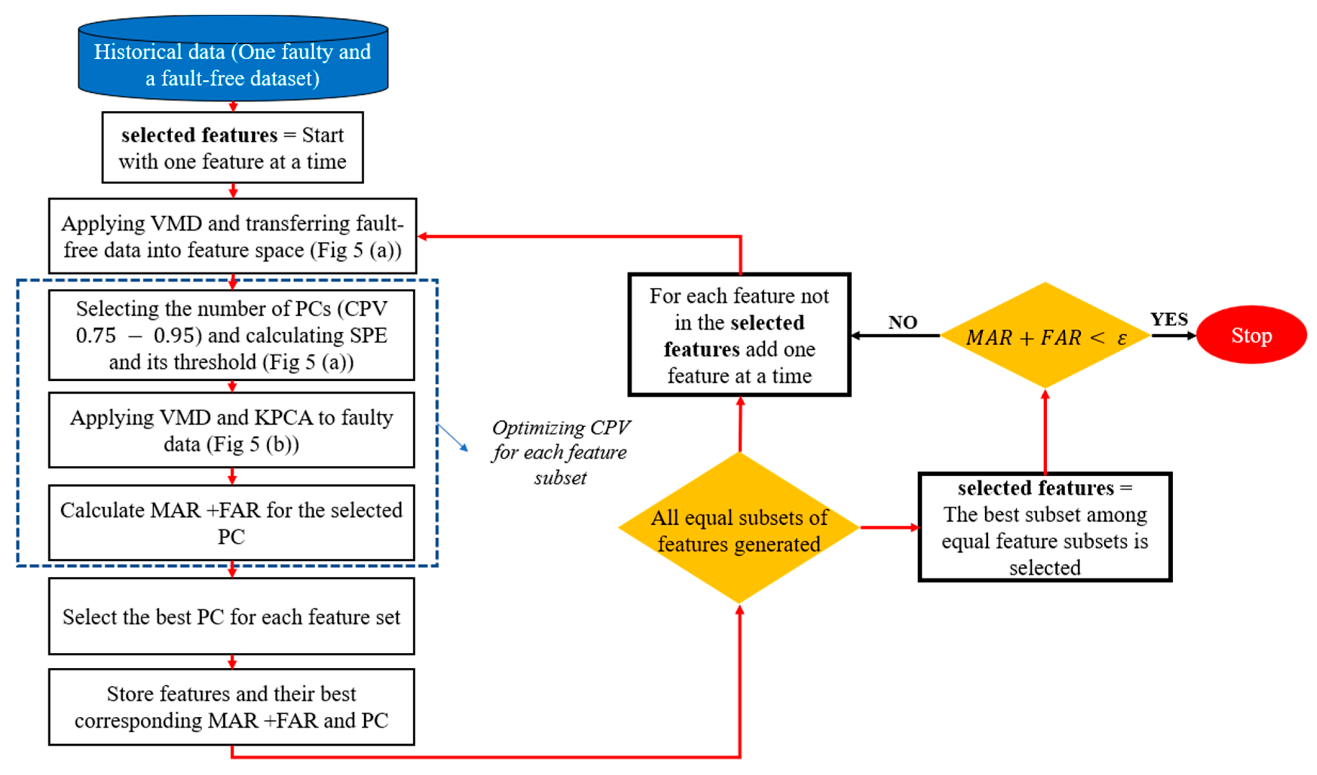
For each subset, VMD is applied to both fault-free and faulty datasets. The data are then transformed into a higher-dimensional space using Kernel PCA to minimize the Missing Alarm Rate (MAR) and False Alarm Rate (FAR) for effective fault detection. Optimizing KPCA parameters is essential for identifying the features that best reduce MAR and FAR. One key parameter is the cumulative percentage of variance (CPV), which represents the data variance captured by the principal components. In HVAC system studies, CPV thresholds typically range between 75% and 95% [36]. Here, CPV is optimized to minimize the combined sum of MAR and FAR.
CPV can be selected and tested by trial and error or optimization algorithms such as Particle Swarm Optimization (PSO). Therefore, a different value for CPV between 0.75 and 0.95 is generated, and the performance of VMD-KPCA is evaluated using the calculation of MAR and FAR.

4. Case Study

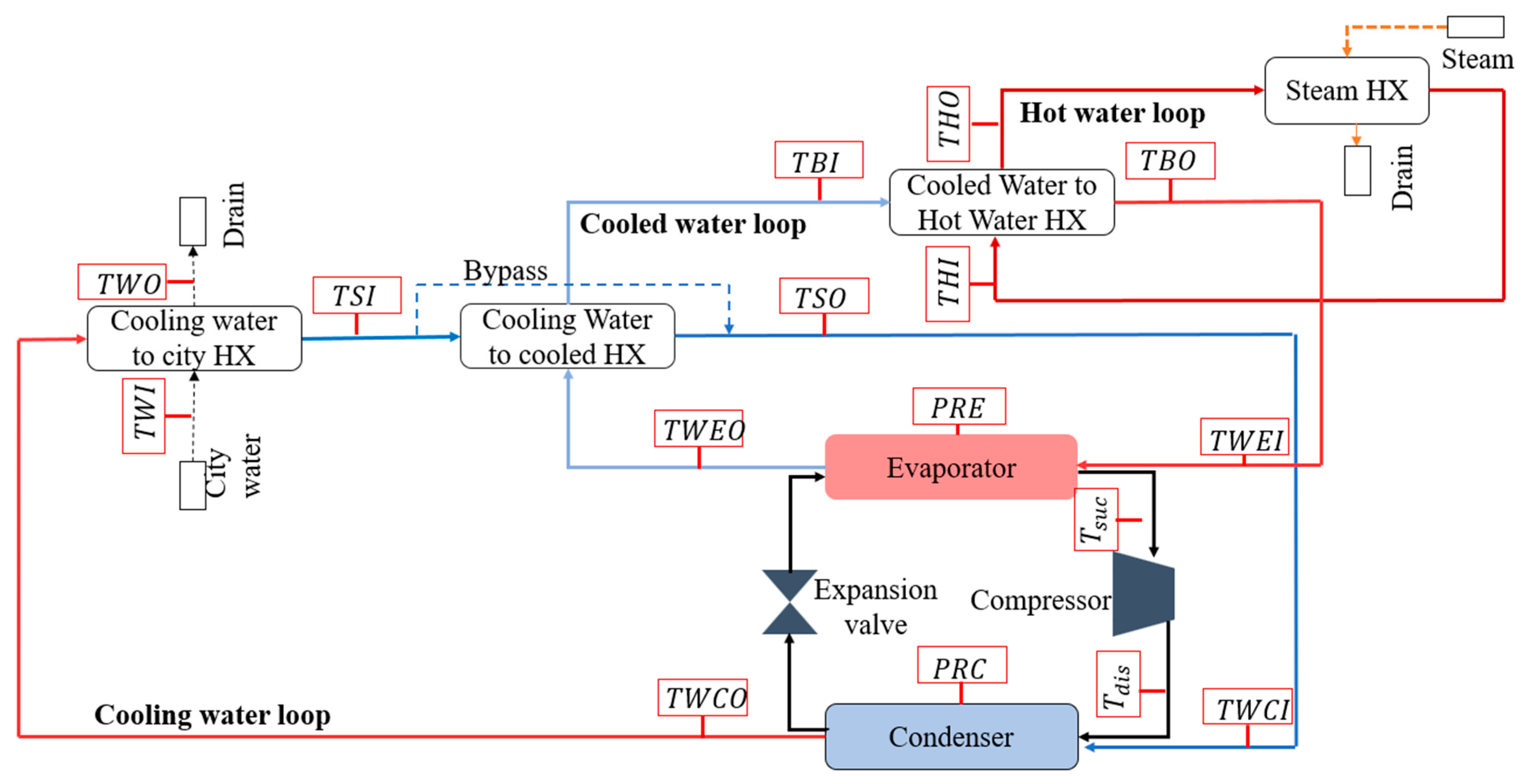
In this study, the ASHRAE RP-1043 dataset, which is a 90-ton water-cooled chiller consisting of a shell-and-tube evaporator, a shell-and-tube condenser, a pilot-driven expansion valve, and a centrifugal compressor, as depicted in Figure 4, is used to validate the proposed method. In addition to the refrigeration cycle, the chiller facility has five water circuits, including the evaporator water circuit, condenser water circuits, hot water circuit, city water supply, and steam supply. The chiller system was tested under fault-free conditions as well as with seven distinct fault types introduced at four severity levels: condenser fouling (CF), non-condensable gas (NCG) presence, reduced condenser water flow rate (RCW), reduced evaporator water flow rate (REW), refrigerant leakage (RL), refrigerant overcharge (Refover), and Excess oil (Exoil). In total, 64 variables were monitored, consisting of 48 directly measured variables and 16 calculated ones, under both normal and faulty conditions. To consider all potential operational scenarios encountered by the chiller, three key parameters—cooling load, temperature of water entering the condenser (TWCI), and temperature of water entering the evaporator (TWEO)—were varied at three different levels, resulting in data across twenty-seven distinct operational conditions. The test took slightly more than 14 h, and a total of 5191 samples were recorded at 10 s intervals, allowing for the capture of both steady and transient behaviors, including start-up, shutdown, and shifts caused by changes in any of the three operational parameters.

5. Model Implementation

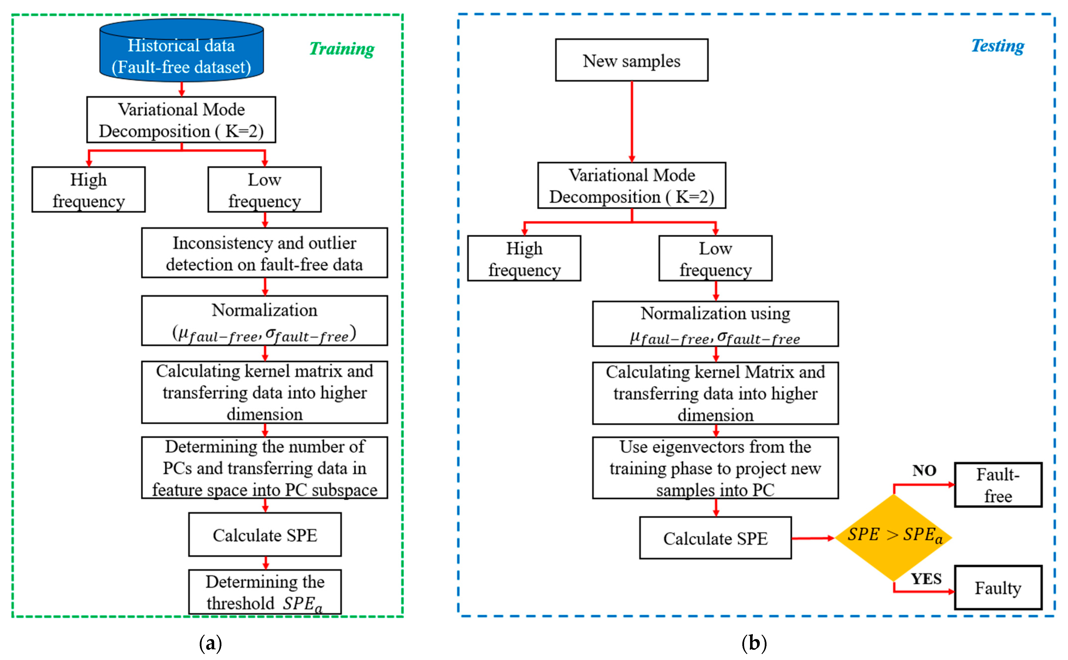
This section outlines the step-by-step application of the proposed methodology to the chiller dataset. Figure 5 illustrates the integration of VMD and KPCA during the training and testing phases.
The first step involves decomposing the data and selecting VMD parameters. In this study, the number of VMD modes was set to K = 2 to separate the data into a dominant low-frequency component and a higher-frequency fluctuation component. Before fixing this value, a preliminary test with K = 1 , , 8 and evaluated the cumulative energy distribution of the resulting modes. The results showed that increasing K beyond 2 did not meaningfully change the energy captured by the primary mode, while the additional modes mainly represented low-energy, noise-like components. Considering that the subsequent steps (KPCA and feature selection) are computationally expensive, choosing the smallest K that preserves the dominant dynamics reduces computational complexity without affecting detection performance. Higher K may be beneficial in applications where high-frequency resonance modes carry significant fault information, but the results indicate it is unnecessary for the chiller faults considered here.
To ensure there are no outliers or inconsistencies, the interquartile range (IQR) method is applied to the low-frequency data. By calculating the first and third quartiles, we establish the upper and lower bounds of the data, and any data points outside this range are identified as outliers. This outlier detection is not applied in the testing phase, as outliers may provide valuable insights into faulty patterns within the data.
Before applying KPCA, the data is normalized using z-score normalization. A second-order polynomial kernel is utilized to map the data into a higher-dimensional space due to its simplicity as one of the least complex nonlinear kernels, being computationally less expensive, and requiring minimal hyperparameter tuning [54].
k x i ,   x j = x i T x j + c d
To transform data into the feature space to the principal component (PC) subspace, the number of PCs is selected to capture 95% of the variance for the reference case. The reconstructed error, or SPE, for the fault-free data and the corresponding threshold are calculated using Equations (13) and (14), respectively. In the testing phase, low-frequency data is normalized using the parameters obtained from the fault-free training data, and the feature space data is projected into the PC subspace using eigenvectors derived from the system’s normal behavior. The SPE of new samples is then calculated and compared against the threshold. Samples with SPE values exceeding the threshold are classified as faulty; otherwise, they are considered fault-free.
In this study, the VMD-KPCA method is applied to detect a fault at severity level one, the most challenging level to identify. Out of the 64 available variables, 33 variables, listed in Table 3 and referred to as Case 1, were selected as the initial feature pool based on the variables that were frequently used and selected in the literature (as shown in Figure 2) and their thermodynamic relevance to chiller operation and their thermodynamic significance. A careful review of the variables in Figure 2 reveals that certain features, such as TWI and THI, were specifically designed and recorded for the ASHRAE experiment and are not typically found in field data. In contrast, other critical features, like COP, were not commonly selected in prior studies, while it is one of the primary parameters in a chiller system that indicates system performance and thermodynamic behavior. Additionally, variables such as lift pressure, which represents the difference between condenser and evaporator pressures and reflects the compressor work required, were not selected, although they help explain reductions in subcooling. Another variable included in the analysis is the chiller heat balance, defined as the total energy input—comprising the heat absorbed by the evaporator and the compressor power—minus the energy rejected by the condenser. This parameter serves as an indicator of the system’s overall performance.
In practice, not all 33 sensors may be installed or calculated in field applications. To address this limitation, an alternative variable pool is considered for feature selection to identify a subset of variables. In this second case, parameters related to the lubrication system, such as T O s u m p , and flow parameters that are not typically measured are excluded from the initial pool. The focus shifts to parameters related to the vapor compression cycle to evaluate whether the model can detect faults without measurements from certain parts of the chiller system. Accordingly, only sensors commonly installed in the field, as suggested by Wang et al. [48], and variables derivable from those sensors are included in the initial pool. The proposed feature selection algorithm, illustrated in Figure 6, is then applied to both cases to identify the most critical features for dynamic fault detection.
The algorithm begins with an empty feature set. In the first round, each feature is individually added to this set, and VMD is applied to the dataset as illustrated in Figure 6. A critical step in the process involves selecting the optimal number of principal components (PCs) to retain. According to the literature, PCs should capture between 75% and 95% of the cumulative data variance. Consequently, the number of eigenvectors used to map the data into the PC subspace is determined by optimizing cumulative percentage variance (CPV) to minimize the sum of the MAR and FAR. As outlined in the methodology, the feature selection method assumes the availability of at least one faulty dataset. For this case, refrigerant leakage, which is one of the most challenging faults to detect in the early stages, was assumed to be available. In each iteration, after selecting the number of PCs, fault-free and refrigerant leakage data are mapped into the PC subspace, where SPE values are calculated and compared against a threshold defined by normal behavior to compute MAR and FAR. This process is repeated until the optimal number of PCs is determined, either through trial and error or with optimization algorithms such as Particle Swarm Optimization (PSO). After all equal-sized subsets of variables are created, their respective Missing Alarm Rate (MAR) and False Alarm Rate (FAR) sums are compared, and the subset with the lowest MAR + FAR is selected. If the MAR + FAR for the chosen feature subset is below a predefined threshold, the algorithm terminates. the algorithm continues adding new variables to the selected feature set from the previous round (e.g., when ε = 10%, corresponding to a 5% false alarm rate at a 95% confidence level and an acceptable MAR of 10–15% as reported in the literature).

6. Results and Discussion

This section presents and analyzes the outcomes of the proposed methodology, focusing on dynamic fault detection by VMD-KPCA, as well as the selection and influence of specific variables on detection performance. Squared Prediction Error (SPE) values, summation of Missing Alarm and False Alarm Rate (MAR and FAR), and Fault Detection Accuracy (FDA) are presented to evaluate the performance of the proposed FD framework.
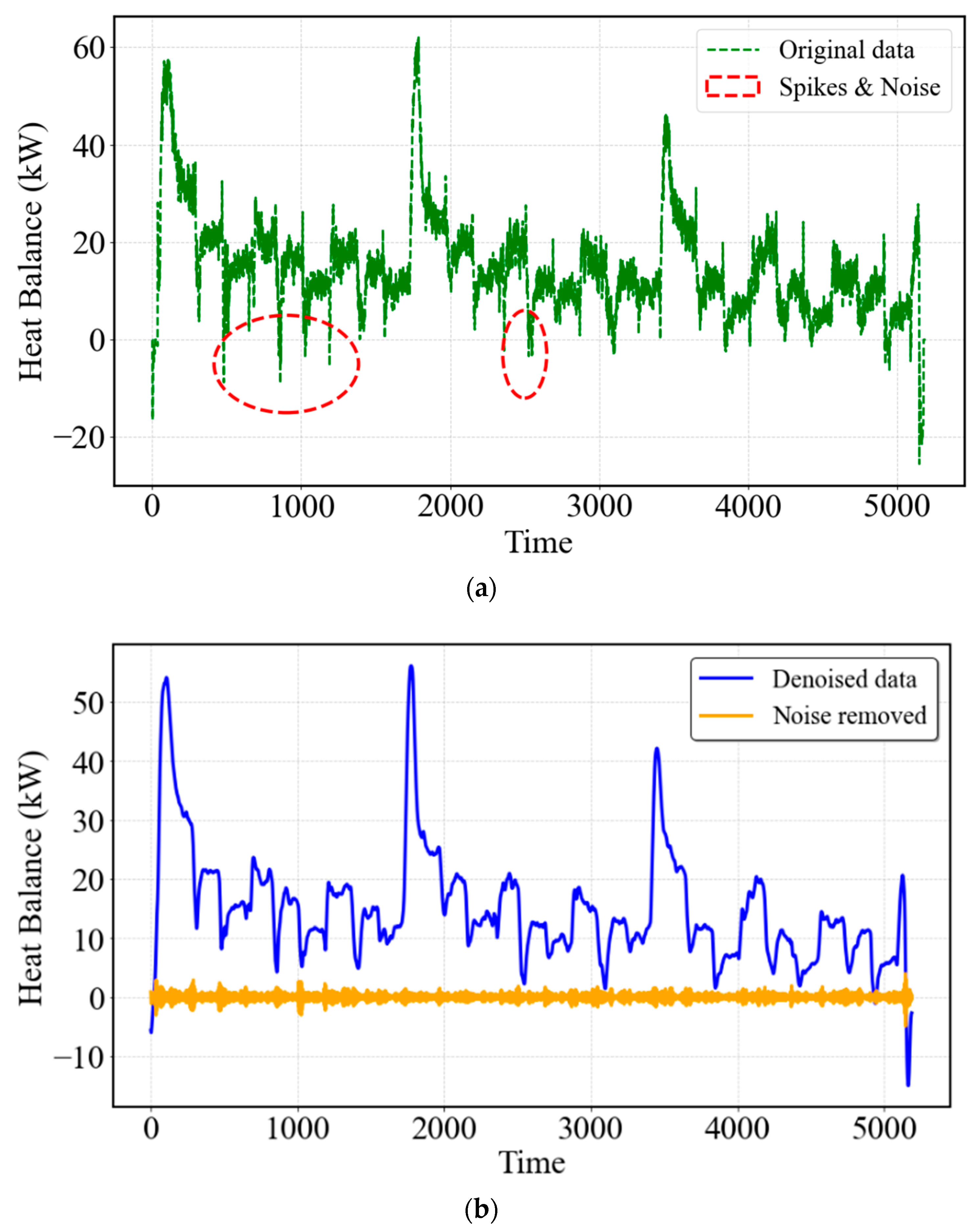
The initial step in the proposed fault detection framework involves decomposing the data into high- and low-frequency components to enhance data quality and interpretability. Figure 7a illustrates the original heat balance signal across various operational conditions, where large fluctuations and abrupt spikes, including both positive and negative deviations indicated by red circles, are evident. The regions highlighted with red circles may not accurately reflect the system’s physical behavior and are likely caused by measurement noise, sensor drift, or transient disturbances. By applying VMD, the resulting denoised signal (blue) exhibits a smoother trend, while the high-frequency components associated with noise (orange) are isolated and removed, as shown in the denoised graph in Figure 7b.
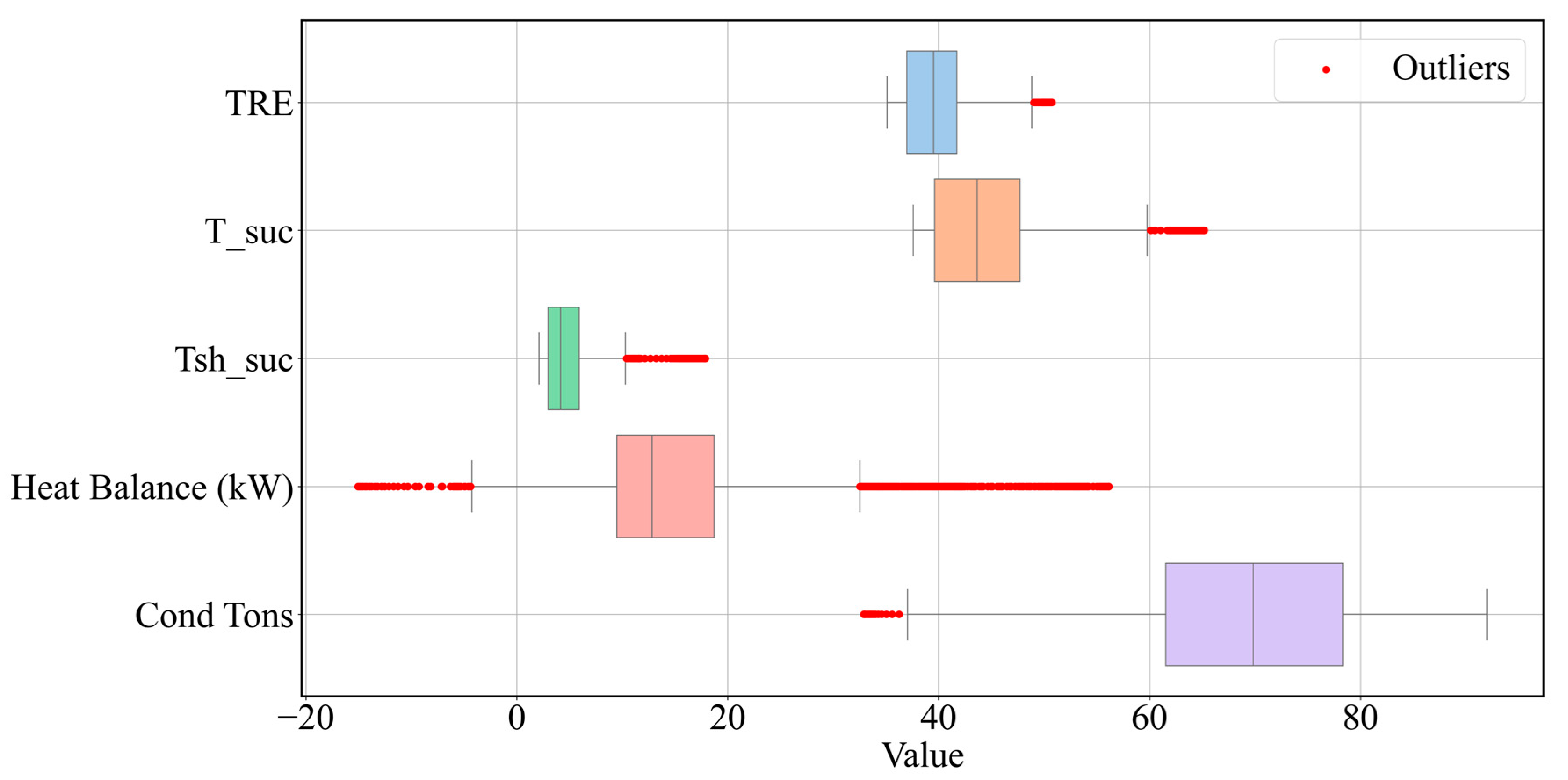
To ensure data consistency and eliminate outliers, the Interquartile Range (IQR) method was applied to each variable. The range of some variables, including evaporator temperature (TRE), suction temperature ( T s u c ), heat balance, and condenser ton out of range, is presented as a box plot in Figure 8. The plot reveals that some data points deviate significantly from the main range, indicating the presence of outliers. Further analysis shows that these outliers are associated with the system’s start-up and shutdown transients. Although these transient modes can offer valuable insights for fault detection, they may diminish the effectiveness of PCA models when combined with data from other transient conditions due to operational changes, as well as steady-state data. The start-up and shutdown phases exhibit sharp changes and a broad range of values, giving them unique characteristics distinct from other operational states. Therefore, it is recommended to analyze start-up and shutdown behaviors separately and to consider training the PCA and KPCA models specifically for these modes. This approach enhances fault detection accuracy by reducing potential confusion in the model, thereby improving its reliability across varying conditions.
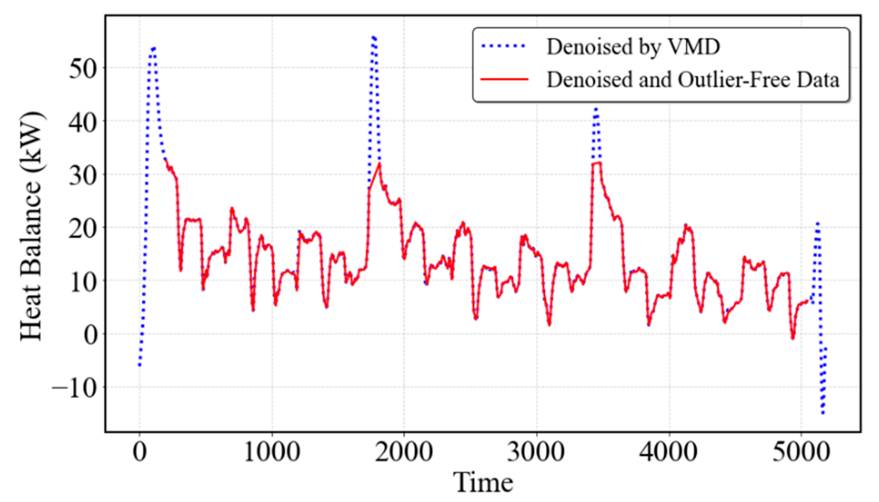
Figure 9 shows the heat balance data after removing start-up and shutdown values, along with any remaining outliers present across variables in the dataset. The IQR method is applied to each variable, and whenever an outlier is detected in any variable, the entire sample (i.e., the full set of variable values for that instance) is excluded. This approach ensures that no null values are introduced, thereby maintaining the consistency and integrity of the dataset for subsequent analysis.
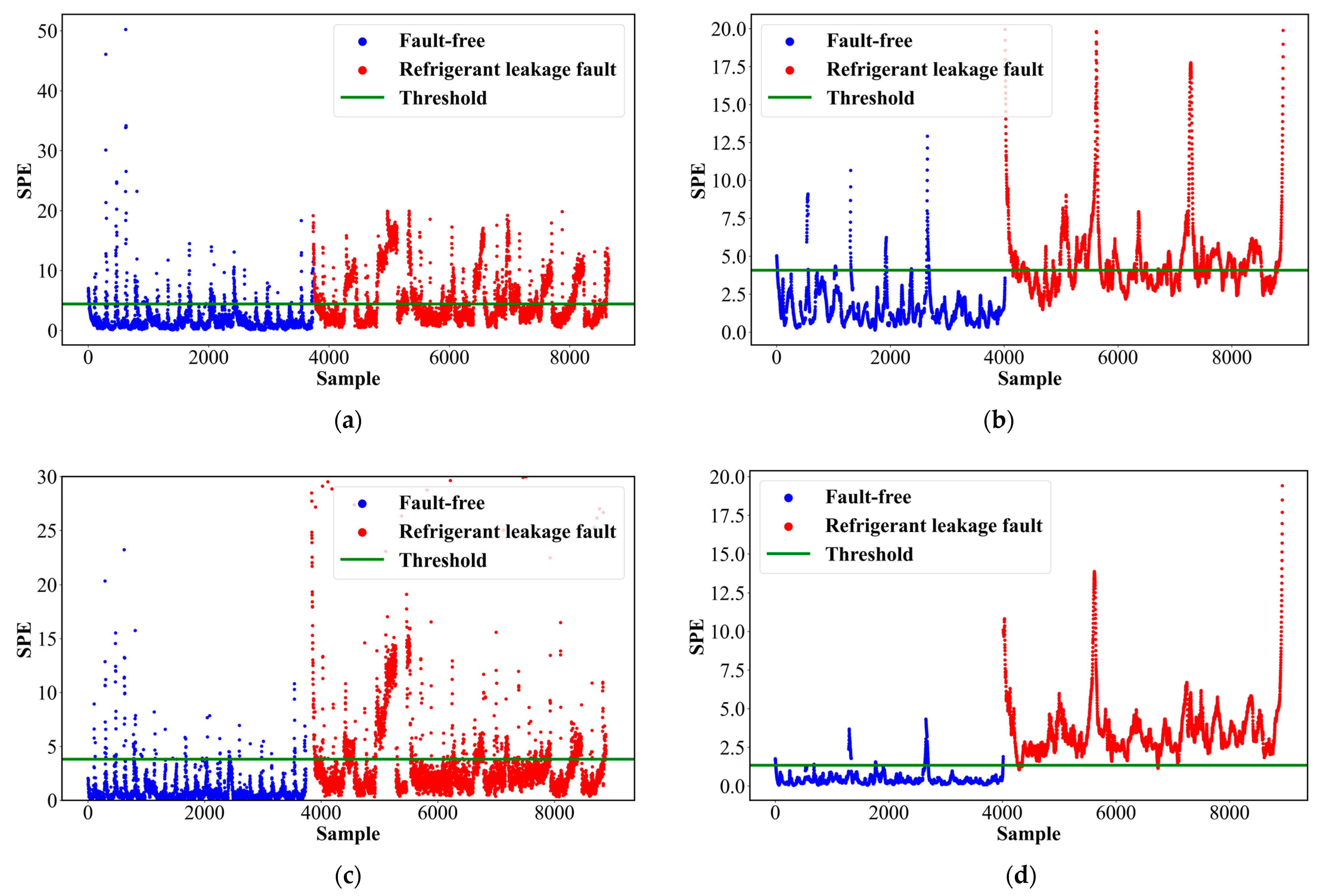
After outlier removal, 4015 data points across the 33 variables as the initial and reference cases remain, which are then normalized and prepared for training the KPCA model. In Figure 10, traditional PCA and KPCA models are compared both before and after applying VMD, based on the SPE values of fault-free and refrigerant leakage fault data indicated by blue and red dots, respectively. As shown in Figure 10a,c, both linear PCA and KPCA struggle to effectively detect faults without denoising the data, while outliers were removed from the fault-free data before training PCA and KPCA. These results show the impact of noise and other inconsistencies in the raw data, which obscure the fault patterns. Figure 10b,d illustrate that when VMD is applied, the separation between fault-free and faulty data becomes more distinct, as VMD helps filter out high-frequency noise and irrelevant variations in the data. Therefore, both linear PCA and KPCA fault detection accuracy significantly improve, particularly for KPCA, where a 98% FDA is achieved, indicating that it can accurately distinguish faulty samples from normal operating conditions. In contrast, although the VMD-based denoising step improved the performance of linear PCA, increasing its accuracy to 55%, this result confirms that PCA’s linear structure still limits its ability to capture the complex fault patterns present in the data.
These results underline the key contributions and effectiveness of the proposed hybrid method.
First, it is demonstrated that combining denoising, filtering outliers, and isolating start-up and shutdown transients for separate analysis can substantially enhance the fault detection performance of both PCA and KPCA. Moreover, employing nonlinear approaches such as KPCA rather than relying on the traditional PCA method effectively captures the chiller system’s nonlinear and dynamic behaviors and improves fault detection accuracy significantly. In other words, given the clear separation between the SPE values of fault-free and faulty conditions, dynamic fault detection becomes feasible when appropriate preprocessing is applied to the chiller system.
However, these results assume the availability of 33 sensors and variables, which is rather unrealistic for real-world characterization of the faults. Furthermore, some sensors in the field may encounter issues like calibration errors or faults, potentially limiting fault detection accuracy. Therefore, selecting a subset of variables that can effectively detect faults and optimize fault detection and diagnosis (FDD) performance is essential for these cases. Furthermore, reducing the number of variables can decrease computational complexity, which is especially important for KPCA, as it is more computationally intensive than linear PCA.
The next section discusses the two alternative pathways for the selection of features from the pool of variables. The feature selection process ensures the robustness and computational efficiency of the fault detection algorithm, subject to the varied availability of the variables.

6.1. Case 1—Variables Used and Selected in the Literature

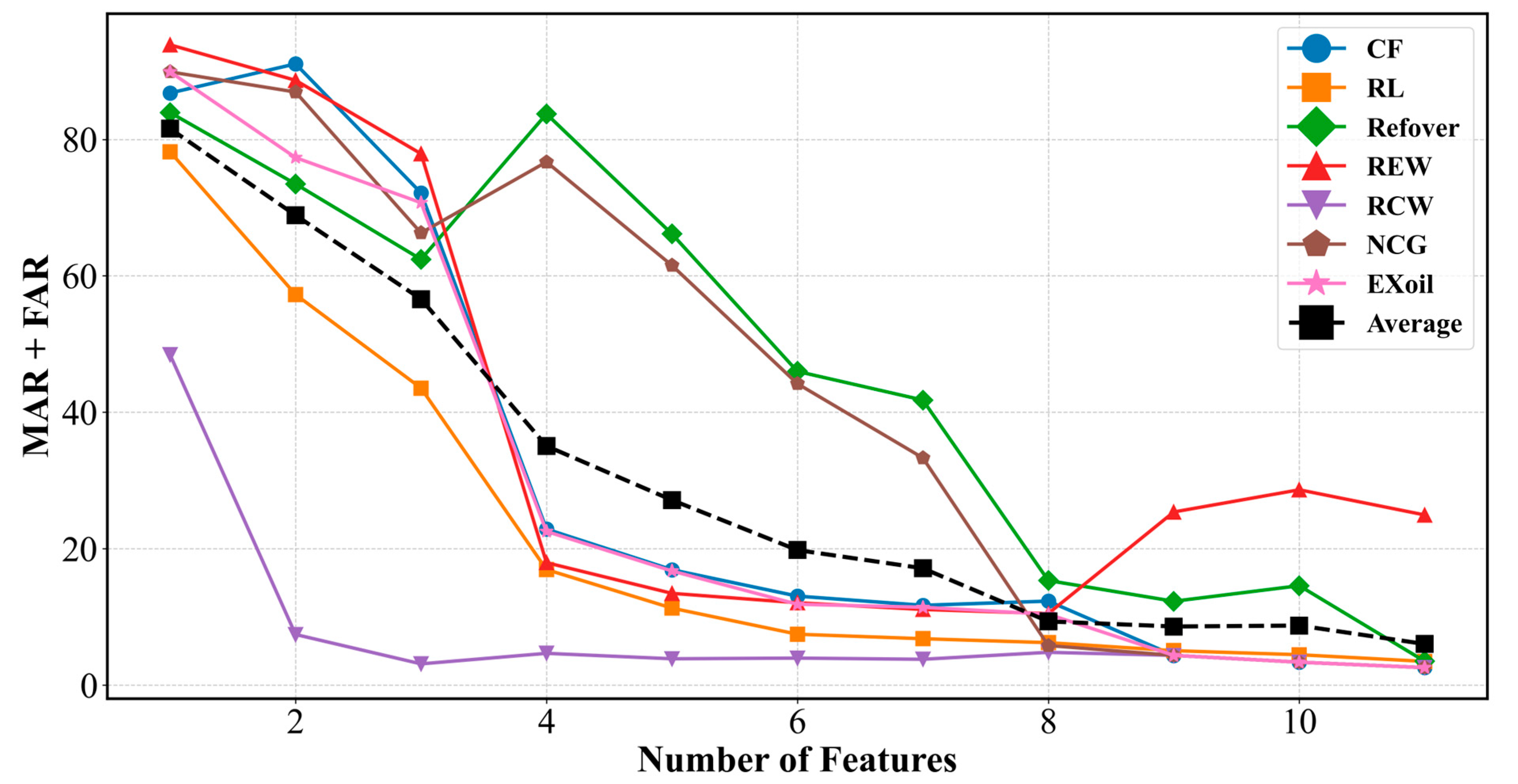
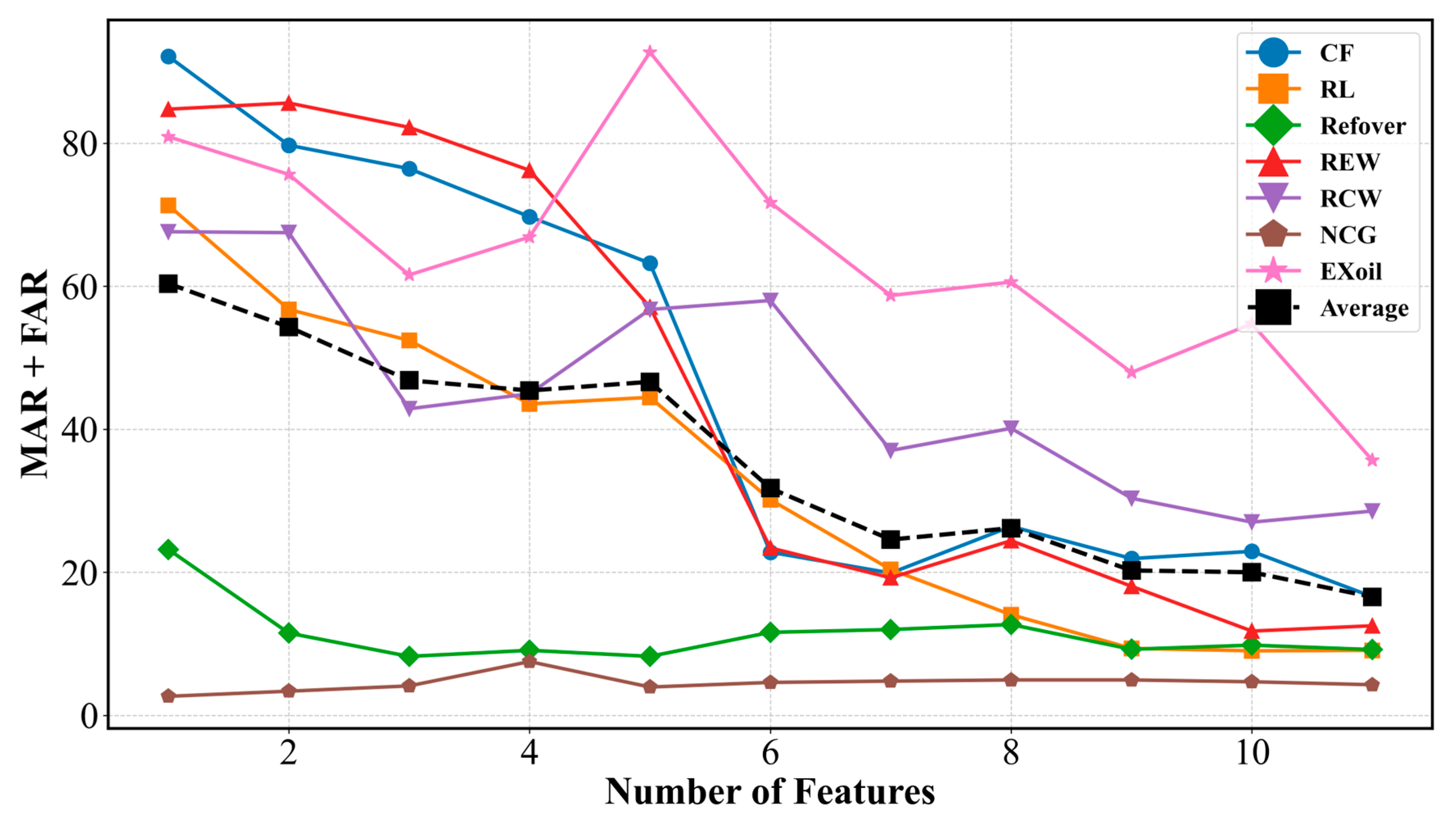
Using the proposed feature selection framework, subsets of features that are selected sequentially are reported in Table 4, along with the fault detection accuracy for seven types of faults. As previously discussed, the model is trained under the assumption that refrigerant leakage fault data is available. Therefore, VMD-KPCA prioritizes features that are highly sensitive to refrigerant leakage, capturing variables that exhibit significant deviations and account for the maximum variance in the data. After the variables are selected, the model is tested on six other types of faults to evaluate whether the chosen variables can effectively detect these faults as well. The proposed model selects variables that minimize MAR + FAR, as illustrated in Figure 11. This figure highlights the results for refrigerant leakage, the six other faults, and the average MAR + FAR across all fault types.
The average summation of the missing alarm rate (MAR) and false alarm rate (FAR) shows a continuous decreasing trend as the number of selected variables increases. A similar trend is observed for the average fault detection accuracy (FDA), except for two instances: when the number of variables increases from one to two and from nine to ten. The higher average FDA when only one variable is used compared to two variables can be attributed to an initial over-detection of faults. At the start, both fault-free and faulty samples are classified as faulty, leading to a seemingly high FDA, but this comes at the cost of a high false alarm rate, explaining the high MAR + FAR at the beginning.
According to Table 4 and Figure 11, although adding more features improved FDA and reduced MAR + FAR, it is noteworthy that an FDA greater than 90% and MAR below 5% can be achieved with only eight features. While increasing the number of features to 11 slightly raises the average FDA, it does not necessarily enhance the detection accuracy for all fault types. For instance, in the case of reduced evaporator water flow rate (REW), the FDA decreases when the number of features exceeds eight. This decline may be due to the inclusion of irrelevant variables such as P O n e t and T O s u m p , which exhibit minimal deviation from normal chiller behavior in the ASHRAE report. Including such features can confuse the model and degrade its ability to accurately detect the REW fault.
The following section provides a detailed discussion on the impact of various faults on the system, emphasizing the importance of selecting appropriate variables and their role in enhancing the fault detection accuracy of the model.
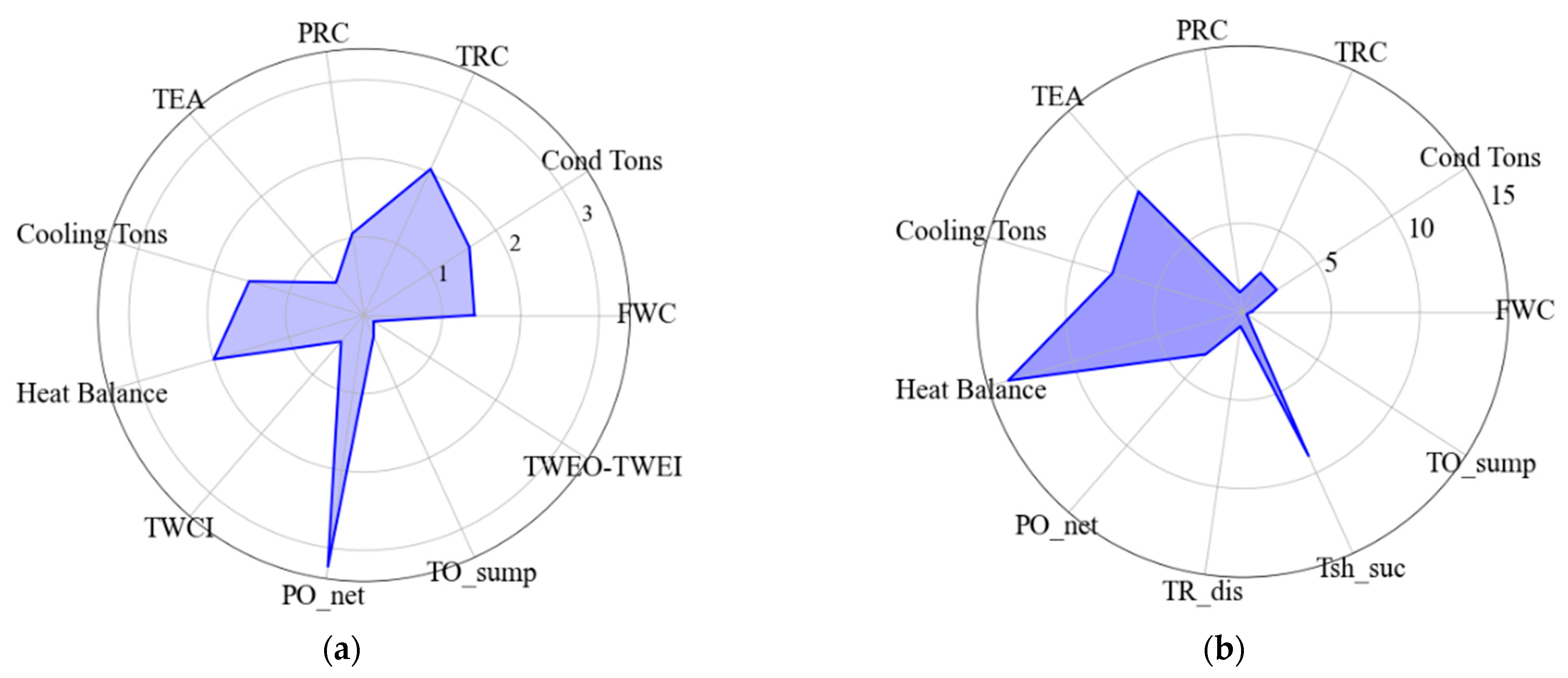
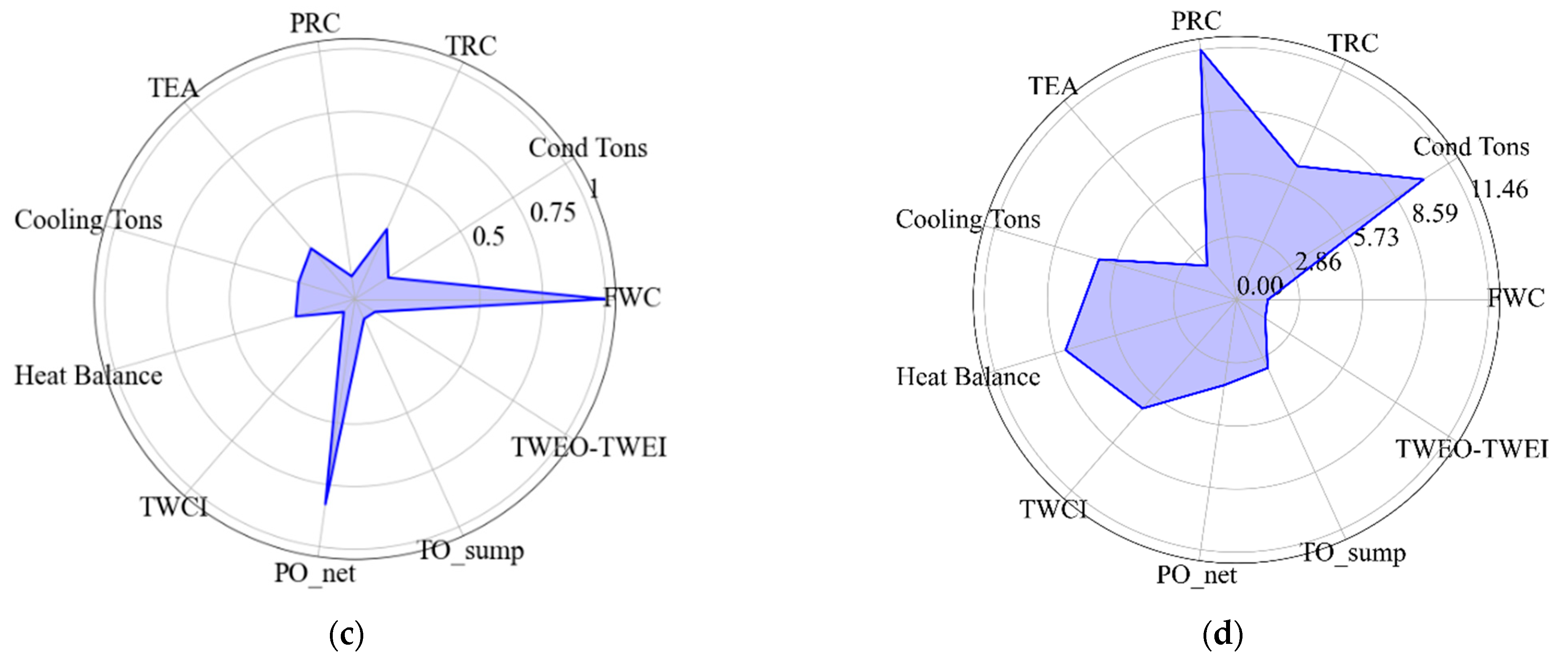
To simulate a refrigerant leakage fault, the total refrigerant charge of 300 lb is reduced incrementally by 10% for each severity level. A reduction in refrigerant charge leads to lower pressure in both the condenser and evaporator (PRC and PRE), as well as changes in associated saturated temperatures (TRC and TRE). According to the ASHRAE report, while these effects are relatively minor at the first severity level, they become more pronounced with increasing severity. Selecting condenser pressure and temperature (PRC and TRC) has significantly enhanced the fault detection accuracy of the VMD-KPCA model by raising the FDA to 87%. Furthermore, it is important to emphasize that KPCA accounts for the combined effect of variables and identifies the directions in the data that maximize variance. Another parameter affected during the test was the approach evaporator temperature (TEA) and P O n e t , whose selection by VMD-KPCA further contributed to the FDA improvement. One of the surprising variables selected for detecting refrigerant leakage was the Condenser Water Flow Rate (FWC), which is not typically expected to change in response to a refrigerant leakage fault since it is not controlled within the system’s control loop. Under normal conditions, FWC was set to 270 gpm, and it was only changed during testing to simulate a reduced condenser water flow rate. To investigate why FWC was selected as the first variable for detecting Refrigerant Leakage (RL), the average error between fault-free and faulty data, the average percentage error to capture relative deviations, and the average error for scaled data to assess the impact of normalization were calculated and are plotted in Figure 12. The analysis reveals that variables such as P O n e t , TRC, Heat Balance, and FWC exhibit higher deviations from fault-free conditions, as shown in Figure 12a. Specifically, the average deviation of FWC from its normal condition is 1.4 gpm, which is smaller than the measurement uncertainty of ±2.2 gpm, and this corresponds to a percentage error of 0.5% as illustrated in Figure 12b. This suggests that the observed deviation may result from measurement errors or system fluctuations rather than actual fault-related changes. However, prior to applying KPCA, the data are normalized. While normalization ensures that variables are scaled comparably, it can also inadvertently amplify small, non-critical differences, making them appear more significant. This effect is evident in Figure 12c, where the normalized deviation of FWC from the fault-free condition is greater than that of all other variables, explaining why FWC was selected as the first variable for detecting RL. This phenomenon can be attributed to a characteristic of z-score normalization, where variables with low standard deviation result in larger z-scores for small deviations from the mean. As shown in Figure 12d, the standard deviation of FWC is notably lower compared to other variables. Because the standard deviation appears in the denominator of the z-score formula, this low variability amplifies the normalized deviation of FWC from the fault-free condition. In addition, this is combined with sensor uncertainty and denoising, causing small measurement differences between fault-free and refrigerant leakage conditions to appear larger after normalization. This amplification leads to an exaggerated distinction in the normalized data, making FWC appear more sensitive to faults in KPCA-based detection despite the actual physical change. This observation underscores the importance of thoroughly understanding the system’s behavior, as well as the limitations and potential pitfalls of statistical and machine learning methods. Such understanding is crucial to avoid misinterpreting results and applying these methods blindly, which could lead to inaccurate conclusions or suboptimal fault detection.
Unlike refrigerant leakage, Refrigerant Overcharge (Refover) was simulated by adding excess refrigerant to the system. According to the ASHRAE report, subcooling temperature and condenser approach temperature are significantly affected by this fault, yet they were not selected as variables for fault detection. Instead, condenser temperature and evaporator approach temperature demonstrated deviations from normal system behavior, making them effective for detecting Refover. Furthermore, incorporating cooling tons and heat balance as features enabled KPCA to better capture the patterns of normal data and more effectively highlight the deviations caused by Refover.
Although FWC is not directly affected by the refrigerant leakage fault, it, along with the condenser valve position, plays a key role in detecting reduced condenser water flow (RCW) since the condenser flow rate was intentionally reduced to simulate this fault. As observed in Figure 11, RCW fault exhibits the lowest MAR + FAR among all other faults, and all faulty samples are correctly identified as faults using only FWC. However, MAR + FAR is high initially due to a high false alarm rate in the early steps. As the number of features increases and the model captures the pattern of fault-free data more accurately, the false alarm rate decreases.
Similar to the RCW fault, the reduced evaporator water flow (REW) fault is simulated by decreasing the evaporator water flow rate through adjustments in the evaporator valve position. However, these two variables were not selected during feature selection because they remained constant under refrigerant leakage fault conditions. The selection of TEA and Heat Balance, which reflect evaporator behavior, improved the fault detection accuracy (FDA) for REW faults. Conversely, selecting lubrication-related parameters such as P O f e e d and oil temperature in the sump ( T O s u m p ) resulted in a decrease in the FDA. This aligns with the findings in the ASHRAE RP-1043 report, where these parameters exhibited very minor deviations from their normal values, indicating that they are not useful for detecting REW faults. Furthermore, their inclusion alongside the list of variables selected appeared to dilute the KPCA’s ability to distinguish REW faults effectively. The parameter significantly impacted by the REW fault is the difference between the evaporator inlet and outlet water temperature (TWEI-TWEO), which is also highlighted in the report. Including this parameter enhanced the FDA for REW faults to some extent, although it could not restore the FDA to the levels observed before the oil-related parameters were selected.
In the ASHRAE experiment, condenser fouling was simulated by partially blocking condenser tubes. This fault affects the condenser water flow rate; however, the report indicates that even a 45% reduction in tube area only decreases the flow rate by 5%. This explains why selecting FWC did not significantly improve fault detection accuracy for CF at the first severity level, where only 12% of the tubes are blocked. The reduction in condenser surface area decreases the effective heat transfer coefficient, leading to lower saturation temperature and pressure. As a result, selecting TRC and PRC significantly improves CF fault detection accuracy, increasing FDA from 16.3% to 81.7% while also reducing missing alarm and false alarm rates. The inclusion of evaporator approach temperature (TEA) further enhances FDA, as TEA shows substantial deviation from fault-free conditions, particularly at the first severity level. However, at higher severity levels, the deviation in evaporator approach temperature diminishes due to the expansion valve’s response to superheat temperature changes.
Excess oil faults occur due to an excessive amount of oil in the system, often introduced during servicing or maintenance. Detecting this fault is facilitated by monitoring oil-related parameters, such as pressure and temperature. This is evident from the selection of P O n e t , a parameter that demonstrated significant deviation and clear interpretability for this fault, contributing to an improved Fault Detection Accuracy (FDA) of 100%. Excess oil impacts compressor performance, as observed through increasing deviations in compressor-related variables with higher fault severity. At lower severity levels, evaporator approach temperature was also affected, although it did not exhibit a consistent trend as severity increased. However, the combined contributions of PRC, TRC, and TEA enhanced fault detection by amplifying differences in higher-dimensional space, ultimately improving FDA.
To simulate the effect of air entering the refrigerant, which can occur during servicing, nitrogen was introduced into the system. This fault significantly affected various system parameters, particularly those related to the condenser, such as the condenser approach and subcooling temperatures, as nitrogen tends to accumulate in the condenser. While these two parameters were not directly selected, other variables that reflect condenser behavior, such as cooling tons and heat balance, were included. These parameters exhibited high average percentage errors and normalized difference errors, and their selection enhanced the fault detection accuracy of the KPCA model, as demonstrated in Table 4.

6.2. Case 2—Field-Installed Sensors and Thermodynamic Variables

In Case 1, it is assumed that all variables used in previous studies are available and selected for analysis. However, as Wang et al. [48] highlighted, only a limited number of sensors are typically built into chiller systems. To address this limitation, Case 2 considers only the sensors and variables that are directly available or can be derived from the existing sensors. Parameters such as FWC, due to the challenges previously discussed, along with lubrication-related parameters, are excluded from the variable list. Moreover, they introduced some thermodynamic parameters, including Heat transfer efficiency in the saturation section of the evaporator and condenser, Heat transfer efficiency in the superheat section of the evaporator and condenser, and Logarithmic mean temperature difference in the evaporator and condenser. The list of variables for Case 2 is presented in Table 3. This case focuses on key variables that reflect the system’s thermodynamic behavior and sensors commonly installed in the field. In this case, cooling tons, heat balance, condenser, and evaporator tons are removed since it is assumed that FWC and FWE are not measured, while they are needed. However, these parameters are important and can help in detecting faults and abnormal behavior of the chiller system, as shown in the previous section.
Applying the proposed feature selection algorithm to the list of case 2 variables resulted in the selection of the following features in Table 5. Figure 13 illustrates how MAR + FAR varies for refrigerant leakage and other faults. In comparison to Case 1, MAR + FAR begins at a lower value due to the inclusion of newly defined thermodynamic parameters, which effectively detect faults such as refrigerant overcharge and non-condensable gas. However, the final fault detection accuracy and MAR + FAR are lower than Case 1 because parameters such as FWC, VC, VE, and oil-related variables, which are critical for identifying faults such as reduced condenser and evaporator water flow rate and Excess Oil, were removed. These parameters, if selected, could have enhanced fault detection accuracy.
According to Figure 13 and Table 5, the optimal average fault detection accuracy and MAR + FAR are achieved when all 11 variables are included. In contrast, Case 1 required only eight variables to surpass an average FDA of 90%. Although the impact of selecting a larger number of features is not detailed in the manuscript due to space constraints, our results indicate that adding more features beyond the optimal set deteriorates performance in case 2.
The first variable selected in this case is the heat transfer efficiency in the saturation section of the condenser. Unlike FWC, this parameter, which depends on condenser saturation and water temperature, is influenced by refrigerant leakage, as discussed previously. PRC, TRC, and TEA are also selected again, underscoring their critical roles in detecting refrigerant leakage faults when KPCA is employed for fault detection. Additionally, thermodynamic parameters such as ε s a t , c ,   ε s u b , c , and LMTD exhibited significant deviations from normal behavior. Their selection highlights their importance in identifying refrigerant leakage faults and demonstrates their effectiveness in enhancing KPCA-based fault detection.
By providing interpretation and the physics of the system, technicians and building managers can gain clearer insights into how variables respond to faults, enabling more accurate analysis and better actions to detect and diagnose faults and system optimization.

7. Conclusions

This study proposed a method for feature selection and fault detection in chiller systems under dynamic conditions. The first part introduced a combined approach of Variational Mode Decomposition (VMD) and Kernel PCA (KPCA). VMD effectively reduced noise and captured the primary data patterns by decomposing each signal into two modes. Although retaining only the dominant mode removes some high-frequency content, this level of simplification was sufficient for the present analysis and still yielded strong fault detection performance. In practical applications, however, the number of VMD modes can be tuned based on system characteristics or detection requirements to preserve additional information when necessary. The resulting denoised signals were then used by KPCA to address the system’s nonlinearity through a second-order kernel mapping. KPCA, trained on fault-free data, was used to calculate SPE values and thresholds, enabling fault detection by comparing new data against fault-free behavior. The results showed that the VMD-KPCA method detected refrigerant leakage with 98.7% accuracy, compared to only 50% with linear PCA, demonstrating its robustness.
Additionally, a feature selection algorithm combining Wrapper forward selection and KPCA was introduced, assuming the availability of data for one fault type, such as refrigerant leakage. Two alternative variable selection cases were analyzed: Case 1 included 33 variables commonly measured in chillers, while Case 2 focused on field-installed sensors and thermodynamic variables. In Case 1, the FDA achieved 90% accuracy with only 8 variables, whereas Case 2 required 11 variables for optimal performance. Comparing the results highlighted the critical role of vapor compression cycle variables, including both raw measurements and thermodynamic features, in detecting various chiller faults. However, in Case 2, faults such as reduced condenser flow and excess oil were not detected with high accuracy due to the absence of essential variables, and incorporating additional variables is necessary to improve performance. Parameters like condenser flow rates (e.g., FWC) and oil-related measurements such as P O n e t and T O s u m p were pivotal but were not selected.
Although the proposed algorithm effectively detects faults under dynamic conditions in chillers, it is applicable to transients caused by load and operational changes. The start-up and shutdown conditions were excluded to avoid confusing the method and lowering fault detection accuracy. The feature selection method relies on the availability of fault-free data and at least one fault type and is not applicable to cases with entirely unlabeled datasets. The proposed method was validated using the ASHRAE RP-1043 dataset, which is peculiar due to being gathered under controlled experimental conditions and could pose a challenge for the generalization of the findings.
The proposed method underscores the critical importance of noise reduction and advanced techniques for addressing system nonlinearity, both of which are prevalent challenges in real-world data from Building Management Systems (BMS). Additionally, the selection of key variables is essential not only for reducing computational complexity but also for ensuring the fault detection algorithm’s robustness in scenarios where certain sensors or variables are unavailable. The sequential selection approach further enhances the method’s flexibility, enabling fault detection even when one or more sensors are malfunctioning, thereby improving its applicability in real-world settings.
Based on these findings, chiller designers should prioritize installing the most informative sensors, particularly key thermodynamic and flow-related variables and oil sensors, to ensure adequate detectability of common faults such as refrigerant leakage, condenser flow degradation, and excess oil. When certain sensors are unavailable or fail, adaptive FDD strategies that rely on alternative subsets of variables, as identified in the feature selection results, should be implemented to maintain detection reliability. Because real-world chillers operate under varying loads, incorporating a denoising stage such as VMD into the FDD pipeline can significantly improve robustness under dynamic conditions.
Although the proposed method is validated on a benchmark chiller configuration, the framework is data-driven and does not rely on system-specific structural modeling, making it transferable to other chiller architectures provided that representative fault-free data are available. Future research could focus on fault diagnosis by identifying key variables that can effectively isolate specific faults. Moreover, analyzing the start-up and shutdown phases separately could improve fault detection, particularly in vapor compression systems that rely on on/off control. Adapting the method to handle these phases would enhance its applicability to real-world systems and provide more accurate fault detection across all operational conditions.

Author Contributions

Conceptualization, Y.B., M.N.-B.; methodology, Y.B.; software, Y.B.; validation, Y.B., F.N. and M.N.-B.; formal analysis, Y.B.; investigation, Y.B.; resources, F.N., M.N.-B.; data curation, Y.B.; writing—original draft preparation, Y.B.; writing—review and editing, Y.B., F.N., M.N.-B.; visualization, Y.B.; supervision, F.N., M.N.-B.; project administration, F.N., M.N.-B.; funding acquisition, F.N., M.N.-B. All authors have read and agreed to the published version of the manuscript.

Funding

This research received no external funding.

Data Availability Statement

The data used in this study come from the publicly available ASHRAE RP-1043 dataset.

Conflicts of Interest

The authors declare no conflicts of interest.

Nomenclature

AbbreviationsDescription
ANNArtificial Neural Network
CFCondenser fouling
ExoilExcess oil
DNNDeep Neural Network
FDDFault Detection and Diagnosis
HVACHeating, Ventilation, and Air Conditioning
KPCAKernel PCA
PCAPrincipal Component Analysis
RCWReduced condenser water flow rate
REWReduced evaporator water flow rate
RLRefrigerant leakage
RefoverRefrigerant overcharge
SEERSeasonal Energy Efficiency Ratio
VCSVapor Compression System
VMDVariational Mode Decomposition
Variables
aPenalty term coefficient
C ^ Covariance matrix in the feature space
C B e x Expansion valve blockage coefficient
Cond TonsCalculated Condenser Heat Rejection Rate
Cooling TonsCalculated City Water Cooling Rate
C T V F D Cooling tower fan VFD signal
EEVExpansion valve opening degree
Energy BalanceCalculated 1st Law Energy Balance for Evaporator Water Loop
Evap TonsCalculated Evaporator Cooling Rate
f Original input signal
f ^ Fourier transform of the input signal
FWCFlow Rate of Condenser Water
FWEFlow Rate of Evaporator Water
KKernel matrix
l Number of principal components
L M T D c Condenser Log Mean Temperature Difference
L M T D e Evaporator Log Mean Temperature Difference
P c o m p ,   i n (kW)Instantaneous Compressor Power
P f Principal components in the feature space
P ~ f Residual loading matrix in the feature space
P O f e e d Pressure of Oil Feed
P O n e t Oil Feed minus Oil Vent Pressure
PRCPressure of Refrigerant in Condenser
PREPressure of Refrigerant in Evaporator
t Score of a new measurement in the feature space
t ~ Scores in the residual space
T C T S Supply cooling tower water temperature
T o a Outdoor air temperature
TACICondenser air inlet temperature
TACOCondenser air outlet temperature
TCACondenser Approach Temperature (TRC-TWCO)
TEAEvaporator Approach Temperature (TWEO-TRE)
THITemperature of Hot Water In
T O f e e d Temperature of Oil Feed
T O s u m p Temperature of Oil in Sump
T R d i s Refrigerant Discharge Temperature
TRCSaturated Refrigerant Temperature in Condenser
T R C s u b Liquid-line Refrigerant Subcooling from Condenser
TRESaturated Refrigerant Temperature in Evaporator
TREIEvaporator refrigerant inlet temperature
TREOEvaporator refrigerant outlet temperature
T s h d i s Refrigerant Discharge Superheat Temperature
T s h s u c Refrigerant Suction Superheat Temperature
TWCITemperature of Condenser Water In
TWCOTemperature of Condenser Water Out
TWEITemperature of Evaporator Water In
TWEOTemperature of Evaporator Water Out
TWITemperature of City Water In
u ^ k Fourier transform of u k
u k The k-th intrinsic mode function (IMF)
v Eigenvector of the covariance matrix
VVariance of SPE values
VCCondenser Valve Position
VEEvaporator Valve Position
VLVentilation Level
X Data matrix
δ t Dirac delta function
Δ P C Pressure loss of the cooling water in condenser
Δ T c o n d ,   w Condenser water temperature difference (TWCO-TWCI)
Δ T e v a p , w Evaporator water temperature difference (TWEI-TWEO)
ε s a t , c Heat transfer efficiency in saturation section of condenser
ε s a t , e Heat transfer efficiency in saturation section of evaporator
ε s h , c Heat transfer efficiency in superheat section of condenser
ε s h , e Heat transfer efficiency in superheat section of evaporator
ε s u b , c Heat transfer efficiency in subcooling section of condenser
η c a l Calculated compressor efficiency
η c a l Isentropic efficiency of the compressor
η p o l y Polytropic efficiency of the compressor
λ Lagrange multiplier
Λ Diagonal matrix of eigenvalues
μMean of SPE values
Φ Matrix of mapped data points in the feature space
φ i i-th mapped data point in the feature space
χ h , a 2 Chi-squared statistic
ω k The central frequency of the k-th mode
Eigenvalue of the covariance matrix or kernel matrix

References

  1. Ssembatya, M.; Claridge, D.E. Quantitative Fault Detection and Diagnosis Methods for Vapour Compression Chillers: Exploring the Potential for Field-Implementation. Renew. Sustain. Energy Rev. 2024, 197, 114418. [Google Scholar] [CrossRef]
  2. Chen, K.; Wang, Z.; Gu, X.; Wang, Z. Multicondition Operation Fault Detection for Chillers Based on Global Density-Weighted Support Vector Data Description. Appl. Soft Comput. 2021, 112, 107795. [Google Scholar] [CrossRef]
  3. Dincer, I. Refrigeration Systems and Applications; Third Edition; John Wiley & Sons: Hoboken, NJ, USA, 2017; ISBN 9781119230755. [Google Scholar]
  4. ASHRAE. ASHRAE Handbook—HVAC Systems and Equipment; ASHRAE: Atlanta, GA, USA, 2020. [Google Scholar]
  5. Rasmussen, B.P. Dynamic Modeling for Vapor Compression Systems-Part I: Literature Review. HVAC R Res. 2012, 18, 934–955. [Google Scholar] [CrossRef]
  6. Jia, Y.; Reddy, T.A. Characteristic Physical Parameter Approach to Modeling Chillers Suitable for Fault Detection, Diagnosis, and Evaluation. J. Sol. Energy Eng. Trans. ASME 2003, 125, 258–265. [Google Scholar] [CrossRef]
  7. Jing, Q.; Guo, Y.; Liu, Y.; Wang, Y.; Du, C.; Liu, X. Optimization Study of Energy Saving Control Strategy of Carbon Dioxide Heat Pump Water Heater System under the Perspective of Energy Storage. Appl. Therm. Eng. 2026, 283, 129030. [Google Scholar] [CrossRef]
  8. Zhao, Y.; Li, T.; Zhang, X.; Zhang, C. Artificial Intelligence-Based Fault Detection and Diagnosis Methods for Building Energy Systems: Advantages, Challenges and the Future. Renew. Sustain. Energy Rev. 2019, 109, 85–101. [Google Scholar] [CrossRef]
  9. Jagpal, R. Computer-Aided Evaluation of HVAC System Performance, Technical Report; International Energy Agency: Paris, France, 2002; p. 60. [Google Scholar]
  10. Kim, W.; Katipamula, S. A Review of Fault Detection and Diagnostics Methods for Building Systems. Sci. Technol. Built Environ. 2018, 24, 3–21. [Google Scholar] [CrossRef]
  11. Afroz, Z.; Shafiullah, G.M.; Urmee, T.; Higgins, G. Modeling Techniques Used in Building HVAC Control Systems: A Review. Renew. Sustain. Energy Rev. 2018, 83, 64–84. [Google Scholar] [CrossRef]
  12. Shi, Z.; O’Brien, W. Development and Implementation of Automated Fault Detection and Diagnostics for Building Systems: A Review. Autom. Constr. 2019, 104, 215–229. [Google Scholar] [CrossRef]
  13. Bezyan, B.; Zmeureanu, R. Detection and Diagnosis of Dependent Faults That Trigger False Symptoms of Heating and Mechanical Ventilation Systems Using Combined Machine Learning and Rule-Based Techniques. Energies 2022, 15, 1691. [Google Scholar] [CrossRef]
  14. Fan, C.; Xiao, F.; Zhao, Y.; Wang, J. Analytical Investigation of Autoencoder-Based Methods for Unsupervised Anomaly Detection in Building Energy Data. Appl. Energy 2018, 211, 1123–1135. [Google Scholar] [CrossRef]
  15. Babadi Soultanzadeh, M.; Nik-Bakht, M.; Ouf, M.M.; Paquette, P.; Lupien, S. Unsupervised Automated Fault Detection and Diagnosis for Light Commercial Buildings’ HVAC Systems. Build Environ 2025, 267. [Google Scholar] [CrossRef]
  16. Yan, K.; Huang, J.; Shen, W.; Ji, Z. Unsupervised Learning for Fault Detection and Diagnosis of Air Handling Units. Energy Build. 2020, 210, 109689. [Google Scholar] [CrossRef]
  17. Zhang, Q.; Tian, Z.; Ye, C.; Wang, M.; Cao, Y. A Study on Source Domain Selection for Cross-Domain Fault Diagnosis in HVAC Systems. Build Environ 2025, 284. [Google Scholar] [CrossRef]
  18. Tra, V.; Amayri, M.; Bouguila, N. Unsupervised Fault Detection for Building Air Handling Unit Systems Using Deep Variational Mixture of Principal Component Analyzers. IEEE Trans. Autom. Sci. Eng. 2023, 21, 6787–6803. [Google Scholar] [CrossRef]
  19. Chen, Z.; O’Neill, Z.; Wen, J.; Pradhan, O.; Yang, T.; Lu, X.; Lin, G.; Miyata, S.; Lee, S.; Shen, C.; et al. A Review of Data-Driven Fault Detection and Diagnostics for Building HVAC Systems. Appl Energy 2023, 339. [Google Scholar] [CrossRef]
  20. Gao, L.; Li, D.; Liang, N. Genetic Algorithm-Aided Ensemble Model for Sensor Fault Detection and Diagnosis of Air-Cooled Chiller System. Build. Environ. 2023, 233, 110089. [Google Scholar] [CrossRef]
  21. Chen, Y.; Lan, L. A Fault Detection Technique for Air-Source Heat Pump Water Chiller/Heaters. Energy Build. 2009, 41, 881–887. [Google Scholar] [CrossRef]
  22. Beghi, A.; Brignoli, R.; Cecchinato, L.; Menegazzo, G.; Rampazzo, M.; Simmini, F. Data-Driven Fault Detection and Diagnosis for HVAC Water Chillers. Control Eng. Pract. 2016, 53, 79–91. [Google Scholar] [CrossRef]
  23. Xia, Y.; Ding, Q.; Li, Z.; Jiang, A. Fault Detection for Centrifugal Chillers Using a Kernel Entropy Component Analysis (KECA) Method. Build. Simul. 2021, 14, 53–61. [Google Scholar] [CrossRef]
  24. Navarro-Esbrí, J.; Torrella, E.; Cabello, R. A Vapour Compression Chiller Fault Detection Technique Based on Adaptative Algorithms. Application to on-Line Refrigerant Leakage Detection. Int. J. Refrig. 2006, 29, 716–723. [Google Scholar] [CrossRef]
  25. Keir, M.C. Dynamic Modeling, Control, and Fault Detection in Vapor Compression Systems. Master Thesis, University of Illinois at Urbana-Champaign, Champaign, IL, USA, 2004. [Google Scholar]
  26. Li, H.; Braun, J.E. Decoupling Features for Diagnosis of Reversing and Check Valve Faults in Heat Pumps. Int. J. Refrig. 2009, 32, 316–326. [Google Scholar] [CrossRef]
  27. Yuwono, M.; Guo, Y.; Wall, J.; Li, J.; West, S.; Platt, G.; Su, S.W. Unsupervised Feature Selection Using Swarm Intelligence and Consensus Clustering for Automatic Fault Detection and Diagnosis in Heating Ventilation and Air Conditioning Systems. Appl. Soft Comput. J. 2015, 34, 402–425. [Google Scholar] [CrossRef]
  28. Yan, K.; Ma, L.; Dai, Y.; Shen, W.; Ji, Z.; Xie, D. Cost-Sensitive and Sequential Feature Selection for Chiller Fault Detection and Diagnosis. Int. J. Refrig. 2018, 86, 401–409. [Google Scholar] [CrossRef]
  29. Bezyan, Y.; Nik-Bakht, M.; Nasiri, F. Fault Detection and Diagnosis of Chillers under Transient Conditions. In Proceedings of the Canadian Society for Civil Engineering Annual Conference, Moncton, NB, Canada, 24–27 May 2023; pp. 369–381. [Google Scholar]
  30. Xu, X.; Xiao, F.; Wang, S. Enhanced Chiller Sensor Fault Detection, Diagnosis and Estimation Using Wavelet Analysis and Principal Component Analysis Methods. Appl. Therm. Eng. 2008, 28, 226–237. [Google Scholar] [CrossRef]
  31. Li, S.; Wen, J. A Model-Based Fault Detection and Diagnostic Methodology Based on PCA Method and Wavelet Transform. Energy Build. 2014, 68, 63–71. [Google Scholar] [CrossRef]
  32. Mao, Q.; Fang, X.; Hu, Y.; Li, G. Chiller Sensor Fault Detection Based on Empirical Mode Decomposition Threshold Denoising and Principal Component Analysis. Appl. Therm. Eng. 2018, 144, 21–30. [Google Scholar] [CrossRef]
  33. Li, G.; Hu, Y. An Enhanced PCA-Based Chiller Sensor Fault Detection Method Using Ensemble Empirical Mode Decomposition Based Denoising. Energy Build. 2019, 183, 311–324. [Google Scholar] [CrossRef]
  34. Komaty, A.; Boudraa, A.O.; Augier, B.; Dare-Emzivat, D. EMD-Based Filtering Using Similarity Measure between Probability Density Functions of IMFs. IEEE Trans. Instrum. Meas. 2014, 63, 27–34. [Google Scholar] [CrossRef]
  35. Chen, Q.; Chen, J.; Lang, X.; Xie, L.; Rehman, N.; Su, H. Self-Tuning Variational Mode Decomposition. J. Franklin Inst. 2021, 358, 7825–7862. [Google Scholar] [CrossRef]
  36. Cotrufo, N.; Zmeureanu, R. PCA-Based Method of Soft Fault Detection and Identification for the Ongoing Commissioning of Chillers. Energy Build. 2016, 130, 443–452. [Google Scholar] [CrossRef]
  37. Simmini, F.; Rampazzo, M.; Beghi, A.; Peterle, F. Local Principal Component Analysis for Fault Detection in Air-Condensed Water Chillers. In Proceedings of the IEEE 23rd International Conference on Emerging Technologies and Factory Automation (ETFA), Turin, Italy, 4–7 September 2018. [Google Scholar]
  38. Xia, Y.; Ding, Q.; Jing, N.; Tang, Y.; Jiang, A.; Jiangzhou, S. An Enhanced Fault Detection Method for Centrifugal Chillers Using Kernel Density Estimation Based Kernel Entropy Component Analysis. Int. J. Refrig. 2021, 129, 290–300. [Google Scholar] [CrossRef]
  39. Simmini, F.; Rampazzo, M.; Peterle, F.; Susto, G.A.; Beghi, A. A Self-Tuning KPCA-Based Approach to Fault Detection in Chiller Systems. IEEE Trans. Control. Syst. Technol. 2022, 30, 1359–1374. [Google Scholar] [CrossRef]
  40. Lu, T.; Shang, L.; Yan, H.; Chen, W.; Zhu, J.; Zhao, F. Multi-Condition Incipient Fault Detection for Chillers Based on Local Anomaly Kernel Entropy Component Analysis. J. Build. Eng. 2024, 96. [Google Scholar] [CrossRef]
  41. Li, G.; Hu, Y.; Chen, H.; Shen, L.; Li, H.; Hu, M.; Liu, J.; Sun, K. An Improved Fault Detection Method for Incipient Centrifugal Chiller Faults Using the PCA-R-SVDD Algorithm. Energy Build. 2016, 116, 104–113. [Google Scholar] [CrossRef]
  42. Wang, Z.; Wang, L.; Liang, K.; Tan, Y. Enhanced Chiller Fault Detection Using Bayesian Network and Principal Component Analysis. Appl. Therm. Eng. 2018, 141, 898–905. [Google Scholar] [CrossRef]
  43. Gao, L.; Li, D.; Liu, X.; Liu, G. Enhanced Chiller Faults Detection and Isolation Method Based on Independent Component Analysis and K-Nearest Neighbors Classifier. Build Environ 2022, 216. [Google Scholar] [CrossRef]
  44. Li, G.; Hu, Y.; Liu, J.; Fang, X.; Kang, J. Review on Fault Detection and Diagnosis Feature Engineering in Building Heating, Ventilation, Air Conditioning and Refrigeration Systems. IEEE Access 2021, 9, 2153–2187. [Google Scholar] [CrossRef]
  45. Kuhn, M.; Johnson, K. Feature Engineering and Selection; A Practical Approach for Predictive Models, 1st ed.; Chapman and Hall/CRC: Boca Raton, FL, USA, 2019. [Google Scholar]
  46. Han, H.; Gu, B.; Wang, T.; Li, Z.R. Important Sensors for Chiller Fault Detection and Diagnosis (FDD) from the Perspective of Feature Selection and Machine Learning. Int. J. Refrig. 2011, 34, 586–599. [Google Scholar] [CrossRef]
  47. Gao, Y.; Han, H.; Ren, Z.X.; Gao, J.Q.; Jiang, S.X.; Yang, Y.T. Comprehensive Study on Sensitive Parameters for Chiller Fault Diagnosis. Energy Build. 2021, 251, 111318. [Google Scholar] [CrossRef]
  48. Wang, Z.; Guo, J.; Xia, P.; Wang, L.; Zhang, C.; Leng, Q.; Zheng, K. Feature Selection for Chillers Fault Diagnosis from the Perspectives of Machine Learning and Field Application. Energy Build. 2024, 307, 113937. [Google Scholar] [CrossRef]
  49. Bi, J.; Wang, H.; Hua, M.; Yan, K. An Interpretable Feature Selection Method Integrating Ensemble Models for Chiller Fault Diagnosis. J. Build. Eng. 2024, 87, 109029. [Google Scholar] [CrossRef]
  50. Bezyan, Y.; Nasiri, F.; Nik-Bakht, M. A Feature Selection Approach for Unsupervised Steady-State Chiller Fault Detection. In International Association of Building Physics, Proceedings of the Multiphysics and Multiscale Building Physics, Toronto, ON, Canada, 25–27 July 2024; Berardi, U., Ed.; Springer: Singapore, 2024; Volume 3, pp. 148–153. [Google Scholar]
  51. Dragomiretskiy, K.; Zosso, D. Variational Mode Decomposition. IEEE Trans. Signal Process 2013, 62, 531–544. [Google Scholar] [CrossRef]
  52. Fazzini, P.; La Tona, G.; Diez, M.; Di Piazza, M.C. Enhanced Forecasting of Shipboard Electrical Power Demand Using Multivariate Input and Variational Mode Decomposition with Mode Selection. Sci. Rep. 2025, 15, 2394. [Google Scholar] [CrossRef]
  53. Lebreton, C.; Kbidi, F.; Graillet, A.; Jegado, T.; Alicalapa, F.; Benne, M.; Damour, C. PV System Failures Diagnosis Based on Multiscale Dispersion Entropy. Entropy 2022, 24, 1311. [Google Scholar] [CrossRef]
  54. Schölkopf, B.; Smola, A.; Müller, K.-R. Nonlinear Component Analysis as a Kernel Eigenvalue Problem. Neural Comput. 1998, 10, 1299–1379. [Google Scholar] [CrossRef]
  55. Lee, J.M.; Yoo, C.K.; Lee, I.B. Fault Detection of Batch Processes Using Multiway Kernel Principal Component Analysis. Comput. Chem. Eng. 2004, 28, 1837–1847. [Google Scholar] [CrossRef]
  56. Comstock, M.C.; Braun, J.E. Development of Analysis Tools for the Evaluation of Fault Detection and Diagnostics for Chillers, ASHRAE Research Project 1043; American Society of Heating, Refrigerating and Air-Conditioning Engineers, Inc.: Peachtree Corners, GA, USA, 1999. [Google Scholar]
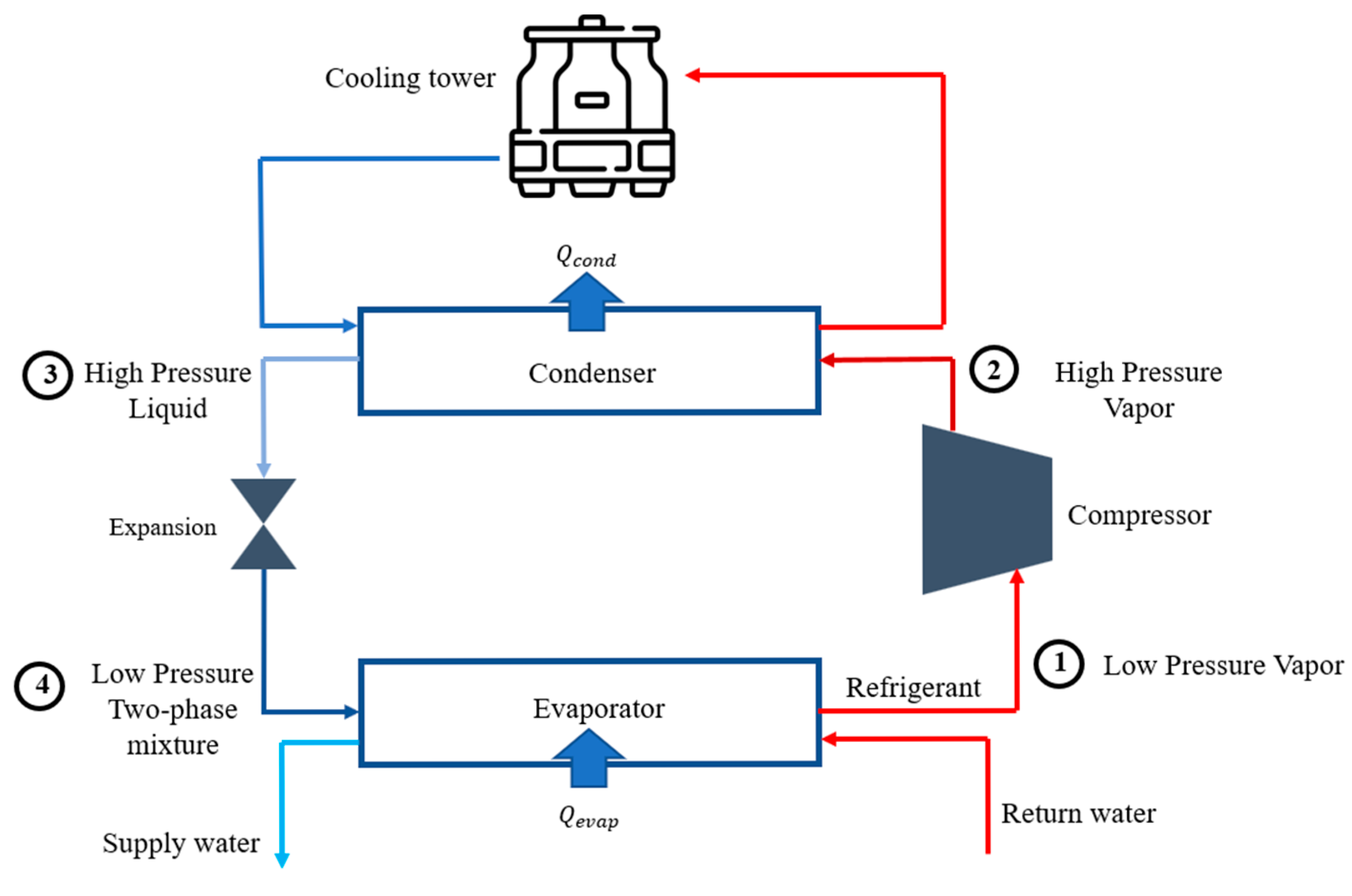
Figure 1. Water-cooled chiller schematic.
Electronics 15 00208 g001
Figure 2. Most commonly used and selected variables for chiller FDD.
Electronics 15 00208 g002
Figure 3. An overview of the proposed methodology.
Electronics 15 00208 g003
Figure 4. ASHRAE chiller system setup [56].
Electronics 15 00208 g004
Figure 5. VMD-KPCA methodology flow chart for (a) training and (b) testing phases.
Electronics 15 00208 g005
Figure 6. Feature selection framework.
Electronics 15 00208 g006
Figure 7. Plot of heat balance (a) Original data (b) Decomposed data into low (denoised) and high frequency (noise).
Electronics 15 00208 g007
Figure 8. Box plot showing the range of variables and potential outliers.
Electronics 15 00208 g008
Figure 9. Comparison of Low-Frequency (denoised) Heat Balance Data: With and Without Outlier Removal.
Electronics 15 00208 g009
Figure 10. Comparing SPE charts (a) PCA (b) VMD-PCA (c) KPCA (d) VMD-KPCA.
Electronics 15 00208 g010
Figure 11. Variation in MAR + FAR with increasing number of features for all faults at SL-1—Case 1.
Electronics 15 00208 g011
Figure 12. Deviation of refrigerant leakage fault from normal behavior for selected variables: (a) average difference, (b) average percentage error, (c) normalized difference, and (d) standard deviation of variables.
Electronics 15 00208 g012aElectronics 15 00208 g012b
Figure 13. Variation in MAR + FAR with increasing number of features for all faults at SL-1—Case 2.
Electronics 15 00208 g013
Table 1. PCA-based methods and variables used for chiller FDD.
FDD MethodReferencePCA Type/Detection/Diagnosis MethodVariables
Traditional PCAChen and Lan [21]PCA/SPE/-TWEO, TWEI, TREO, TREI,
TRCI, TRCO, TACI, TACO
Beghi et al. (2016) [22]PCA/SPE, T 2 /Reconstruction based contributionTWEO-TWEI, T s h s u c , TCA, TEA, Overall evaporator heat loss coefficients,   η p o l y , η i s e , C B E x , η c a l
Cotrufo and Zmeureanu [36]PCA/score values out of ellipsoid threshold on normal data/- T o a , P c o m p ,   i n (kW), TWEO, TWEI, TWCO, T C T S , C T V F D
PCA variantsSimmini et al. [37]Local PCA/ φ (combined of SPE and T 2 )/-TWEO-TWEI, T o a , VL, PRC, EEV, p l r c o m p r e x , P c o m p r e x :   k W
Xia et al. [38]KECA/Cauchy–Schwarz (CS) divergence/-All 64 variables reported in ASHARE RP-1043
Simmini et al. [39]KPCA/SPE/-Cond Tons, Evap Tons, P c o m p ,   i n (kW),
η c a l (kW/ton), TEA, TCA, PRE, PRC,
T R C s u b , T s h s u c , T s h d i s , P O n e t ,
T O s u m p T O f e e d , TWCO-TWCI,
TWEO-TWEI, Overall condenser heat loss coefficients, Overall evaporator heat loss coefficients
Lu et al. (2024) [40]KECA/LOF/-TWEI, TWEO, TWCI, TWCO, P c o m p ,   i n (kW), TEA, TCA, TRE, TRC, T R C s u b , T s u c , T s h s u c , T R d i s , T s h d i s , T O s u m p , P O f e e d
Hybrid of PCA and other techniquesLi et al. (2016) [41]PCA and SVDD/Distance based statisticsTWEO, TWCI, TWCO, TEA, TCA, T R C s u b , T R d i s , T O s u m p
Wang et al. [42]PCA-BNN/Posterior probabilitiesTWEI, TWEO, TWCI, TWCO, TEA, TCA, T R C s u b , T R d i s , T O s u m p
Gao et al. [43]ICA/ I 2 and dynamic thresholding using EWMA/KNN on residual vectors TWEO, TWCI, TWCO, TEA, TCA, T R C s u b , T R d i s , T O s u m p , TWEI, P c o m p ,   i n (kW), TRE, TRC, T s u c , T s h s u c , T s h d i s , T O f e e d
Table 2. Overview of supervised methods adopted for selecting key Features for Chiller FDD.
RefMachine Learning ModelsFeatures
Han et al. [46] GA-SVMTWEO, TWCO, TRC, T R d i s , TWI, P O f e e d , FWC, VE
Yan et al. [28]SVM P O f e e d , TWCO, Evap Tons, TWEI, TCA, T O s u m p , PRE, THI, TWEO, FWC, PRC, FWE, T R s u b
Gao et al. [47]RF, KNN, SVM P O f e e d , TWI, TWEO, TCA, P c o m p ,   i n (kW), PRC, T O f e e d , FWC, FWE, (Cond Tons, Evap Tons, Energy Balance, Heat Balance, Cooling Tons)
Wang et al. [48]GA-BN, BPNN, RF, CNN, SVM, RNN, AE P c o m p ,   i n (kW), TWCO, TEA, TCA, T W E I T W E O , T W C O T W C I TCA,   T W C O T W C I , Tsh_dis, T R C s u b , T O s u m p , P O f e e d , FWC, FWE,
TWCO, TCA, T W C O T W C I  
, T O s u m p , P O f e e d , FWC, FWE, ε s a t ,   e , ε s h ,   e , P c
Bi et al. [49]SVM, DT, KNN, RF, XGBoost, CatBoost, LightGBM, DNN, CNN, DBNTWI, P O f e e d , VE, VC, TCA, FWC, T O f e e d , T O s u m p , FWE, TWEO
Table 3. Initial feature subsets for cases 1 and 2.
VariablesCase 1 (Features Used and Selected in the Literature)Case 2 (Variables and Sensors Commonly Installed in the Field)
TCA
TWEO
TWCO
P O f e e d
T O s u m p
FWC
TEA
FWE
P c o m p ,   i n (kW)
TWEI
T R d i s
T R C s u b
PRC
T s h d i s
T s h s u c
TWCI
T O f e e d
TRC
TWCO-TWCI
Evap Tons
TWEO-TWEI
PRE
Cond Tons
TRE
η c o m p (kW/Ton)
T s u c
VE
Cooling Tons
P O n e t
VC
COP
P l i f t
Heat Balance (kW)
ε s a t , e = T W E I T W E O T W E I T R E
ε s h , e = T s h s u c T W E I T R E
ε s a t , c = T W C O T W C I T R C T W C I
ε s h , c = T s h d i s T R d i s T W C O
ε s u b , c = T R C s u b T R C T W C I
L M T D e = T W E I T W E O ln T W E I T R E T W E O T R E
L M T D c = T W C O T W C I ln T R C T W C I T R C T W C O
✓ indicates the selected variable.
Table 4. Features selection sequence and the associated fault detection accuracy for each fault at 1-SL.
NoFeaturesNumber of PCFDA of Each Fault
CFRLRefoverREWRCWNCGExoil
1FWC161.670.264.454.5510058.5258.52
2FWC, Cond Tons216.350.133.918.7610020.4830.09
3FWC, Cond Tons, TRC530.959.540.625.2110036.8332.4
4FWC, Cond Tons, TRC, PRC481.787.720.986.7110027.9682.13
5FWC, Cond Tons, TRC, PRC, TEA586.992.537.790.4110042.3387.13
6FWC, Cond Tons, TRC, PRC, TEA, Cooling Tons890.996.557.991.8910059.7792.11
7FWC, Cond Tons, TRC, PRC, TEA, Cooling Tons, Heat Balance 99296.96292.710070.4892.37
8FWC, Cond Tons, TRC, PRC, TEA, Cooling Tons, Heat Balance, TWCI992.497.058994.3110099.0194.42
9FWC, Cond Tons, TRC, PRC, TEA, Cooling Tons, Heat Balance, TWCI, P O n e t 910097.89278.98100100100
10FWC, Cond Tons, TRC, PRC, TEA, Cooling Tons, Heat Balance, TWCI, P O n e t , T O s u m p 1010096.988.774.73100100100
11FWC, Cond Tons, TRC, PRC, TEA, Cooling Tons, Heat Balance, TWCI, P O n e t , T O s u m p , TWEO-TWEI710097.198.977.62100100100
Table 5. Features selected sequentially from the list of Case 2 and fault detection accuracy for each fault at 1-SL.
NoFeaturesNumber of PCFDA for Each Fault
RLRefoverRCWREWCFNCGExoil
1 ε s a t , c 131.3579.4735.0417.910.5310021.76
2 ε s a t , c , TWCO346.6291.8835.8917.7623.6610027.75
3 ε s a t , c , TWCO,
L M T D c
551.795.8861.2521.927.6810042.54
4 ε s a t , c , TWCO,
L M T D c , TEA
663.9798.4362.5631.3137.810040.63
5 ε s a t , c , TWCO,
L M T D c , TEA, T s h d i s
759.4995.7147.246.8940.7410011.23
6 ε s a t , c , TWCO,
L M T D c , TEA, T s h d i s , η c o m p (kW/Ton)
774.459346.681.1981.7910032.91
7 ε s a t , c , TWCO,
L M T D c , TEA, T s h d i s , η c o m p (kW/Ton),
ε s u b , c
984.492.7967.7685.5684.8910046.08
8 ε s a t , c , TWCO,
L M T D c , TEA, T s h d i s , η c o m p (kW/Ton),
ε s u b , c , P l i f t
1090.8892.2564.8280.5278.5310044.36
9 ε s a t , c , TWCO,
L M T D c , TEA, T s h d i s , η c o m p (kW/Ton),
ε s u b , c , P l i f t , P c o m p ,   i n (kW)
995.5995.7174.686.983.0310057
10 ε s a t , c , TWCO,
L M T D c , TEA, T s h d i s , η c o m p (kW/Ton),
ε s u b , c , P l i f t , P c o m p ,   i n (kW), PRC
1095.6794.8877.6892.9181.7710049.94
11 ε s a t , c , TWCO,
L M T D c , TEA, T s h d i s , η c o m p (kW/Ton), ε s u b , c , P l i f t , P c o m p ,   i n (kW), PRC, TRC
1095.1995.0975.7191.7587.6910068.61
Disclaimer/Publisher’s Note: The statements, opinions and data contained in all publications are solely those of the individual author(s) and contributor(s) and not of MDPI and/or the editor(s). MDPI and/or the editor(s) disclaim responsibility for any injury to people or property resulting from any ideas, methods, instructions or products referred to in the content.