
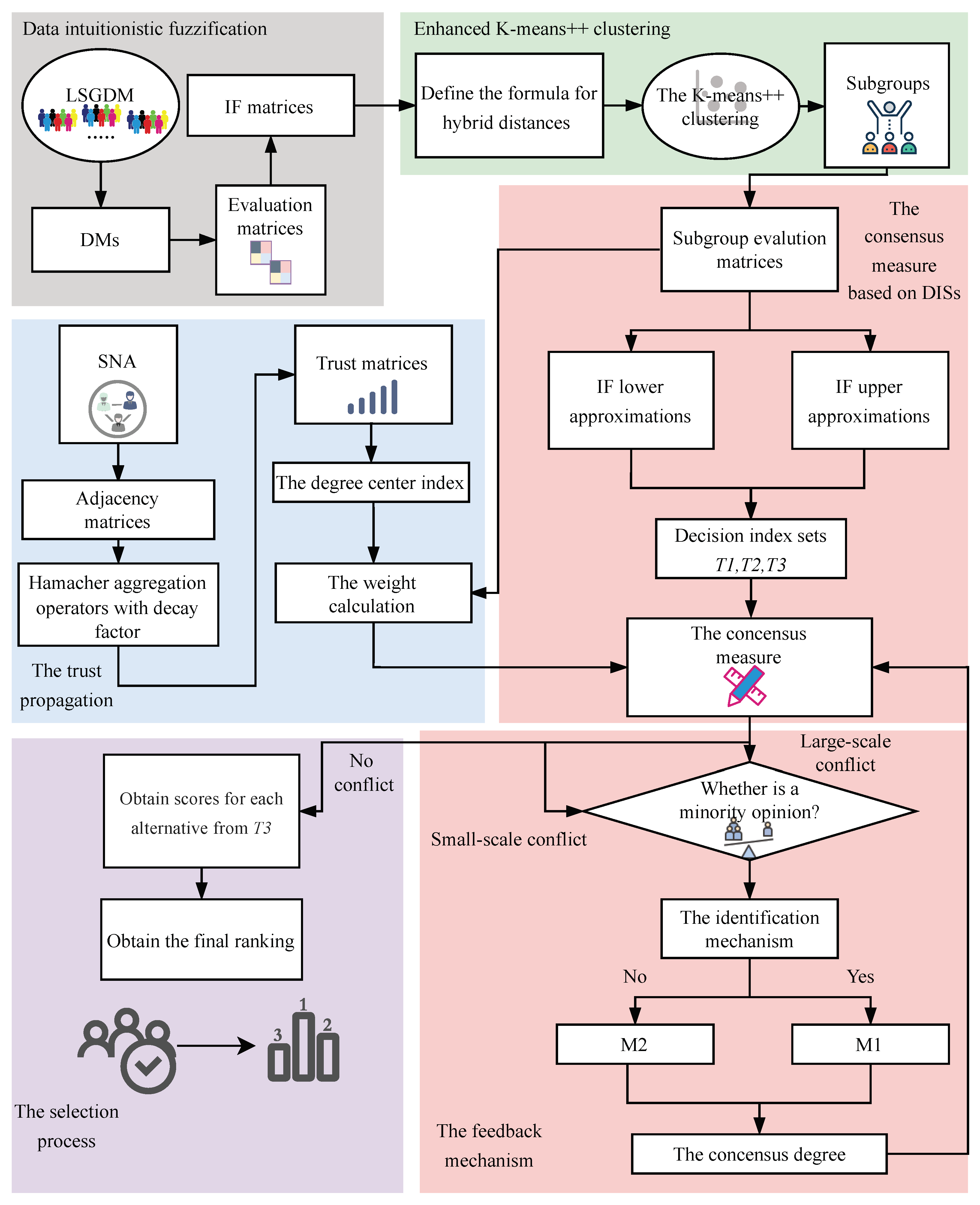
Building Consensus with Enhanced K-means++ Clustering: A Group Consensus Method Based on Minority Opinion Handling and Decision Indicator Set-Guided Opinion Divergence Degrees


Abstract
1. Introduction
1.1. Trust Propagations in SN-LSGDM
1.2. Enhancements in K-means++ Clustering Methods
1.3. CRP in LSGDM
1.4. Case Study Context in UAVs
1.5. Summary of Our Method
- (1)
- In SN-LSGDM, DMs may be influenced by their social neighbors or experience hesitation during the evaluation process. Therefore, examining their behavioral patterns within SNs is crucial. While various trust propagation operators have been proposed to enhance the decision process, existing methods for handling missing values often rely on simple statistical estimations, which introduce bias and lack interpretability. Hence, developing a propagation algorithm that not only improves the decision accuracy, but also enhances the interpretability is essential for completing trust matrices.
- (2)
- Most existing clustering methods [27] primarily focus on a single influencing factor, which often leads to suboptimal or even contradictory clustering results. To overcome this limitation, it is necessary to design a more robust clustering method that integrates two key influencing factors, ensuring greater accuracy and consistency in clustering outcomes.
- (3)
- The consensus measurement plays a pivotal role in CRP. Current methods typically determine consensus levels by setting predefined thresholds, which are often subjective. Therefore, developing a more objective and formula-driven measurement approach is essential for improving fairness and reliability in consensus assessment.
- (4)
- Existing methods for managing minority opinions generally rely on analyzing subjective discussions to assess their significance. However, given the inherent uncertainty and risk in real-world decision-making, a trust-based detection and weight-management approach can provide a more effective solution for evaluating and integrating minority opinions in the decision process.
- (1)
- The completion of incomplete trust matrices: combining the Hamacher aggregation operator with a decay factor to handle missing values in incomplete trust matrices.
- (2)
- Enhanced K-means++ clustering: integrating both cardinal and ordinal distance metrics to develop a personalized distance formula for the classical K-means++ algorithm. An advanced weighting method is proposed, considering the number of DMs and trust levels within the community.
- (3)
- The objective consensus measurement: introducing a DIS for conflict detection, offering a high level of objectivity and fairness in determining whether consensus has been reached.
- (4)
- The management of minority opinions: developing an improved method for identifying and adjusting minority opinions, leveraging group trusts to assess their importance and adjusting their weights accordingly.
2. Preliminaries
2.1. A Dynamic Consensus-Driven Framework for LSGDM
- (1)
- The meaning of sentiment scores: let the raw sentiment score , where indicates extreme the positivity and indicates extreme the negativity.
- (2)
- The decomposition of bipolar affective measures: positive certainty: ; negative skepticism: .
- (3)
- The quantification of cognitive uncertainty: certainty index (confidence in affective judgment): .
- (4)
- The synthesis of IFNs: the final IFN triplet is constructed via certainty-modulated fusion: ; .
2.2. IFNs
2.2.1. The Basic Concept of IFNs
2.2.2. IF Operations
2.2.3. IF Comparison Rules
2.3. SNA
2.3.1. The Basic Concept of SNs
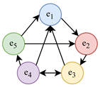
- (1)
- The graph representation: A graph is used to model the trust network among members, where nodes represent individuals, and directed edges denote trust relationships. Specifically, an edge indicates a direct trust relationship from to .
- (2)
- The algebraic representation: This method differentiates various types of relationships and demonstrates how these relationships can be combined for analysis.
- (3)
- The sociometric representation: Trust relationships between members are expressed in a matrix , where each element indicates the presence or absence of a direct trust relationship. Specifically, if , it represents a direct trust relationship from to . Conversely, if , it signifies the lack of such a relationship.
2.3.2. Hamacher Aggregation Operator
2.4. Theoretical Synthesis of Prospect and Regret Mechanisms
- Monotonicity: .
- Diminishing sensitivity: .
- Sign-dependent interpretation: signifies rejoicing, otherwise regret.
3. Clustering and Calculating Weights
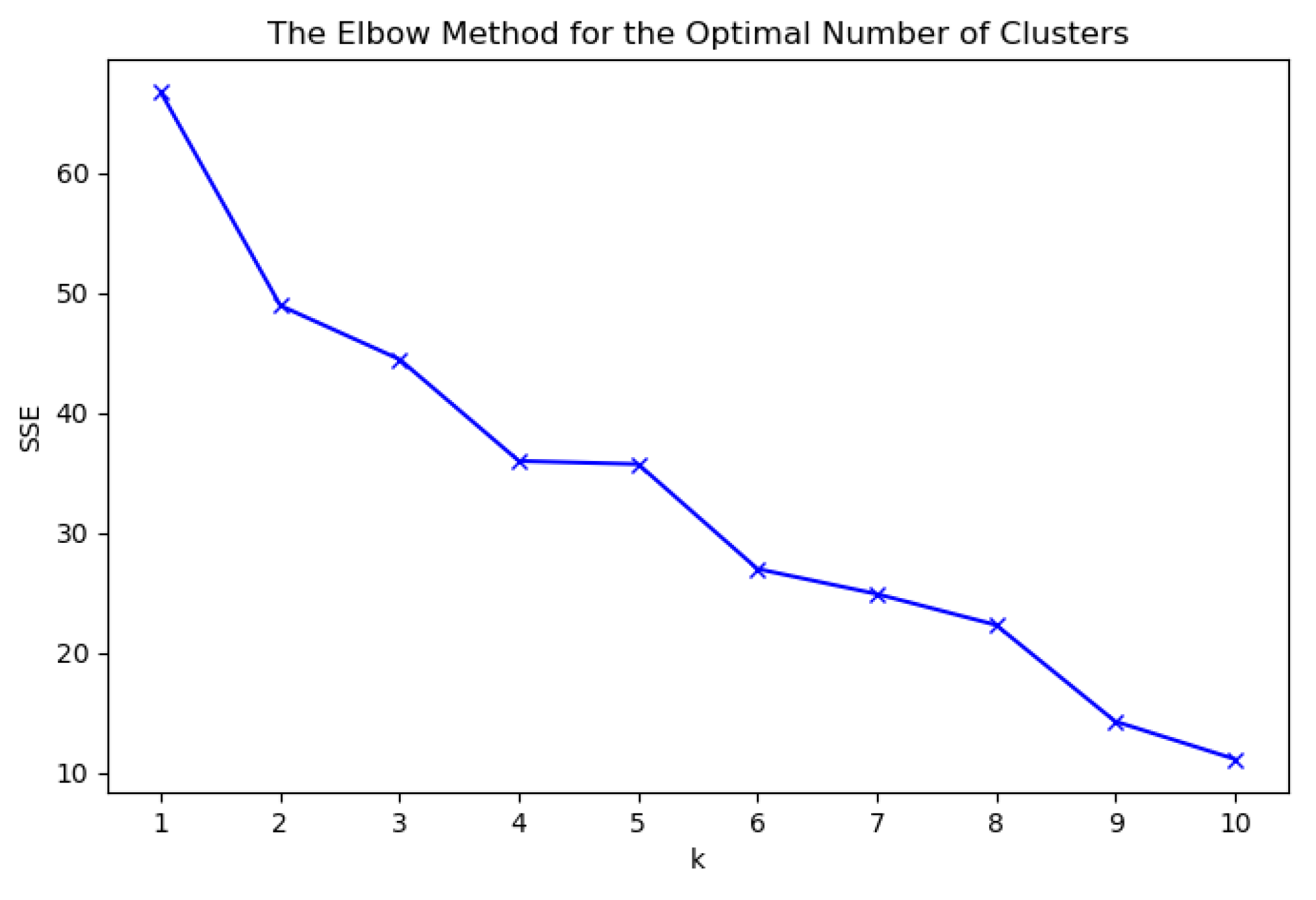
3.1. Enhanced K-means++ Clustering
3.1.1. A Hybrid Distance Metric Integrating Cardinal and Ordinal Distances
- indexes the ordinal position in the ranking;
- The indicator function is defined as:
3.1.2. K-means++ Clustering
| Algorithm 1 Enhanced K-means++ clustering with hybrid features |
| Input: The DM evaluation matrix set , the attribute weight W. |
| Output: The subgroup partition result . |
| Step 1: Data preprocessing |
| Compute the alternative sorting vector for all DMs using Equation (19); |
| Construct the mixed feature space: ; |
| Step 2: Determine the number of clusters |
| Initialize , the SSE list; |
| for to do |
| Perform standard K-means++ clustering; |
| Compute within-cluster squared error using Equation (22); |
| end for |
| Determine the optimal k value using the elbow method; |
| Step 3: Mixed distance clustering |
| Initialize cluster centers (density peak selection); |
| while not converged do |
| for each DM do |
| Compute the mixed distance to each cluster center using Equation (21); |
| Assign to the nearest cluster; |
| end for |
| Update cluster centers (weighted IF averaging); |
| end while |
3.2. Weight Determination Framework
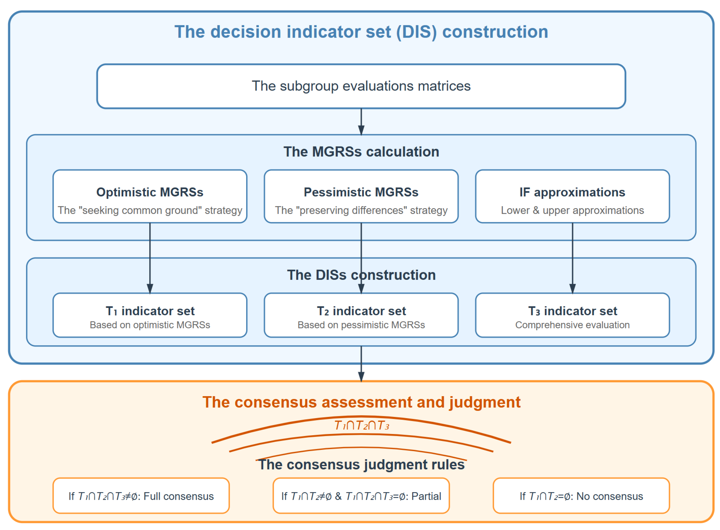
4. A CRP Method Based on MOH and DISs
4.1. Consensus Measurement
- 1.
- Optimistic MGRS—based on the ”seeking common ground while preserving differences” strategy, this model defines rough set approximations in a more inclusive manner, allowing for flexibility in classification.
- 2.
- Pessimistic MGRS—rooted in the ”seeking common ground while rejecting differences” approach, this model applies stricter constraints to ensure a higher level of consistency across granular structures.
- (1)
- If holds, then consensus has been reached.
- (2)
- If and both hold, then consensus partially reach consensus.
- (3)
- If and both hold, then consensus has not been reached.
4.2. MOH (M1)
4.2.1. Detection Mechanism
- (1)
- The consensus level of and its alignment with the group opinion are the lowest.
- (2)
- consists of a limited number of DMs. the minority opinion should satisfy the threshold , (where [.] is a floor function).
- (3)
- should hold a relatively high level of authority and gain recognition and trust from the majority of DMs within the group.
4.2.2. Management Mechanism
4.3. Opinion Divergence-Driven Dynamic Weight Adjustment (M2)
- (1)
- The subgroup reference point definition using Equation (37):
- Note: Dynamically generated from subgroup historical evaluations.
- (2)
- The prospect-deviation calculation using Equation (38):
- Function: Quantifies deviation from reference standards.
- (1)
- The nonlinear value function using Equation (14):
- (2)
- The social comparison regret value using Equation (15):
- (3)
- The integrated prospect value using Equation (41):
- (1)
- The dynamic weight update using Equation (42):
- Parameter: (recommended initial value: 0.2).
- (2)
- The weight normalization using Equation (43):
| Algorithm 2 A CRP method based on DISs and MOH |
| Input: The subgroup partition , the initial weights , the initial target matrix B. |
| Output: The final ranking . |
| Step 1: The consensus measurement |
| repeat |
| Compute MGRS indicators: , , using Equations (32)–(34); |
| until convergence condition met; |
| Step 2: Minority opinion handling |
| if then |
| Identify the candidate minority subgroups using Equation (35); |
| for each do |
| if credibility verification passes then |
| Adjust subgroup weights using Equation (36); |
| else |
| Start Step 3; |
| end if |
| end for |
| end if |
| Step 3: Dynamic weight update |
| Compute the subgroup foreground-regret value using Equation (41); |
| Update the weight using Equation (42); |
| Normalize weights using Equation (43); |
| Step 4: Target matrix evolution |
| Update the consensus matrix B using Equations (44) and (45); |
| Step 5: Generate results |
| Acquire the comprehensive score from ; |
| return ranking the result . |
5. Empirical Validation and Analysis
5.1. Empirical Validation
- (1)
- Round 1After testing, it is concluded using Equation (35) that there are minorities in subgroup 1 and subgroup 2. The management mechanism is implemented for the groups with minorities, the weights are adjusted by Equation (36), and the final weights of the subgroups are obtained as shown in Table 8. The target matrix B is updated by using the weights. After obtaining the new target matrix B, the degree of consensus is re-measured.
5.2. Sensitivity Analysis
5.3. Simulation Analysis
5.4. Comparison Analysis
5.4.1. Component Necessity Analysis via Ablation Study
5.4.2. Comparative Analysis of Trust Propagation Operators
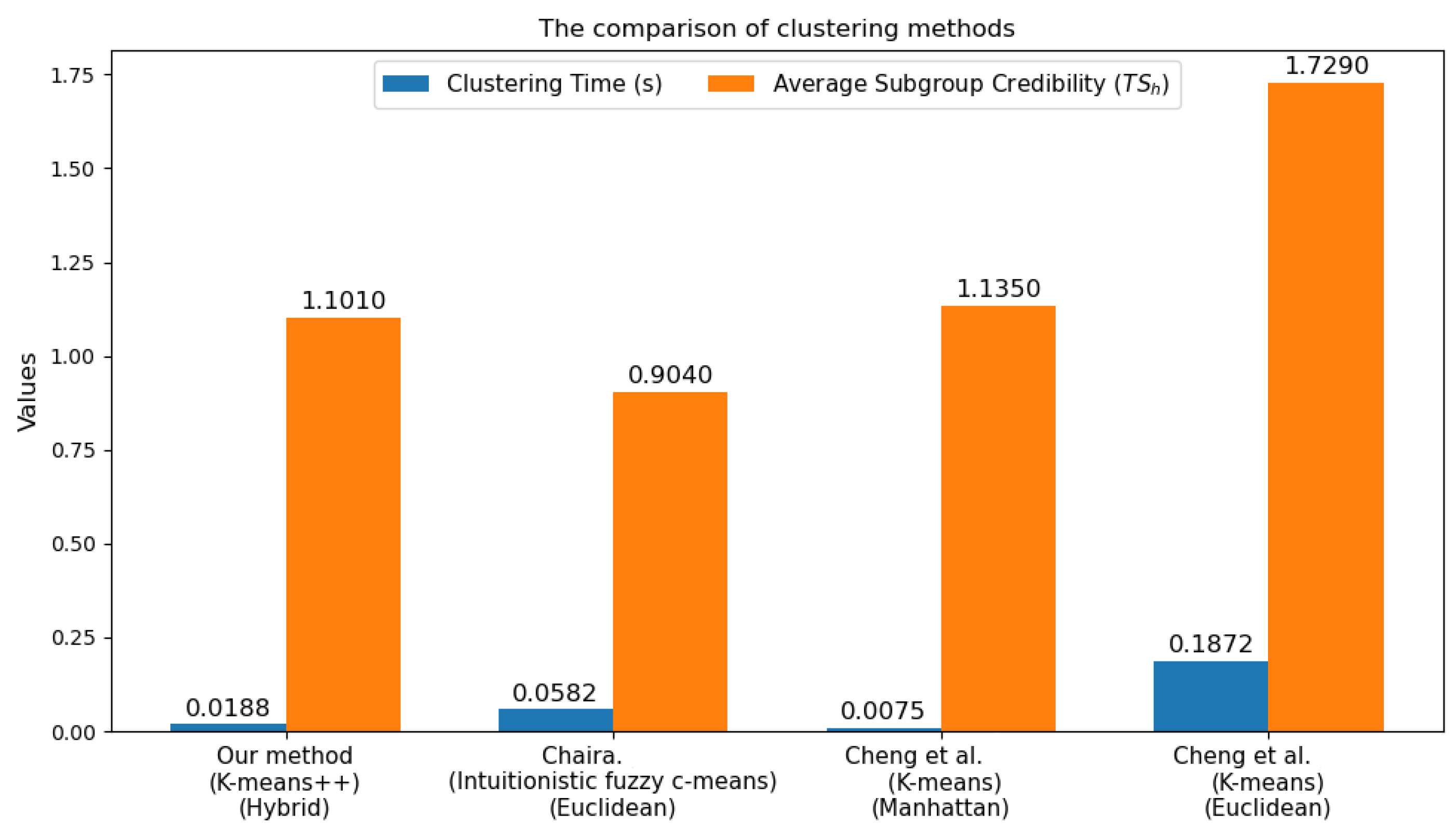
5.4.3. Comparison Among Different Clustering Methods
5.4.4. Comparison Between the Proposed Method and Existing Consensus Models
6. Conclusions
- (1)
- The proposed method leverages the Hamacher aggregation operator with a decay factor to effectively complete incomplete trust matrices while mitigating biases inherent in traditional statistical imputation. This approach enhances the interpretability and reliability of trust relationships in SNs.
- (2)
- By integrating hybrid distance metrics (Euclidean, Manhattan, and Hamming distances) into the K-means++ algorithm, we achieve fine-grained clustering of DMs. This multidimensional strategy accounts for both evaluation data and preference rankings, significantly improving subgroup homogeneity and reducing computational complexity.
- (3)
- A DIS grounded in MGRSs provides a robust, formula-driven mechanism for assessing consensus levels. By replacing subjective thresholds with granular approximations, this method ensures fairness and transparency in conflict detections.
- (4)
- A systematic mechanism for detecting and adjusting minority opinions is proposed, incorporating subgroup credibility and trust centrality. This balances minority influence without over-amplification, fostering innovation while preserving decision stability.
- (1)
- The current model is demonstrated in the context of UAV selection based on structured and semi-structured data. Future extensions may consider more heterogeneous decision scenarios, such as new energy vehicles [56].
- (2)
- Although we incorporated social trust propagation, the model does not yet address trust decay over time or dynamic trust formation, which are relevant in evolving SNs.
- (3)
- While our current work integrates sentiment analysis indirectly, future implementations could enhance this component with real-time emotion detection and contextual semantic embeddings.
Author Contributions
Funding
Data Availability Statement
Conflicts of Interest
Abbreviations
| LSGDM | Large-scale group decision-making |
| DMs | Decision-makers |
| SNs | Social networks |
| SNA | Social network analysis |
| CRP | Consensus-reaching process |
| MOH | Minority opinion handling |
| DISs | Decision indicator sets |
| IFNs | Intuitionistic fuzzy numbers |
| IFSs | Intuitionistic fuzzy sets |
| SSE | Sum of squared errors |
| UAVs | Unmanned aerial vehicles |
| MGRS | Multigranulation rough set |
| TL | Traditional LSGDM models |
| SNL | Enhanced LSGDM models integrated with SN |
| ML | Behavior-management-oriented LSGDM models to handle misbehaviors |
Appendix A
| DMs’ Evaluation Matrices | |
Appendix B
| Trust Degree Matrix Among DMs (Completed) |
Appendix C
| Sub-Group Evaluation Matrices | |
References
- Kiesler, S.; Sproull, L. Group decision making and communication technology. Organ. Behav. Hum. Decis. Process. 1992, 52, 96–123. [Google Scholar] [CrossRef]
- Wang, Y.; Song, H.; Dutta, B.; García-Zamora, D.; Martínez, L. Consensus reaching in LSGDM: Overlapping community detection and bounded confidence-driven feedback mechanism. Inf. Sci. 2024, 679, 121104. [Google Scholar] [CrossRef]
- Tang, M.; Liao, H. From conventional group decision making to large-scale group decision making: What are the challenges and how to meet them in big data era? A state-of-the-art survey. Omega 2021, 100, 102141. [Google Scholar] [CrossRef]
- Zhang, C.; Wang, Y.; Sangaiah, A.; Alenazi, M.J.F.; Aborokbah, M. An incomplete three-way consensus algorithm for unmanned aerial vehicle purchase using optimization-driven sentiment analysis. Future Gener. Comput. Syst. 2025, 107761. [Google Scholar] [CrossRef]
- Garcia-Zamora, D.; Labella, A.; Ding, W.; Rodríguez, R.M.; Martínez, L. Large-scale group decision making: A systematic review and a critical analysis. IEEE/CAA J. Autom. Sin. 2022, 9, 949–966. [Google Scholar] [CrossRef]
- Li, X. Big data-driven fuzzy large-scale group decision making (LSGDM) in circular economy environment. Technol. Forecast. Soc. Change 2022, 175, 121285. [Google Scholar]
- Shen, Y.; Ma, X.; Xu, Z.; Herrera-Viedma, E.; Maresova, P.; Zhan, J. Opinion evolution and dynamic trust-driven consensus model in large-scale group decision-making under incomplete information. Inf. Sci. 2024, 657, 119925. [Google Scholar] [CrossRef]
- Mahmoudi, A.; Abbasi, M.; Yuan, J.; Li, L. Large-scale group decision-making (LSGDM) for performance measurement of healthcare construction projects: Ordinal Priority Approach. Appl. Intell. 2022, 52, 13781–13802. [Google Scholar] [CrossRef]
- Zhang, R.; Huang, J.; Xu, Y. Consensus models with aggregation operators for minimum quadratic cost in group decision making. Appl. Intell. 2023, 53, 1370–1390. [Google Scholar] [CrossRef]
- Wang, Y.; He, S.; Zamora, D.; Pan, X.; Martínez, L. A large scale group three-way decision-based consensus model for site selection of new energy vehicle charging stations. Expert Syst. Appl. 2023, 214, 119107. [Google Scholar] [CrossRef]
- Xu, T.; He, S.; Yuan, X.; Zhang, C. Enhancing group consensus in social networks: A two-stage dual-fine tuning consensus model based on adaptive Leiden algorithm and minority opinion management with non-cooperative behaviors. Electronics 2024, 13, 4930. [Google Scholar] [CrossRef]
- Hsieh, Y.; Lu, L.; Ku, Y. Review evaluation for hotel recommendation. Electronics 2023, 12, 4673. [Google Scholar] [CrossRef]
- Tian, X.; Ma, W.; Wu, L.; Xie, M.; Kou, G. Large-scale consensus with dynamic trust and optimal reference in social network under incomplete probabilistic linguistic circumstance. Inf. Sci. 2024, 661, 120123. [Google Scholar] [CrossRef]
- Harshavardhan, A.; Boyapati, P.; Neelakandan, S.; Abdul-Rasheed Akeji, A.A.; Singh Pundir, A.K.; Walia, R. LSGDM with Biogeography-Based Optimization (BBO) Model for Healthcare Applications. J. Healthc. Eng. 2022, 2022, 2170839. [Google Scholar] [CrossRef]
- Chunaev, P. Community detection in node-attributed social networks: A survey. Comput. Sci. Rev. 2020, 37, 100286. [Google Scholar] [CrossRef]
- Jin, F.; Cai, Y.; Zhou, L.; Ding, T. Regret–rejoice two-stage multiplicative DEA models-driven cross-efficiency evaluation with probabilistic linguistic information. Omega 2023, 117, 102839. [Google Scholar] [CrossRef]
- Wu, J.; Chiclana, F.; Fujita, H.; Herrera-Viedma, E. A visual interaction consensus model for social network group decision making with trust propagation. Knowl.-Based Syst. 2017, 122, 39–50. [Google Scholar] [CrossRef]
- Liu, B.; Zhou, Q.; Ding, R.X.; Palomares, I.; Herrera, F. Large-scale group decision making model based on social network analysis: Trust relationship-based conflict detection and elimination. Eur. J. Oper. Res. 2019, 275, 737–754. [Google Scholar] [CrossRef]
- Liu, P.; Li, Y.; Wang, P. Social trust-driven consensus reaching model for multiattribute group decision making: Exploring social trust network completeness. IEEE Trans. Fuzzy Syst. 2023, 31, 3040–3054. [Google Scholar] [CrossRef]
- Chu, J.; Wang, Y.; Liu, X.; Liu, Y. Social network community analysis based large-scale group decision making approach with incomplete fuzzy preference relations. Inf. Fusion 2020, 60, 98–120. [Google Scholar] [CrossRef]
- Xu, Y.; Li, C.; Wen, X. Missing values estimation and consensus building for incomplete hesitant fuzzy preference relations with multiplicative consistency. Int. J. Comput. Intell. Syst. 2018, 11, 101–119. [Google Scholar] [CrossRef]
- Song, Y.; Li, G. Handling group decision-making model with incomplete hesitant fuzzy preference relations and its application in medical decision. Soft Comput. 2019, 23, 6657–6666. [Google Scholar] [CrossRef]
- Liu, P. Some Hamacher aggregation operators based on the interval-valued intuitionistic fuzzy numbers and their application to group decision making. IEEE Trans. Fuzzy Syst. 2013, 22, 83–97. [Google Scholar] [CrossRef]
- Ren, Y.; Pu, J.; Yang, Z.; Xu, J.; Li, G.; Pu, X.; Yu, P.S.; He, L. Deep clustering: A comprehensive survey. IEEE Trans. Neural Netw. Learn. Syst. 2024, 36, 5858–5878. [Google Scholar] [CrossRef]
- Xu, D.; Tian, Y. A comprehensive survey of clustering algorithms. Ann. Data Sci. 2015, 2, 165–193. [Google Scholar] [CrossRef]
- Wang, Y.; Qian, J.; Hassan, M.; Zhang, X.; Zhang, T.; Yang, C.; Zhou, X.; Jia, F. Density peak clustering algorithms: A review on the decade 2014–2023. Expert Syst. Appl. 2024, 238, 121860. [Google Scholar] [CrossRef]
- Kapoor, A.; Singhal, A. A comparative study of K-Means, K-Means++ and Fuzzy C-Means clustering algorithms. In Proceedings of the 2017 3rd International Conference on Computational Intelligence & Communication Technology (CICT), Ghaziabad, India, 9–10 February 2017; pp. 1–6. [Google Scholar]
- Hajihosseinlou, M.; Maghsoudi, A.; Ghezelbash, R. Intelligent mapping of geochemical anomalies: Adaptation of DBSCAN and mean-shift clustering approaches. J. Geochem. Explor. 2024, 258, 107393. [Google Scholar] [CrossRef]
- Cheng, F. A comparative study of the performance of Spark-based k-means algorithm based on Euclidean distance and Manhattan distance. In Proceedings of the 2024 3rd International Conference on Big Data, Information and Computer Network (BDICN), Sanya, China, 12–14 January 2024; pp. 1–6. [Google Scholar]
- Guo, L.; Zhan, J.; Zhang, C.; Xu, Z. A large-scale group decision-making method fusing three-way clustering and regret theory under fuzzy preference relations. IEEE Trans. Fuzzy Syst. 2023, 32, 4846–4860. [Google Scholar] [CrossRef]
- Labella, A.; Liu, H.; Rodríguez, R.M.; Martínez, L. A cost consensus metric for consensus reaching processes based on a comprehensive minimum cost model. Eur. J. Oper. Res. 2020, 281, 316–331. [Google Scholar] [CrossRef]
- Zou, W.; Wan, S.; Dong, J.; Martínez, L. A new social network driven consensus reaching process for multi-criteria group decision making with probabilistic linguistic information. Inf. Sci. 2023, 632, 467–502. [Google Scholar] [CrossRef]
- Tang, M.; Liao, H.; Mi, X.; Lev, B.; Pedrycz, W. A hierarchical consensus reaching process for group decision making with noncooperative behaviors. Eur. J. Oper. Res. 2021, 293, 632–642. [Google Scholar] [CrossRef]
- Cheng, X.; Zhang, K.; Wu, T.; Xu, Z.; Gou, X. An opinions-updating model for large-scale group decision-making driven by autonomous learning. Inf. Sci. 2024, 662, 120238. [Google Scholar] [CrossRef]
- Gai, T.; Wu, J.; Cao, M.; Liu, Y.; Liang, C. Blockchain platform selection for supply chain finance: A bilateral-negotiation-based group multiattribute decision making method. IEEE Trans. Comput. Soc. Syst. 2024, 11, 6072–6086. [Google Scholar] [CrossRef]
- Zhang, X.; Liu, Q.; Zhang, C.; Zhan, J. New fuzzy rough set models based on implication operators. Comput. Appl. Math. 2025, 44, 125. [Google Scholar] [CrossRef]
- Laor, T. Breaking the silence: The role of social media in fostering community and challenging the spiral of silence. Online Inf. Rev. 2024, 48, 710–724. [Google Scholar] [CrossRef]
- Ren, R.; Tang, M.; Liao, H. Managing minority opinions in micro-grid planning by a social network analysis-based large scale group decision making method with hesitant fuzzy linguistic information. Knowl.-Based Syst. 2020, 189, 105060. [Google Scholar] [CrossRef]
- Xu, X.; Du, Z.; Chen, X. Consensus model for multi-criteria large-group emergency decision making considering non-cooperative behaviors and minority opinions. Decis. Support Syst. 2015, 79, 150–160. [Google Scholar] [CrossRef]
- Liu, P.; Li, Y.; Wang, P. Opinion dynamics and minimum adjustment-driven consensus model for multi-criteria large-scale group decision making under a novel social trust propagation mechanism. IEEE Trans. Fuzzy Syst. 2022, 31, 307–321. [Google Scholar] [CrossRef]
- Chaira, T. A novel intuitionistic fuzzy C means clustering algorithm and its application to medical images. Appl. Soft Comput. 2011, 11, 1711–1717. [Google Scholar] [CrossRef]
- Shen, Y.; Ma, X.; Zhang, H.; Zhan, J. Fusion social network and regret theory for a consensus model with minority opinions in large-scale group decision making. Inf. Fusion 2024, 112, 102548. [Google Scholar] [CrossRef]
- Zhang, Z.; Xu, Y.; Hao, W.; Yu, X. A signed network analysis-based consensus reaching process in group decision making. Appl. Soft Comput. 2021, 100, 106926. [Google Scholar] [CrossRef]
- Zhang, H.; Palomares, I.; Dong, Y.; Wang, W. Managing non-cooperative behaviors in consensus-based multiple attribute group decision making: An approach based on social network analysis. Knowl.-Based Syst. 2018, 162, 29–45. [Google Scholar] [CrossRef]
- Tan, C.; Yi, W.; Chen, X. Hesitant fuzzy Hamacher aggregation operators for multicriteria decision making. Appl. Soft Comput. 2015, 26, 325–349. [Google Scholar] [CrossRef]
- Liu, X.; Yang, Y.; Jiang, J. The behavioral TOPSIS based on prospect theory and regret theory. Int. J. Inf. Technol. Decis. Mak. 2023, 22, 1591–1615. [Google Scholar] [CrossRef]
- Bisht, G.; Pal, A.K. Prospect–regret theory based decision-making approach for incomplete probabilistic hesitant fuzzy environment: An application to medical field. Expert Syst. Appl. 2024, 250, 123906. [Google Scholar] [CrossRef]
- Kahneman, D.; Tversky, A. Prospect theory: An analysis of decision under risk. In Handbook of the Fundamentals of Financial Decision Making: Part I; World Scientific: Hackensack, NJ, USA, 2013; pp. 99–127. [Google Scholar]
- Zhang, S.; Zhu, J.; Liu, X.; Chen, Y. Regret theory-based group decision-making with multidimensional preference and incomplete weight information. Inf. Fusion 2016, 31, 1–13. [Google Scholar] [CrossRef]
- Li, R.; Zhang, C.; Li, D.; Li, W.; Zhan, J. Improved evidential three-way decisions in incomplete multi-scale information systems. Int. J. Approx. Reason. 2025, 181, 109417. [Google Scholar] [CrossRef]
- Yuan, X.; Xu, T.; He, S.; Zhang, C. An online review data-driven fuzzy large-scale group decision-making method based on dual fine-tuning. Electronics 2024, 13, 2702. [Google Scholar] [CrossRef]
- Chen, G.; Wei, L.; Fu, J.; Li, C.; Zhao, G. A large group emergency decision-making method based on uncertain linguistic cloud similarity method. Math. Comput. Appl. 2022, 27, 101. [Google Scholar] [CrossRef]
- Meng, F.; Tang, J.; An, Q. Cooperative game based two-stage consensus adjustment mechanism for large-scale group decision making. Omega 2023, 117, 102842. [Google Scholar] [CrossRef]
- Liang, X.; Guo, J.; Liu, P. A large-scale group decision-making model with no consensus threshold based on social network analysis. Inf. Sci. 2022, 612, 361–383. [Google Scholar] [CrossRef]
- Liu, Z.; Wang, W.; Zhang, X.; Liu, P. A dynamic dual-trust network-based consensus model for individual non-cooperative behaviour management in group decision-making. Inf. Sci. 2024, 674, 120750. [Google Scholar] [CrossRef]
- Ding, J.; Zhang, C.; Li, D.; Li, W.; Zhan, J. A three-way large-scale group decision-making method integrating sentiment analysis and quantum interference-based prospect theory for the selection of new energy vehicles. Expert Syst. Appl. 2025, 275, 126940. [Google Scholar] [CrossRef]


| Mathematical Symbols | Meaning |
|---|---|
| The set of experts | |
| The decision-making matrix of a DM | |
| The set of attributes | |
| Attributes weights | |
| The set of alternatives | |
| The trust matrix | |
| The fuzzy number trust degree matrix | |
| The credibility measure of a subgroup | |
| The score value related to a DM | |
| The representation form of an IFN | |
| The set of subgroups | |
| The index related to positive certainty | |
| The index related to negative suspicion | |
| The evaluation matrix after subgroup aggregations |
| Graph | Algebraic | Sociometric |
|---|---|---|
 | , , , , , , , , |
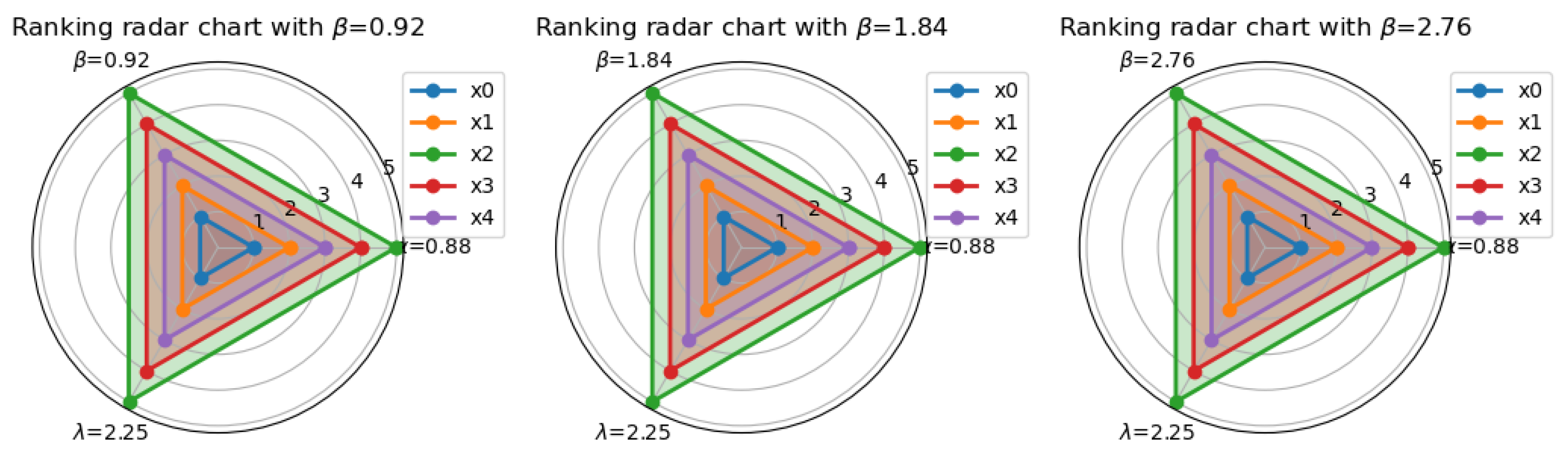
| Symbols | Keys | Behavioral Interpretations |
|---|---|---|
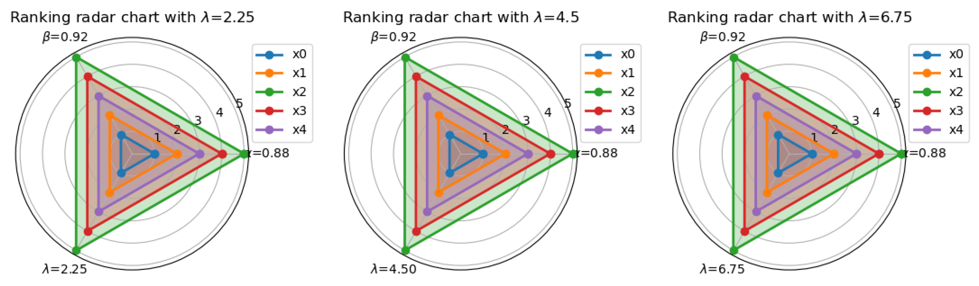
| 0.88 | Risk sensitivity in gains | |
| Loss aversion magnitude | ||
| Loss amplification factor | ||
| 0.2 | Regret aversion intensity |
| The Grouping of DMs |
|---|
| Weights of DMs |
|---|
| 0.062 0.065 0.081 0.072 0.079 |
| 0.067 0.096 0.080 0.072 0.067 |
| 0.091 0.090 0.078 |
| # | |||
|---|---|---|---|
| G0 | 6 | 1.889 | 0.044 |
| G1 | 1 | 6.612 | 0.833 |
| G2 | 2 | 3.606 | 0.082 |
| G3 | 4 | 2.204 | 0.041 |
| Indexes | Values | The Greatest Subset |
|---|---|---|
| 0.057 | 0.070 | 0.603 | 0.270 |
| Indexs | Values | The Greatest Subset |
|---|---|---|
| {1,4} | ||
| {1,4} | ||
| {1,4} |
| Ranking Results |
|---|
| Our method | |
|---|---|
| Our method eliminates the ranking relationship. | |
| Our method eliminates MOH | |
| Our method replaces DIS with weighted sum during decision-making | |
| Our method eliminates prospect–regret theory |
| Methods | Total Execution Time | Clustering Time | Initial Consensus Degree | Final Ranking |
|---|---|---|---|---|
| 0.0234 s | 0.0188 s | Partial contradiction | ||
| 0.0091 s | 0.0045 s | Partial contradiction |
| Methods | CRP Time | Number of Iterations | Final Sorting Result |
|---|---|---|---|
| 0.0046 s | 1 | ||
| 0.0012 s | 1 |
| Methods | The CRP Time | The Final Sorting Result |
|---|---|---|
| 0.0046 s | ||
| 0.0054 s |
| Methods | CRP Time | Number of Iterations | Final Sorting Result |
|---|---|---|---|
| 0.0046 s | 1 | ||
| 0.0032 s | 4 |
| Our method | Our proposed method, which integrates the Hamacher aggregation operator with a decay factor to dynamically refine trust values, accounting for both multiplicative interactions and distance-dependent decay in SNs. | |
| Weighted averaging | A classical approach that estimates missing trust values using weighted averages of direct and indirect trust relationships, without explicit decay modeling. | |
| Heuristic operators | A heuristic-based method that prioritizes short propagation paths but lacks a systematic framework for decay factor adjustment. |
| Methods | Relative Error | Average Time/Iteration (s) | Decay Modeling Support |
|---|---|---|---|
| 0.9992 | 0.00124 | Yes | |
| 1.3994 | 0.00005 | No | |
| 2.5137 | 0.00153 | No |
| Types | References | Trust Propagation | Clustering Based on Hybrid Distance | DIS | MOH | Managing Opinions with Reference to Trust |
|---|---|---|---|---|---|---|
| TL | Yuan et al. [51] | No | No | No | Yes | No |
| Chen et al. [52] | No | No | No | No | Yes | |
| Meng et al. [53] | No | No | No | No | No | |
| SNL | Liang et al. [54] | No | No | No | Yes | Yes |
| Liu et al. [19] | No | No | No | Yes | Yes | |
| ML | Liu et al. [55] | Yes | No | Yes | Yes | Yes |
| Xu et al. [39] | Yes | No | Yes | Yes | No | |
| Xu et al. [11] | No | No | Yes | Yes | No | |
| Our method | Yes | Yes | Yes | Yes | Yes |
Disclaimer/Publisher’s Note: The statements, opinions and data contained in all publications are solely those of the individual author(s) and contributor(s) and not of MDPI and/or the editor(s). MDPI and/or the editor(s) disclaim responsibility for any injury to people or property resulting from any ideas, methods, instructions or products referred to in the content. |
© 2025 by the authors. Licensee MDPI, Basel, Switzerland. This article is an open access article distributed under the terms and conditions of the Creative Commons Attribution (CC BY) license (https://creativecommons.org/licenses/by/4.0/).
Share and Cite
Hou, X.; Xu, T.; Zhang, C. Building Consensus with Enhanced K-means++ Clustering: A Group Consensus Method Based on Minority Opinion Handling and Decision Indicator Set-Guided Opinion Divergence Degrees. Electronics 2025, 14, 1638. https://doi.org/10.3390/electronics14081638
Hou X, Xu T, Zhang C. Building Consensus with Enhanced K-means++ Clustering: A Group Consensus Method Based on Minority Opinion Handling and Decision Indicator Set-Guided Opinion Divergence Degrees. Electronics. 2025; 14(8):1638. https://doi.org/10.3390/electronics14081638
Chicago/Turabian StyleHou, Xue, Tingyu Xu, and Chao Zhang. 2025. "Building Consensus with Enhanced K-means++ Clustering: A Group Consensus Method Based on Minority Opinion Handling and Decision Indicator Set-Guided Opinion Divergence Degrees" Electronics 14, no. 8: 1638. https://doi.org/10.3390/electronics14081638
APA StyleHou, X., Xu, T., & Zhang, C. (2025). Building Consensus with Enhanced K-means++ Clustering: A Group Consensus Method Based on Minority Opinion Handling and Decision Indicator Set-Guided Opinion Divergence Degrees. Electronics, 14(8), 1638. https://doi.org/10.3390/electronics14081638