Multi-Strategy Improved Aquila Optimizer Algorithm and Its Application in Railway Freight Volume Prediction

Abstract

This study proposes a multi-strategy improved Aquila optimizer (MIAO) to address the key limitations of the original Aquila optimizer (AO). First, a phasor operator is introduced to eliminate excessive control parameters in the X2 phase, transforming it into an adaptive parameter-free process. Second, a flow direction operator enhances the X3 phase by improving population diversity and local exploitation. The MIAO algorithm is applied to optimize Long Short-Term Memory (LSTM) hyperparameters, forming the MIAO_LSTM model for monthly railway freight forecasting. Comprehensive evaluations on 15 benchmark functions show MIAO’s superior performance over SOA, PSO, SSA, and AO. Using freight data (2005–2021), MIAO_LSTM achieves lower MAE, MSE, and RMSE compared to traditional LSTM and hybrid models (SSA_LSTM, PSO_LSTM, etc.). Further, Grey Relational Analysis selects high-correlation features (≥0.8) to boost accuracy. The results validate MIAO_LSTM’s effectiveness for practical freight predictions.

1. Introduction

With the continuous advancement of technology and theoretical knowledge in human society, optimization algorithms have evolved from initial derivative-based methods to become derivative-free meta-heuristic intelligent algorithms. This evolution has significantly enhanced the ability of algorithms to handle nonlinear and convex optimization problems. In the current era, where artificial intelligence and big data are prevalent, the demand for optimization algorithms across various industries is increasingly growing. However, the optimization capabilities of different algorithms vary when applied to specific problems. Consequently, a considerable number of scholars are engaged in developing new algorithms or refining existing ones to enhance their accuracy and convergence speed, tailoring them to address distinct challenges. For example, Wu et al. proposed an enhanced AO algorithm improved by PSO to address the UAV path planning problem [1]. Experimental results also demonstrated the practicality of PSAO in UAV path planning. Anirban et al. employed the Aquila optimizer (AO) algorithm to optimize the selection and placement of distributed generators (DG) [2]. This approach demonstrates the effectiveness of AO in addressing complex optimization problems in power system planning. Chiheb et al. enhanced the Aquila optimizer (AO) algorithm by incorporating Cauchy mutation and successfully applied it to the classification of brain tumor data [3]. Furthermore, numerous studies have demonstrated that combining optimization algorithms with neural network models can significantly enhance the overall performance of the algorithms [4,5,6,7,8]. For example, Qiao et al. combined an improved Aquila optimizer with temporal convolutional networks and random forests to form a meta-heuristic deep learning model, demonstrating the effectiveness of the algorithm in rainfall-runoff prediction [9]. Duan et al. proposed a hybrid model integrating a fully convolutional neural network (FCN) and the Aquila optimizer (AO) to predict solar radiation intensity, offering valuable insights for clean energy utilization [10]. These studies represent specific applications of optimization algorithms in various fields. Compared with other deep learning architectures (e.g., CNN), Long Short-Term Memory (LSTM) networks demonstrate superior capability in modeling temporal dependencies within sequential data. Therefore, this study proposes a novel MIAO-LSTM hybrid model that integrates an enhanced Aquila optimizer (improved through phasor and flow direction operators) with an LSTM network for railway freight volume prediction in China.

With the rapid development of the logistics industry, optimization algorithms and deep learning models have demonstrated their significant importance in research related to freight volume prediction. There are also further studies on rail freight volume forecasting. Xu et al. [11] combined the product seasonal model with the LSTM that introduces the attention mechanism, and used the error correction method to improve the poor prediction accuracy of the product seasonal model, which improved the model’s data processing capability compared with the traditional LSTM network. Seock et al. [12] used PCA to complete the screening of input data for the situation of low freight volume data and large data fluctuations. Feng et al. [13] used a capsule neural network algorithm to predict the export demand of the China–Europe liner; the difference with the completely connected neural network is that the capsule neural network adds two coupling coefficients in the stage of input linear weighted summation, which further strengthens the model’s nonlinear fitting ability. Also, to reduce the possible impact of the gradient problem, the capsule neural network optimizes the activation function, which also improves the prediction accuracy. However, these two initiatives reduce the speed of training the model, as well as the adaptability of the model with more input data.

Railway freight is a complex nonlinear system, which is jointly influenced by numerous factors, but the above studies do not consider the influencing factors, and only use the past freight volume data to predict the future freight volume, which is the prediction from the freight volume to the freight volume, with a large uncertainty and a large fluctuation in the prediction results [13,14]. Railway freight, as a large-capacity, long-distance, low-cost mode of transport, has a natural advantage in terms of the transportation of bulk commodities, which leads to the railway being used to transport bulk commodities. National policies have a greater impact, therefore, most scholars will use the production of coal, crude oil, and other types of bulk commodities, and other modes of transport that have a competitive relationship with railway freight, for freight volume forecasting. The influence of these factors has resulted in a large number of studies and has achieved excellent research results. For example, Liu et al. [15] used grey correlation analysis to select the features with higher correlation from the numerous influencing factors. Zhang et al. [16] proposed a multidimensional LSTM prediction model to synchronize data with different attributes of spatial and temporal correlation, considering that railway freight traffic is affected by a variety of factors. The advantage of this model is that it can reflect correlations between data in different dimensions. While these studies have scientifically predicted results for freight traffic, it remains unconvincing that most hyperparameters in algorithmic models are set empirically.

To increase the reliability of the prediction model, numerous experts and scholars in the field of transportation at home and abroad have combined the optimization algorithm with the machine learning model and used the optimization algorithm to optimize the hyperparameters of the model and reduce the influence of subjective factors. For example, in marine ship trajectory prediction, Liu et al. [17] proposed a deep learning-based ship trajectory prediction framework (QSD_LSTM), which incorporated the dynamic QSD algorithm into the LSTM network, and this model improved the prediction accuracy while making it easier to represent the occurrence of trajectory conflicts, which improved the efficiency of intelligent supervision at sea. In terms of passenger flow prediction, Qin et al. [18], based on the passenger flow, which has a nonlinear and seasonal trend, used STL to decompose the data into seasonal, trend component, and residual component, and used the improved grasshopper optimization algorithm to predict the trend and residual, respectively, and, finally, the results of the three parts were added to obtain the monthly passenger flow prediction results. This combination of a decomposition and optimization algorithm reduced the influence of noise information and has great scalability. Similarly, in air cargo prediction, Li et al. [19] used the VMD technique to decompose dynamic and nonlinear air cargo data, extracted the main features of the original data, and eliminated the noise, after which the generated high-frequency components were decomposed twice with an EMD optimized Elman’s network structure using a cuckoo optimization algorithm, and each component was predicted with this model, which technically found the effective data. The critical point of the lag region improves the performance of the prediction method. In terms of traffic flow prediction, Manuel et al. [20] combined a convolutional neural network and a bidirectional LSTM network to form a CNN_BILSTM prediction model, which combined the ability of CNN to extract hidden valuable features from the input and the ability of Bi-LSTM to address the continuity of information in time-series data, which is of some reference value for coping with traffic congestion. In the area of waterborne freight activity prediction, Bhurtyal et al. [21] leveraged near real-time vessel tracking data from the Automatic Identification System (AIS) data set. Long Short-Term Memory (LSTM), Temporal Convolutional Network (TCN), and Temporal Fusion Transformer (TFT) machine learning models are developed using the features extracted from the AIS and the historical WCS data. The output of the model is the prediction of the quarterly volume of commodities (in tons) at the port terminals for four quarters in the future. In terms of railway freight volume prediction, Yang et al. [22] constructed four prediction models based on multivariate statistical methods, which are of some reference value in terms of freight vehicles and labor allocation.

In summary, research on freight volume forecasting has ranged from single-algorithm models, for the use of optimization algorithms to optimize model parameters and reduce human intervention to improve prediction accuracy, to the use of targeted processing and optimization methods based on different data characteristics. All these means are overcoming the limitations of the NFL theorem [23] and expanding the applicability of the models. However, different algorithms differ from each other in the same scenario. Therefore, we employ novel optimization algorithms to solve the freight volume prediction problem.

Based on the above studies, the literature on freight volume prediction is relatively thin and there is a large research space. In this paper, we use the multi-strategy modified Aquila optimizer to optimize LSTM for freight volume prediction research, and the main research contributions are as follows.

(1) The Aquila optimizer (AO) has been improved by incorporating the phasor operator and flow direction operator. The introduction of the phasor operator significantly reduces the impact of parameters on the algorithm’s performance and enhances its optimization capability, as demonstrated by benchmark test functions. The reduction in parameters increases the ability of the Aquila optimizer to handle complex nonlinear systems, such as railway freight volume prediction.

(2) The MIAO_LSTM model was applied to freight volume prediction, and the impact of influencing factors on the prediction results was investigated. Railway freight volume forecasting is jointly affected by numerous factors, and most of its input features are selected by relying on experience, which may have a certain impact on the prediction results, therefore, this paper uses Grey Relational Analysis to calculate the size of the correlation between each input feature and the freight volume, and selects the input features whose correlation is greater than 0.8 to conduct the test again. This result demonstrates that a reasonable choice of input features will also improve the prediction accuracy of freight volume.

The remainder of this paper is structured as follows: Section 2 introduces the LSTM network model; Section 3 presents the multi-strategy improved Aquila optimizer (MIAO) algorithm; and Section 4 applies the constructed MIAO_LSTM model to railway freight volume prediction, further validating the effectiveness of the MIAO model. This section provides a detailed explanation of the model’s inputs and outputs, its construction, and the analysis of prediction results. Section 5 summarizes the contributions of the paper, discusses its limitations, and outlines future research directions.

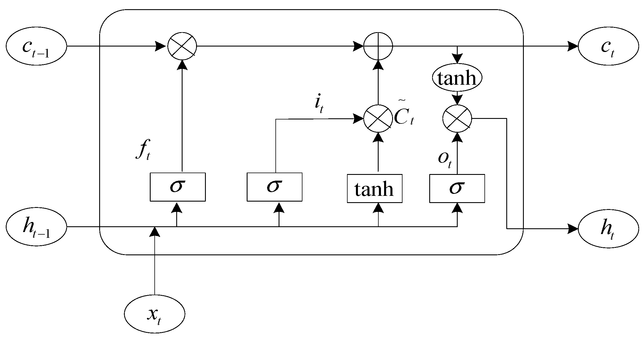
2. LSTM Neural Network

The LSTM (Long Short-Term Memory) neural network is derived from the recurrent neural network, which has achieved great results in the fields of structural modeling [24,25], engineering design [26,27], global optimization [28,29], and energy efficiency [30,31], including three gating units, namely, oblivion gate, input gate, and output gate, and the structure of the LSTM network unit is shown in Figure 1.

In the Figure, σ denotes the sigmoid activation function, c denotes the information that needs to be stored for a prolonged time, h_t−1 denotes the output information at the previous moment, h_t is the output information at the current state, and x_t denotes the current input.

In the LSTM neural network, the forgetting gate plays the role of screening information. First of all, the last moment of output information h_t−1 and the current input information x_t are combined into a new input matrix, input to the sigmoid function, and this function will be normalized to the input data between 0 and 1. At this point, the sigmoid function plays the role of a switch, and the data close to 0 “forget” to retain the data close to 1, which is the role of the LSTM forget gate.

$$f_t=\sigma (w_f\cdot [h_{t-1},x_t]+b_f)$$

(1)

In Equation (1), $w_f$ is the weight matrix of the forgetting gate and $b_f$ is the bias of the forgetting gate.

After the tanh function becomes the new candidate vector ${\tilde{C}}_t$, the previous part determines the values to be saved and discarded for the original candidate vector, and the saved values are added to the values saved in the previous state. The corresponding formula is as follows.

$$i_t=\sigma (w_i\cdot [h_{t-1},x_t]+b_i)$$

(2)

$${\tilde{C}}_t=\tanh (w_c\cdot [h_{t-1},x_t]+b_c)$$

(3)

In the above equation, $i_t$ is the output of the input matrix after the 2nd sigmoid activation function, $w_i$ and $b_i$ are the weight matrix and bias of the sigmoid function in the input gate, and $w_c$ and $b_c$ are the weight and bias of the tanh function.

Finally, the value obtained by summing the input gates is changed to [−1, 1] by the tanh function, and the value retained by the last sigmoid function is the output value at this moment. The following Equations (4) and (5) are shown.

$$o_t=\sigma (w_o\cdot [h_{t-1},x_t]+b_o)$$

(4)

$$h_t=o_t\cdot \tanh (c_t)$$

(5)

In the above equation, $o_t$ is the output value of the 3rd sigmoid function, $h_t$ is the final output of the network, and $w_o$ and $b_o$ are the weight matrix and bias of the 3rd sigmoid function.

3. Multi-Strategy Improved Aquila Optimizer

The Aquila optimizer is a current meta-heuristic optimization algorithm proposed by Laith Abualigah et al. in 2021 [32]. The algorithm builds a mathematical model by simulating four different predation strategies of Aquila, which has the advantages of quick convergence and strong global search ability, but the traditional Aquila optimizer has extra control parameters, ignores the excellent predation ability of individual Aquila, and lacks the mutual transfer of information between individuals, so the phase quantum operator and the flow direction operator are used to improve the $X_2$ and $X_3$ stages of the Aquila optimizer. The four phases of the Aquila optimizer and their improvements are described below.

$$X_1\left(t+1\right)=X_{best}\left(t\right)\cdot \left(1-{\displaystyle \frac{t}{T}}\right)+rand\cdot \left(X_M\left(t\right)-X_{best}\left(t\right)\right)$$

(6)

$$X_M\left(t\right)={\displaystyle \frac{1}{N}}{\sum }_{i=1}^N{X}_i\left(t\right),\forall j=\mathrm{1,2},\dots ,Dim$$

(7)

where $X_1\left(t+1\right)$ is the solution of the next iteration of the first stage t; $X_{best}\left(t\right)$ is the optimal solution of the t-th iteration; $X_M\left(t\right)$ denotes the average of the position of the solution at t iterations; rand denotes the random number between [0 and 1]; t is the number of current iterations; T is the maximum number of iterations; and N denotes the total number of samples. Moreover, Dim is the dimension of the problem.

3.1. Vector Operators to Improve the Aquila Optimizer

The formulas associated with the reduced exploration ($X_2$) phase of the Aquila optimizer are described below.

$$X_2\left(t+1\right)=X_{best}\left(t\right)\cdot Levy\left(D\right)+X_R\left(t\right)+rand\cdot \left(y-x\right)$$

(8)

$$Levy\left(D\right)=s\cdot {\displaystyle \frac{\mu \delta }{{\left|\upsilon \right|}^{\frac{1}{\beta }}}}$$

(9)

$$\delta =\left({\displaystyle \frac{\Gamma \left(1+\beta \right)\cdot \mathit{sin}e\left(\frac{\pi \beta }{2}\right)}{\Gamma \left(\frac{1+\beta }{2}\right)\cdot \beta \cdot 2^{\left(\frac{\beta -1}{2}\right)}}}\right)$$

(10)

$$y=r\mathit{cos}\left(\theta \right)$$

(11)

$$x=r\mathit{sin}\left(\theta \right)$$

(12)

$$r=r_1+U\cdot D_1$$

(13)

$$\theta =-\omega D_1+{\displaystyle \frac{3\pi }{2}}$$

(14)

where $X_2\left(t+1\right)$ is the solution of the next iteration of the second stage t; Levy (D) is the Levy flight distribution function; and $X_R\left(t\right)$ is a random number in the range [1, N] at t iterations. Let x and y denote the shape of the helix during the search. The letter s is a constant of 0.01; μ and υ are random numbers between 0 and 1; β has the value of 1.5; δ is computed by Equation (5); $r_1$ is a fixed search for the [1, 20] number of cycles; U is 0.00565; D₁ is an integer between [1 and Dim]; and ω is 0.005.

In phase $X_2$, the Aquila optimizer involves many control parameters. Numerous metaheuristics are highly sensitive to subtle tuning of the control parameters, which may cause the algorithm to converge prematurely or get stuck in a local optimal solution. To overcome this problem, the phase operator is introduced in the $X_2$ stage to remove the influence of the control parameters and transform this stage into a non-parametric adaptive control stage, which improves the performance of the Aquila optimizer.

The phase quantity operator [33] is derived from the theory of phase quantities in mathematics, which reduces or eliminates the control parameters of the optimization algorithm by selecting suitable operator functions through the periodic trigonometric functions sin and cos for the purpose of adaptive, non-parametric optimization. Using the intermittent characteristic of the trigonometric function, all the control parameters of the $X_2$ phase of the Aquila optimizer are represented by the phase angle θ, and the role played by the control parameters is represented by the function containing θ. For this purpose, a one-dimensional phase angle θ_i is used to represent each individual in the population, so that the i-th individual can be represented by a vector of size $\overrightarrow{X_i}\angle {\theta }_i$ and θ_i, i.e., $\overrightarrow{X_i}\angle {\theta }_i$.

The resulting phase operators are shown in Equations (15) and (16).

$$p\left({\theta }_i^t\right)={\left|\mathit{cos}{\theta }_i^t\right|}^{2\mathit{sin}{\theta }_i^t}$$

(15)

$$g\left({\theta }_i^t\right)={\left|\mathit{sin}{\theta }_i^t\right|}^{2\mathit{cos}{\theta }_i^t}$$

(16)

Equation (8) is improved by combining Equations (15) and (16), and the improved equation is shown in Equation (17).

$$X_2\left(t+1\right)=X_{best}\left(t\right)\cdot Levy\left(D\right)\cdot p\left({\theta }_i^t\right)+X_R\left(t\right)\cdot g\left({\theta }_i^t\right)$$

(17)

3.2. Flow Direction Operator to Improve the Aquila Optimizer

The formula for the development phase of the expansion is described below:

$$X_3\left(t+1\right)=\alpha \cdot \left(X_{best}\left(t\right)-X_M\left(t\right)\right)-rand+\delta \cdot \left(rand\cdot \left(UB-LB\right)+LB\right)$$

(18)

where $X_3\left(t+1\right)$ is the solution generated by $X_3$ at t + 1 iterations; UB and LB are the upper and lower bounds on the solution space, respectively; and the values of α and δ are both 0.1.

Phase $X_3$ of the Aquila optimizer is improved by using the flow direction operator, which enables information transfer between individuals. By improving the utilization of information between individuals, the optimization discovery capability of the proposed algorithm is greatly improved. The flow direction operator [34] is derived from the flow direction algorithm proposed by Hojat, which is a physically based algorithm, and the flow direction algorithm (FDA) simulates the movement state and formation process of runoff. The flow moves towards and around the lowest point, which is the optimal value of the objective function. The flow direction algorithm assumes that φ neighbors exist around each water flow and the mathematical expression of its positional relationship is shown in Equation (19).

$$Neighbor\_X_j\left(t\right)=X_i\left(t\right)+randn\cdot \Delta$$

(19)

where $Neighbor\_X_j\left(t\right)$ denotes the j-th location adjacent to $X_i\left(t\right)$, randn is a random number following a standard normal distribution, and $\Delta$ is the search radius. Equation (19) establishes a search region for each individual in the Aquila optimizer, and the size of the value $\Delta$ determines the size of the search range, within which information can be passed to each other, and the formula for $\Delta$ is shown below.

$$\Delta =\left(rand\cdot Xrand-rand\cdot X_i\left(t\right)\right)\cdot ‖X_{best}\left(t\right)-X_i\left(t\right)‖\cdot W$$

(20)

In the above equation, rand is a uniformly distributed random number, $Xrand$ is a random position generated in the search space, $X_{best}\left(t\right)$ is the optimal solution of the t-th iteration in the Aquila optimizer, and $X_i\left(t\right)$ is the current position of the i-th individual at the t-th iteration. The formula for W is as follows.

$$W=\left({\left(1-{\displaystyle \frac{t}{T}}\right)}^{2\cdot randn}\right)\cdot \left(rand\cdot {\displaystyle \frac{t}{T}}\right)\cdot rand$$

(21)

In the FDA algorithm, the flow rate of runoff to an adjacent region is directly related to its slope, and, therefore, the following relation is used to determine the flow rate vector.

$$V=rand\cdot S_0$$

(22)

where $S_0$ denotes the slope vector between the current individual and its neighbors, and the slope vector between the i-th individual and the j-th neighbor is determined by the following equation.

$$S_0\left(i,j\right)={\displaystyle \frac{X_i\left(t\right)\_fitness-Neighbor\_X_j\left(t\right)\_fitness}{‖X_i\left(t\right)-Neighbor\_X_j\left(t\right)‖}}$$

(23)

where $X_i\left(t\right)\_fitness$ denotes the target value of $X_i\left(t\right)$ and $Neighbor\_X_j\left(t\right)\_fitness$ denotes the target value of $Neighbor\_X_j\left(t\right)$.

The flow operator used in this paper is defined as follows.

$$FD=V\cdot {\displaystyle \frac{X_i\left(t\right)-Neighbor\_X_j\left(t\right)}{‖X_i\left(t\right)-Neighbor\_X_j\left(t\right)‖}}$$

(24)

The Aquila optimizer suffers from reduced population diversity and tends to get stuck in local optima at later iterations, so the flow direction operator is introduced to improve the $X_3$ phase of the Aquila optimizer. The flow algorithm allows information transfer between individuals and to each other, which improves information utilization. At the same time, the introduction of nonlinear weights W also increases the randomness of the algorithm in the late iteration, which further enhances the algorithm’s ability to search and jump out of the local optimum and improves the $X_3$ stage of the Aquila optimizer, which is also known as Equation (18), as shown in Equation (25).

$$X_3\left(t+1\right)=\left(X_{best}\left(t\right)-X_M\left(t\right)\right)+FD$$

(25)

The formulae for the reduction development stage of the Aquila optimizer are described below.

$$X_4\left(t+1\right)=QF\times X_{best}\left(t\right)-\left(G_1\times X\left(t\right)\times rand\right)-G_2\times Levy\left(D\right)+rand\times G_1$$

(26)

$$QF\left(t\right)=t^{{\displaystyle \frac{2\times rand-1}{{\left(1-T\right)}^2}}}$$

(27)

$$G_1=2\times rand-1$$

(28)

$$G_2=2\times \left(1-{\displaystyle \frac{t}{T}}\right)$$

(29)

where $X_4\left(t+1\right)$ is the solution generated by the fourth search method $X_4$ in t + 1 iterations; QF is used to balance the quality function of the search strategy; $G_1$ denotes the various motions of the AO during the hunting period; while $G_2$ is a linear function indicating the flight slope of the AO used to track the prey.

In summary, this paper adopts the phase operator to improve the $X_2$ stage of the Aquila optimizer and the flow operator to improve the $X_3$ stage, forming a multi-strategy improved Aquila optimizer, which has a faster convergence speed and a stronger anti-interference ability, compared with the traditional Aquila optimizer.

3.3. Time Complexity Analysis

According to reference [32], the time complexity of the AO algorithm depends on three aspects: population initialization, fitness calculation, and solution update. Assuming the population size is N, the spatial dimension is D, and the maximum number of iterations is T, the complexity of the population initialization process can be calculated as $O\left(N\right)$, where $O\left(T\times N\right)+O\left(T\times N\times D\right)=O\left(T\times N\times \left(D+1\right)\right)$ represents the complexity of the solution update process. Therefore, the overall time complexity of the Aquila optimizer (AO) algorithm is $O\left(N\times \left(T\times D+1\right)\right)$.

In the MIAO algorithm, the phasor operator treats each individual in the population as a one-dimensional phasor that varies randomly within the range $\left[0, 2\pi \right]$ as the iterations progress. Therefore, the time complexity of the phasor operator is $O\left(T\times N\right)$. Compared to the Aquila optimizer (AO) algorithm, the flow direction operator does not involve the population initialization process. The time complexity of the flow direction operator is $O\left(T\times N\times \left(D+1\right)\right)$. Therefore, the inclusion of the phasor operator and the flow direction operator does not increase the overall time complexity. Thus, the time complexity of MIAO remains $O\left(N\times \left(T\times D+1\right)\right)$.

3.4. Algorithm Performance Testing

To verify the effectiveness of the algorithm proposed in this paper, it is tested with the seagull optimization algorithm (SOA), particle swarm optimization (PSO), sparrow search algorithm (SSA), genetic algorithm (GA), whale optimization algorithm (WOA), and the traditional Aquila optimizer (AO) for performance testing with a uniform setting of the number of populations N = 30, the number of iterations T = 500, and the test dimensionality of 10 dimensions, and the selected test functions are shown in

Table 1. Test Functions.

Number	Function	Dim	Range of Values	Function Minimum
F1	Sphere	10	[−100, 100]	0
F2	Schwefel 2.22	10	[−10, 10]	0
F3	Schwefe l1.2	10	[−100, 100]	0
F4	Rastrigin	10	[−5.12, 5.12]	0
F5	Ackley	10	[−32, 32]	0
F6	Griewank	10	[−600, 600]	0
F7	Shekel’s	2	[−65, 65]	1
F8	Kowalik	4	[−5, 5]	0.0003
F9	Shekel	4	[0, 10]	−10.1532

,

Table 2. CEC2017 Test Functions.

Number	Function	Dim	Function Minimum
F10	Hybrid Function 1 (N = 3)	10	1100
F11	Hybrid Function 2 (N = 3)	10	1200
F12	Hybrid Function 3 (N = 3)	10	1300

and

Table 3. CEC2022 Test Functions.

Number	Function	Dim	Function Minimum
F13	Shifted and full Rotated Zakharov Function	10	300
F14	Shifted and full Rotated Rosenbrock’s Function	10	400
F15	Shifted and full Rotated Rastrigin’s Function	10	600

.

To ensure that the experimental results are scientifically sound, nine test functions were chosen to test the performance of these algorithms. The algorithms are written in MatlabR2020a and the experimental environment was equipped with an AMD R7 3.2 GHz CPU sourced from the United States, 8.00 GB RAM, and the Windows11 operating system. Each experiment is run independently for 30 epochs, where F1–F3 are 3 unimodal test functions to test the global exploration capability of the algorithm. F4–F6 are 3 multi-peak test functions to test the exploitation capability of the algorithm. F7–F9 are 3 fixed-dimensional multi-peak test functions to check the exploration capability of the algorithm in a low-dimensional search space.

3.5. Optimized Accuracy Analysis

The MIAO algorithm and SOA, PSO, SSA, AO, GA, and WOA are run independently on the above nine test functions for 30 times, the experimental results are recorded, and the optimal value, average value, and standard deviation of each algorithm are taken as the evaluation indexes, and the test results are shown in

Table 4. Test function results (Dim = 10).

Function	Indicator	SOA	PSO	SSA	AO	GA	WOA	MIAO
F1	Min	0.9747	2.2776 × 10−3	9.0612 × 10−94	8.0671 × 10−154	5.6596 × 10−5	0.0177	0
	Avg	1.7663	2.7648 × 10−5	5.1241 × 10−92	4.5553 × 10−153	5.6620 × 10−5	0.0181	0
	Std	0.6617	9.1205 × 10−6	6.1442 × 10−94	3.2478 × 10−156	3.1114 × 10−7	9.8454 × 10−5	0
F2	Min	0.5083	0.0076	8.0319 × 10−73	1.9341 × 10−74	61.8327	3.8565	2.7518 × 10−163
	Avg	1.7572	0.0468	4.6704 × 10−32	9.2415 × 10−72	61.8537	3.8573	3.2224 × 10−159
	Std	1.1509	0.0346	6.8445 × 10−32	1.4256 × 10−72	0.3365	0.0220	6.4513 × 10−160
F3	Min	318	1.7363 × 10−4	7.9068 × 10−41	7.0266 × 10−144	2.2291 × 104	7.8134	2.4477 × 10−290
	Avg	1.5844 × 104	2.6250 × 10−4	2.1716 × 10−27	3.2245 × 10−131	2.2308 × 104	7.8174	5.8713 × 10−280
	Std	3.5224 × 107	1.9794 × 10−4	3.7729 × 10−27	6.2884 × 10−131	139.9352	0.0451	1.2223 × 10−280
F4	Min	2.8017	3.9936	0	0	305.1149	57.6735	0
	Avg	15.8255	8.9826	0	0	305.2132	57.7261	0
	Std	20.9482	2.5335	0	0	1.7705	0.3725	0
F5	Min	0.0043	0.0066	8.8818 × 10−16	8.8818 × 10−16	12.0512	1.1865	8.8818 × 10−16
	Avg	0.2709	0.4557	8.8818 × 10−16	8.8818 × 10−16	12.0517	1.1877	8.8818 × 10−16
	Std	0.3008	0.5398	0	0	0.0776	0.0060	0
F6	Min	1.1445 × 10−6	1.0639 × 10−5	0	0	76.9796	0.0049	0
	Avg	1.5935	3.0234 × 10−3	0	0	76.9967	0.0049	0
	Std	1.4952	6.2142 × 10−3	0	0	0.4964	2.5043 × 10−5	0
F7	Min	2.1994	12.6705	2.9821	0.9980	0.9980	12.6505	0.998
	Avg	5.8792	12.6705	2.5631	0.9980	0.9989	12.6709	0.998
	Std	5.1739	0	1.3330	0	0.0052	0.0511	0
F8	Min	0.0083	6.7822 × 10−4	3.0749 × 10−3	5.6790 × 10−4	3.0743 × 10−4	5.5682 × 10−4	3 × 10−4
	Avg	0.0080	9.1594 × 10−4	7.0122 × 10−3	8.9940 × 10−4	3.0749 × 10−4	5.5707 × 10−4	3.0783 × 10−4
	Std	0.0053	5.7354 × 10−4	4.7752 × 10−3	3.1122 × 10−4	1.6726 × 10−4	2.7375 × 10−6	9.2314 × 10−6
F9	Min	−9.8922	−5.0522	−10.1532	−10.1532	−10.1532	−5.1357	−10.1532
	Avg	−9.3907	−5.0522	−10.1532	−10.1527	−10.1532	−5.1285	−10.1532
	Std	0.4532	0	0	0.2140	0	0.0259	0
F10	Min	1129.3641	1164.2365	1154.446	1254.0563	1869.6077	1147.1684	1118.1889
	Avg	1327.626	1205.3622	1197.6151	1547.6576	2256.957	1212.4352	1123.0806
	Std	253.9851	256.8852	52.3607	436.2854	459.9986	260.3948	23.2064
F11	Min	3.2748 × 106	29,785.211	8.9678 × 105	3.7546 × 105	1.6506 × 108	2.3763 × 106	6631.6392
	Avg	5.2157 × 107	32,566.241	4.1196 × 106	5.6649 × 106	2.3036 × 108	2.9092 × 106	8612.8511
	Std	8.3428 × 107	8577.025	6.0351 × 106	41,277.025	1.5203 × 108	3.2845 × 106	5715.0389
F12	Min	2881.1053	3219.9767	1861.3017	3932.2987	8127.2746	2355.4759	2296.0489
	Avg	9560.7322	6259.8794	2117.5401	4499.4024	15,189.909	5570.1388	6854.7878
	Std	8026.6254	5674.9556	2652.4021	5631.2648	12,744.508	6243.5142	5254.3974
F13	Min	3003.448	671.7705	300	3459.4516	22,562.931	10,929.078	300
	Avg	4483.3896	948.664	300	4752.7466	36,962.052	20,147.071	300
	Std	2364.0351	563.8855	0	1807.5991	30,221.552	155,022.034	0
F14	Min	463.2278	467.0899	412.372	415.3034	741.6854	477.5774	407.6572
	Avg	475.8909	506.3929	431.9853	421.8737	814.4241	481.5953	418.6846
	Std	18.3624	50.3625	26.0324	16.3202	152.6747	8.2152	15.3203
F15	Min	609.1434	600.1775	623.4102	613.5755	644.9434	639.5955	600.1775
	Avg	614.0139	611.0127	640.1609	617.8035	680.2351	669.3752	611.0127
	Std	15.0557	24.9527	36.3021	10.5526	153.6620	40.9988	24.9527

below. The values in bold in the table are the optimal results.

As can be seen from Table 4, the proposed multi-strategy modified Aquila optimizer shows significant improvement in finding the optimal action for the three unimodal test functions F1–F3, and MIAO is robust. Moreover, MIAO is able to find the theoretical optimal value on the two multi-peak test functions F4 and F6, which indicates that MIAO has excellent evasion performance, does not easily get trapped in the local optimal solution, and has strong anti-stagnation performance. In the last three fixed-dimensional multi-peak test functions, MIAO also has the best optimization search performance and can essentially find its theoretical optimum, indicating the superior global search capability of the multi-strategy modified Aquila optimizer. F10–F15 represent six CEC benchmark test functions, which were used to further validate the optimization capability of MIAO. Experimental results also demonstrate that, compared to AO, MIAO exhibits superior optimization performance.

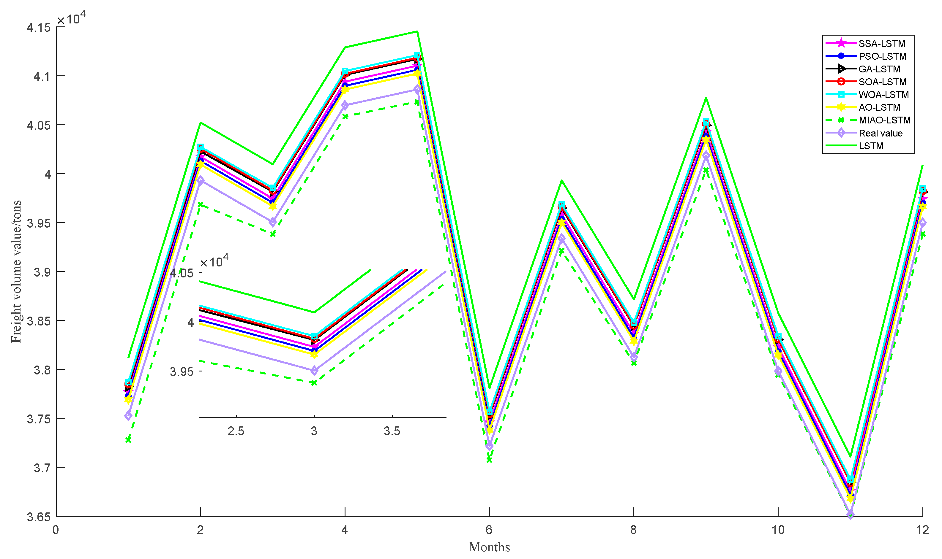
3.6. Convergence Curve Analysis

Figure 2 shows the convergence performance analysis of SOA, PSO, SSA, AO, GA, WOA, and MIAO for 10 dimensions and 500 iterations of the pairwise function optimization procedure. It can be visualized from Figure 2 that MIAO has the fastest convergence rate and the highest convergence accuracy among the 15 tested functions. This indicates that MIAO has superior low-dimensional spatial exploration ability to the other six algorithms.

3.7. Wilcoxon Rank-Sum Test

The Wilcoxon rank-sum test [35] is a non-parametric statistical method used to determine whether there are significant differences between two samples. In this study, the Wilcoxon rank-sum test was employed on nine classical benchmark functions to assess whether the MIAO algorithm exhibits significant differences compared to the other six algorithms. Here, p represents the test result and h indicates the significance judgment result. When p < 0.05, h = 1 signifies that the MIAO algorithm is significantly stronger than the other algorithms. When p > 0.05, h = 0 indicates that the MIAO algorithm is significantly weaker than the other algorithms. When p is displayed as N/A, it means that the significance test cannot be performed, suggesting that the significance of the MIAO algorithm may be equivalent to that of the other algorithms. The results are shown in

Table 5. The results of the rank-sum test.

Function	SOA		PSO		SSA		AO		GA		WOA
	p	h	p	h	p	h	p	h	p	h	p	h
F1	1.7265 × 10−4	1	1.7265 × 10−4	1	1.7265 × 10−4	1	1.7265 × 10−4	1	1.7265 × 10−4	1	1.7265 × 10−4	1
F2	1.7265 × 10−4	1	1.7265 × 10−4	1	1.7265 × 10−4	1	1.7265 × 10−4	1	1.7265 × 10−4	1	1.7265 × 10−4	1
F3	1.7265 × 10−4	1	1.7265 × 10−4	1	1.7265 × 10−4	1	1.7265 × 10−4	1	1.7265 × 10−4	1	1.7265 × 10−4	1
F4	6.3352 × 10−4	1	6.3352 × 10−4	1	N/A	0	N/A	0	6.3352 × 10−4	1	6.3352 × 10−4	1
F5	6.3352 × 10−4	1	6.3352 × 10−4	1	N/A	0	N/A	0	6.3352 × 10−4	1	6.3352 × 10−4	1
F6	6.3864 × 10−5	1	6.3864 × 10−5	1	N/A	0	N/A	0	6.3864 × 10−5	1	6.3864 × 10−5	1
F7	2.0525 × 10−3	1	2.0525 × 10−3	1	2.0525 × 10−3	1	N/A	0	2.0525 × 10−3	1	2.0525 × 10−3	1
F8	6.3864 × 10−5	1	6.3864 × 10−5	1	6.3864 × 10−5	1	6.3864 × 10−5	1	6.3864 × 10−5	1	6.3864 × 10−5	1
F9	0.007936	1	0.007936	1	0.007936	1	0.007936	1	0.007936	1	0.007936	1

.

3.8. Ablation Experiment

To further validate the effectiveness of the proposed improvements and investigate the impact of each enhancement strategy on the algorithm’s optimization performance, this study conducts comparative experiments on nine classical benchmark functions. The algorithms compared include the original Aquila optimizer (AO), the AO enhanced with the phasor operator (PAO), the AO enhanced with the flow direction operator (FAO), and the AO improved with multiple strategies (MIAO). The experimental results are shown in

Table 6. Optimization Results of Different Strategies.

Function	Indicator	AO	PAO	FAO	MIAO
F1	Min	8.0671 × 10−154	1.0306 × 10−311	3.919 × 10−2835	0
	Avg	4.5553 × 10−153	9.6317 × 10−304	1.5095 × 10−183	0
	Std	3.2478 × 10−156	5.3267 × 10−304	3.2056 × 10−183	0
F2	Min	1.9341 × 10−74	2.0326 × 10−108	6.9102 × 10−96	2.7518 × 10−163
	Avg	9.2415 × 10−72	9.0651 × 10−106	3.7549 × 10−83	3.2224 × 10−159
	Std	1.4256 × 10−72	8.0255 × 10−106	4.2256 × 10−83	6.4513 × 10−160
F3	Min	7.0266 × 10−144	1.2792 × 10−281	4.8584 × 10−147	2.4477 × 10−290
	Avg	3.2245 × 10−131	7.6 × 10−280	1.2243 × 10−139	5.8713 × 10−280
	Std	6.2884 × 10−131	5.3624 × 10−280	1.2898 × 10−140	1.2223 × 10−280
F4	Min	0	0	0	0
	Avg	0	0	0	0
	Std	0	0	0	0
F5	Min	8.8818 × 10−16	8.8818 × 10−16	8.8818 × 10−16	8.8818 × 10−16
	Avg	8.8818 × 10−16	8.8818 × 10−16	8.8818 × 10−16	8.8818 × 10−16
	Std	0	0	0	0
F6	Min	0	0	0	0
	Avg	0	0	0	0
	Std	0	0	0	0
F7	Min	0.9980	0.9980	0.9980	0.998
	Avg	0.9980	0.9980	0.9980	0.998
	Std	0	0	0	0
F8	Min	5.6790 × 10−4	3.1012 × 10−4	3.5903 × 10−4	3 × 10−4
	Avg	8.9940 × 10−4	4.3598 × 10−4	4.0946 × 10−4	3.0783 × 10−4
	Std	3.1122 × 10−4	6.3205 × 10−4	5.6741 × 10−4	9.2314 × 10−6
F9	Min	−10.1532	−10.1532	−10.1532	−10.1532
	Avg	−10.1527	−10.1531	−10.1527	−10.1532
	Std	0.2140	0.0023	0.1362	0

.

As shown in Table 6, the phasor operator brings a substantial improvement to the optimization capability of the AO. The flow operator enhances the solution diversity of the algorithm in late iterations, also playing a positive role in improving the AO. The convergence curves of these four algorithms AO, PAO, FAO, and MIAO are presented in Figure 3.

4. MIAO_LSTM Rail Freight Volume Prediction Model and Analysis of Experimental Results

4.1. MIAO_LSTM Rail Freight Volume Prediction Model

The above experiments demonstrate the effectiveness and stability of MIAO. Next, MIAO is combined with LSTM and used to optimize the relevant parameters of the LSTM network as a means to predict the value of the monthly rail freight traffic. Venkatachalam et al. [36] explored the setting of the relevant hyperparameters of the LSTM. Experimental results show that the learning rate is the most critical hyperparameter of LSTM, followed by the network size, while the momentum gradient has little influence on the final result. To match the LSTM structure with the monthly rail freight volume data, the MIAO_LSTM freight volume prediction model is constructed. Hyperparameters such as the number of neurons in the hidden layer, the number of cycles, and the learning rate are used as optimization objectives for the MIAO optimization algorithm. The flowchart of MIAO_LSTM is shown in Figure 4, and the specific steps of MIAO_LSTM are as follows.

Step1: data processing clarified the input and output of the MIAO_LSTM rail freight volume prediction model, which takes 16-dimensional influence factors such as rail freight turnover and bulk commodity production as input and freight volume value as output. In addition, to explore the impact of input features on the prediction accuracy of freight volumes, grey correlation analysis was used to quantify these 16-dimensional inputs, and correlations greater than or equal to 0.8 were selected for repeated experiments. Different input data have different dimensions and the difference in values can be large, which can affect the training speed of the model; therefore, the data are normalized and mapped to [−1, 1] in this paper. The training and test sets are split.

Step2: the population size, iteration number, step size, and additional relevant parameters of the MIAO algorithm were set. The training was optimized by using the mean absolute error as the loss function.

Step3: the LSTM hyperparameters were optimized using the MIAO algorithm. A three-layer LSTM network structure with one hidden layer was constructed.

Step4: the optimized model for freight volume prediction was used, and this judged the adaptability and effectiveness of the model by comparing the model prediction results with real data.

4.2. Analysis of Data Sources and Influences

The values of railway freight volume and their influencing factors vary across different countries. We do not have access to freight volume data or related influencing factors for Europe. Therefore, we adopted China’s railway freight volume data for the study, and historical data on monthly rail freight volumes and other 16-dimensional input features were collected from January 2005 to December 2021. All the above data were obtained from the National Bureau of Statistics [37]. The raw freight volume data used in this paper are shown in Figure 5, where the January 2005 to December 2020 freight volume data are used as the training set and the 2021 monthly data are used as the prediction set. The introduction of these 16-dimensional input features is shown in

Table 7. Meaning of Input Features.

Number	Input Feature	Number	Input Feature	Number	Input Feature	Number	Input Feature
X1	railway freight turnover	X5	coke production	X9	national fiscal revenue	X13	synthetic rubber production
X2	total retail sales of consumer goods	X6	highway freight transport	X10	power generation	X14	cement production
X3	crude coal production	X7	total import and export value	X11	steel production	X15	volume of goods vehicles
X4	crude oil production	X8	water transport freight transport	X12	railway freight vehicles	X16	total postal operations

.

In the preprocessing of influencing factors, since grey correlation analysis (GRA) can quantitatively analyze the correlation between each input feature and the output freight volume, through experimentation, we have concluded that Grey Relational Analysis (GRA) is more suitable than Principal Component Analysis (PCA) for freight volume prediction, and this paper adopts the GRA method to complete the screening of the input features. The formulation of the GRA method is given below.

$${\xi }_i(k)={\displaystyle \frac{\underset{i}{min}\underset{k}{min}\left|x_0\left(k\right)-x_i\left(k\right)\right|+\rho \cdot \underset{i}{max}\underset{k}{max}\left|x_0\left(k\right)-x_i\left(k\right)\right|}{\left|x_0\left(k\right)-x_i\left(k\right)\right|+\rho \cdot \underset{i}{max}\underset{k}{max}\left|x_0\left(k\right)-x_i\left(k\right)\right|}}$$

(30)

In the above equation, $x_0\left(k\right)$ is the reference series, and, in this paper, the railway freight volume is chosen as the reference series and ρ is taken as 0.5. The correlation between these impact factors and rail freight volumes is shown in

Table 8. Correlation between the various influencing factors and the volume of freight transported.

Factors Affecting	Relatedness	Factors Affecting	Relatedness	Factors Affecting	Relatedness	Factors Affecting	Relatedness
X1	0.9027	X5	0.7567	X9	0.8369	X13	0.7719
X2	0.5480	X6	0.8155	X10	0.8278	X14	0.7468
X3	0.7680	X7	0.8514	X11	0.6866	X15	0.8053
X4	0.5882	X8	0.7811	X12	0.7338	X16	0.6382

.

Referring to the selection of input features in references [38,39,40], this paper selects 16 influencing factors, and, in Table 8, $X_1$ to $X_{16}$ denote the railway freight turnover, total retail sales of consumer goods, crude coal production, crude oil production, coke production, highway freight transport, total import and export value, water transport freight transport, national fiscal revenue, power generation, steel production, railway freight vehicles, synthetic rubber production, cement production, volume of goods vehicles, and total postal operations. The correlation data in Table 8 show that the correlation between many of these 16 influencing factors and the freight transport volume is below 0.8 or even 0.7, and some studies have shown that the use of input features with a degree of correlation of 0.8 or more will additionally improve the prediction accuracy. Therefore, in this paper, influence factors with correlations above 0.8 are selected for additional study, based on which the prediction accuracy is improved. The six input features retained with an impact factor higher than 0.8 are rail freight volume, road freight volume, total import and export value, national revenue, electricity generation, and fleet of cargo vehicles.

4.3. Predictive Evaluation Indicators

In this experiment, the LSTM network is used as the base algorithm, and, according to the error back propagation characteristics of the LSTM network [41], the mean absolute error (MAE) is chosen as the fitness function of the hybrid multi-strategy Aquila optimizer. This algorithm and the sparrow search algorithm, particle swarm algorithm, genetic algorithm, seagull optimization algorithm, whale optimization algorithm, and the traditional Aquila optimizer optimization of the LSTM network are chosen to perform comparison experiments. The results show that the MIAO_LSTM algorithm used in this paper is optimal under a number of evaluation indexes such as MAE, MSE, RMSE, MAPE, and SMAPE. The corresponding formulation of the evaluation metric is as follows.

$$e_{MSE}={\displaystyle \frac{1}{m}}{\sum }_{i=1}^m(y_i-{\widehat{y}}_i{)}^2$$

(31)

$$e_{MAE}={\displaystyle \frac{1}{m}}{\sum }_{i=1}^m\left|y_i-{\widehat{y}}_i\right|$$

(32)

$$e_{RMSE}=\sqrt{{\displaystyle \frac{1}{m}}{\sum }_{i=1}^m(y_i-{\widehat{y}}_i{)}^2}$$

(33)

$$e_{MAPE}={\displaystyle \frac{1}{m}}{\sum }_{i=1}^m\left|{\displaystyle \frac{y_i-{\widehat{y}}_i}{y_i}}\right|\times 100\%$$

(34)

$$e_{SMAPE}={\displaystyle \frac{1}{m}}{\sum }_{i=1}^m{\displaystyle \frac{\left|y_i-{\widehat{y}}_i\right|}{(\left|{\widehat{y}}_i\right|+\left|y_i\right|)/2}}\times 100\%$$

(35)

4.4. Comparison of Multiple Algorithms for Optimizing LSTM Prediction Models

In this paper, we optimize the hyperparameters (number of neurons in the hidden layer, maximum training period, and initial learning rate) of the LSTM network using the hybrid multi-strategy Aquila optimizer with multi-strategy improvement and perform comparison experiments with sparrow search algorithm, particle swarm optimization, genetic algorithm, seagull optimization algorithm, whale optimization algorithm, and the traditional Aquila optimizer, and the adaptations of the seven optimization algorithms are shown in Figure 6. The results before and after the hyperparameter optimization described above are shown in

Table 9. Comparison of results before and after hyperparameter optimization.

Algorithm	Optimization Phase	Number of Neurons in the Hidden Layer	Maximum Training Period	Initial Learning Rate
SSA	Pre-optimization	100	60	0.0200
	post-optimization	112	110	0.0980
PSO	Pre-optimization	100	60	0.0200
	post-optimization	135	96	0.1427
GA	Pre-optimization	100	60	0.0200
	post-optimization	130	121	0.1463
SOA	Pre-optimization	100	60	0.0200
	post-optimization	85	98	0.1636
WOA	Pre-optimization	100	60	0.0200
	post-optimization	142	108	0.1662
AO	Pre-optimization	100	60	0.0200
	post-optimization	103	133	0.1226
MIAO	Pre-optimization	100	60	0.0200
	post-optimization	137	92	0.1532

.

From the above Figure 2 and Figure 6, we can see that the hybrid multi-strategy Aquila optimizer adopted in this paper has the fastest convergence rate and the best fitness value compared to alternative optimization algorithms. It effectively addresses the lack of local search in the late stages of traditional Aquila optimizers and further demonstrates the superiority of MIAO.

4.5. Analysis of Experimental Results

Experiment 1: Validation of the effectiveness of the dimensionality reduction operation.

In this paper, we first compare the prediction results using the LSTM network in the case of 16-dimensional input features and 6-dimensional input features after the gray correlation analysis in our experiments, and the results are shown in

Table 10. Comparison of LSTM experimental results.

Evaluation Metrics	16-Dimensional Input Data	Factors Affecting Retention of Correlations Higher than 0.8
MAE	577.5303	499.0007
MSE	563,208.5625	406,650.2813
RMSE	750.4722	637.6913
MAPE	0.01481	0.012749
SMAPE	0.0037049	0.0031662

.

The results in the above table show that the input features have a larger impact on the prediction accuracy, and a reasonable choice of input features can effectively reduce the impact of other factors containing more noise and improve the prediction accuracy of the freight volume.

Experiment 2: Validation of the effectiveness of the optimization algorithm.

First, 16-dimensional influence factors are used as model inputs and monthly rail freight volume values are used as outputs, and experiments are conducted using the constructed MIAO_LSTM algorithm and compared with the unoptimized LSTM neural networks SSA_LSTM, PSO_LSTM, GA_LSTM, SOA_LSTM, WOA_LSTM, and AO_LSTM models. The experimental results of these seven optimization algorithms are shown in

Table 11. Prediction results for 16-dimensional input features.

Evaluation Metrics	SSA_LSTM	PSO_LSTM	GA_LSTM	SOA_LSTM	WOA_LSTM	AO_LSTM	MIAO_LSTM
MAE	249.8736	200.6297	312.7001	318.4488	330.7954	162.0867	122.5783
MSE	81,196.6406	47,156.8008	149,712.5156	125,775.125	133,076.9531	36,870.3398	27,246.625
RMSE	284.9503	217.1562	386.927	354.6479	364.7971	192.0165	165.0655
MAPE	0.0063865	0.0051157	0.0080175	0.0081299	0.0084538	0.004589	0.0031822
SMAPE	0.0016033	0.0012828	0.0020021	0.0020428	0.0021244	0.0011453	0.00079691

. The prediction results are shown in Figure 7.

The 6-dimensional influence after dimensionality reduction is used as input to the model for additional prediction experiments. The experimental results are shown in

Table 12. Prediction results under 6-dimensional input features.

Evaluation Metrics	SSA_LSTM	PSO_LSTM	GA_LSTM	SOA_LSTM	WOA_LSTM	AO_LSTM	MIAO_LSTM
MAE	188.8872	153.0158	214.976	247.9597	267.5057	143.3788	101.8807
MSE	55,236.8477	42,153.0391	80,545.0078	90,270.6563	93,265.6563	28,727.3613	16,444.832
RMSE	235.0252	205.3121	283.8045	300.4507	305.3943	169.4915	128.2374
MAPE	0.0048307	0.0040061	0.0057822	0.0063563	0.0068309	0.0036828	0.002798
SMAPE	0.0012094	0.0010038	0.001439	0.001596	0.0017154	0.00091883	0.000699

. The experimental results in Table 11 and Table 12 show that the MIAO algorithm used in this paper has the best optimization search performance compared to traditional optimization algorithms, and the prediction accuracy is better than other traditional optimization algorithms for both 16-dimensional and 6-dimensional inputs. In particular, the effect after dimensionality reduction is overall better than the effect before dimensionality reduction. The prediction results for the 6-dimensional input are shown in Figure 8.

4.6. Discussion of the Analysis

In summary, out of all the experiments in this paper, experiment 1 demonstrates that reducing the dimensionality of the input data using gray correlation analysis can improve the prediction accuracy. The reference values of the prediction results are improved. Experiment 2 compares and analyzes the MIAO algorithm with other regularized optimization algorithms and shows that the MIAO algorithm used in this paper has the fastest convergence rate and the MIAO_LSTM model has the optimal prediction for different input dimensions.

5. Conclusions

This paper introduces the phasor operator and flow direction operator to enhance the Aquila optimizer, resulting in a novel MIAO algorithm, and utilizes Chinese railway freight volume data to validate the effectiveness of the MIAO_LSTM model in the field of freight volume prediction. By incorporating the phasor operator, the numerous control parameters in the second phase of the Aquila optimizer have been eliminated. The optimization results from the test functions also demonstrate the effectiveness of our proposed improvements. Additionally, the inclusion of the flow direction operator enables information exchange between adjacent individuals in the Aquila optimizer. It increases the diversity of solutions in the later iterations and reduces the probability of the algorithm falling into local optima. By integrating the LSTM network with MIAO and utilizing freight volume data for further analysis of the optimization capability of the MIAO_LSTM model, the results also indicate that the MIAO_LSTM model exhibits superior performance. The reduction in custom parameters enhances the adaptability of the model. It enables MIAO_LSTM to provide valuable insights for the railway sector in scheduling and planning. In terms of data processing, we employed Grey Relational Analysis (GRA) to discuss the impact of input features on prediction results. The limitations of this study lie in the fact that the effectiveness of the MIAO algorithm in handling low-dimensional real-world problems, such as path planning, remains to be validated. Furthermore, the research on freight volume prediction primarily focuses on static data and does not account for the impact of unexpected events. In the future, we plan to consider the influence of dynamic data on the model. We will delve deeper into the characteristics of optimization algorithms and deep learning models, adopting more diverse hybrid models to address real-world challenges.

References

1. Wu, S.; He, B.; Zhang, J.; Chen, C.; Yang, J. PSAO: An enhanced Aquila Optimizer with particle swarm mechanism for engineering design and UAV path planning problems. Alex. Eng. J. 2024, 106, 474–504. [Google Scholar] [CrossRef]
2. Chowdhury, A.; Roy, R.; Mandal, K.K. Enhancement of technical, economic & environmental benefits in multi-point PV & wind-based DG integrated radial distribution network using Aquila optimizer. Expert Syst. Appl. 2024, 252, 124307. [Google Scholar] [CrossRef]
3. Jamazi, C.; Manita, G.; Chhabra, A.; Manita, H.; Korbaa, O. Mutated Aquila Optimizer for assisting brain tumor segmentation. Biomed. Signal Process. Control. 2024, 88, 105589. [Google Scholar] [CrossRef]
4. Zhang, H.; Hu, H.; Ding, W. A time-varying image encryption algorithm driven by neural network. Opt. Laser Technol. 2025, 186, 122751. [Google Scholar] [CrossRef]
5. Zhou, Y.; Xia, H.; Yu, D.; Cheng, J.; Li, J. Outlier detection method based on high-density iteration. Inf. Sci. 2024, 662, 120286. [Google Scholar] [CrossRef]
6. Bounnah, Y.; Mihoubi, M.K.; Larbi, S. Physics informed neural network with Fourier feature for natural convection problems. Eng. Appl. Artif. Intell. 2025, 146, 110327. [Google Scholar] [CrossRef]
7. Liu, C.; Guo, H.; Di, J.; Zheng, K. Quantitative method for structural health evaluation under multiple performance metrics via multi-physics guided neural network. Eng. Appl. Artif. Intell. 2025, 147, 110383. [Google Scholar] [CrossRef]
8. Wang, T.; Hu, Z.; Kawaguchi, K.; Zhang, Z.; Karniadakis, G.E. Tensor neural networks for high-dimensional Fokker-Planck equations. Neural Netw. 2025, 185, 107165. [Google Scholar] [CrossRef] [PubMed]
9. Qiao, X.; Peng, T.; Sun, N.; Zhang, C.; Liu, Q.; Zhang, Y.; Wang, Y.; Nazir, M.S. Metaheuristic evolutionary deep learning model based on temporal convolutional network, improved aquila optimizer and random forest for rainfall-runoff simulation and multi-step runoff prediction. Expert Syst. Appl. 2023, 229, 120616. [Google Scholar] [CrossRef]
10. Duan, J.; Zuo, H.; Bai, Y.; Chang, M.; Chen, X.; Wang, W.; Ma, L.; Chen, B. A multistep short-term solar radiation forecasting model using fully convolutional neural networks and chaotic aquila optimization combining WRF-Solar model results. Energy 2023, 271, 126980. [Google Scholar] [CrossRef]
11. Yuping, X.; Junxiang, D.; Zehua, J. Railway freight volume forecasting based on a combined model. J. Railw. Sci. Eng. 2021, 18, 243–249. [Google Scholar]
12. Hong, S.-J.; Randall, W.; Han, K.; Malhan, A.S. Estimation viability of dedicated freighter aircraft of combination carriers: A data envelopment and principal component analysis. Int. J. Prod. Econ. 2018, 202, 12–20. [Google Scholar] [CrossRef]
13. Feng, F.; Li, W.; Jiang, Q. Railway freight volume forecast using an ensemble model with optimised deep belief network. IET Intell. Transp. Syst. 2018, 12, 851–859. [Google Scholar] [CrossRef]
14. Wang, D. Analysis of Influencing Factors and Research on Freight Volume Prediction of Railway Freight Transport in Hebei Province. Master’s Thesis, Shijiazhuang Tiedao University, Shijiazhuang, China, 2024. [Google Scholar]
15. Liu, X.T. Research on Railway Freight Demand Forecasting Technonlgy under Uncertain Environment. Master’s Thesis, Beijing Jiaotong University, Beijing, China, 2020. [Google Scholar]
16. Zhang, G.D.; Yang, C. Freight volume prediction based on multidimensional long and short-term memory networks. Stat. Decision. 2022, 38, 180–183. [Google Scholar]
17. Liu, R.W.; Hu, K.; Liang, M.; Li, Y.; Liu, X.; Yang, D. QSD-LSTM: Vessel trajectory prediction using long short-term memory with quaternion ship domain. Appl. Ocean Res. 2023, 136, 103592. [Google Scholar] [CrossRef]
18. Qin, L.; Li, W.; Li, S. Effective passenger flow forecasting using STL and ESN based on two improvement strategies. Neurocomputing 2019, 356, 244–256. [Google Scholar] [CrossRef]
19. Li, H.; Bai, J.; Cui, X.; Li, Y.; Sun, S. A new secondary decomposition-ensemble approach with cuckoo search optimization for air cargo forecasting. Appl. Soft Comput. 2020, 90, 106161. [Google Scholar] [CrossRef]
20. Méndez, M.; Merayo, M.G.; Núñez, M. Long-term traffic flow forecasting using a hybrid CNN-BiLSTM model. Eng. Appl. Artif. Intell. 2023, 121, 106041. [Google Scholar] [CrossRef]
21. Bhurtyal, S.; Bui, H.; Hernandez, S.; Eksioglu, S.; Asborno, M.; Mitchell, K.N.; Kress, M. Prediction of waterborne freight activity with Automatic identification System using Machine learning. Comput. Ind. Eng. 2025, 200, 110757. [Google Scholar] [CrossRef]
22. Yang, Y.; Yu, C. Prediction models based on multivariate statistical methods and their applications for predicting railway freight volume. Neurocomputing 2015, 158, 210–215. [Google Scholar] [CrossRef]
23. Wolpert, D.H.; Macready, W.G. No free lunch theorems for optimization. IEEE Trans. Evol. Comput. 1997, 1, 67–82. [Google Scholar] [CrossRef]
24. Kuo, P.-C.; Chou, Y.-T.; Li, K.-Y.; Chang, W.-T.; Huang, Y.-N.; Chen, C.-S. GNN-LSTM-based fusion model for structural dynamic responses prediction. Eng. Struct. 2024, 306, 117733. [Google Scholar] [CrossRef]
25. Zhang, H.; Wang, L.; Shi, W. Seismic control of adaptive variable stiffness intelligent structures using fuzzy control strategy combined with LSTM. J. Build. Eng. 2023, 78, 107549. [Google Scholar] [CrossRef]
26. Yüksel, N.; Börklü, H.R.; Sezer, H.K.; Canyurt, O.E. Review of artificial intelligence applications in engineering design perspective. Eng. Appl. Artif. Intell. 2023, 118, 105697. [Google Scholar] [CrossRef]
27. Qian, C.; Ling, T.; Schiele, G. Exploring energy efficiency of LSTM accelerators: A parameterized architecture design for embedded FPGAs. J. Syst. Arch. 2024, 152, 103181. [Google Scholar] [CrossRef]
28. Zhu, D.; Wang, S.; Zhou, C.; Yan, S.; Xue, J. Human memory optimization algorithm: A memory-inspired optimizer for global optimization problems. Expert Syst. Appl. 2023, 237, 121597. [Google Scholar] [CrossRef]
29. Ma, Y.; Shan, C.; Gao, J.; Chen, H. A novel method for state of health estimation of lithium-ion batteries based on improved LSTM and health indicators extraction. Energy 2022, 251, 123973. [Google Scholar] [CrossRef]
30. Lu, Y.; Jiang, Z.; Chen, C.; Zhuang, Y. Energy efficiency optimization of field-oriented control for PMSM in all electric system. Sustain. Energy Technol. Assess. 2021, 48, 101575. [Google Scholar] [CrossRef]
31. Jiang, P.; Wang, Z.; Li, X.; Wang, X.V.; Yang, B.; Zheng, J. Energy consumption prediction and optimization of industrial robots based on LSTM. J. Manuf. Syst. 2023, 70, 137–148. [Google Scholar] [CrossRef]
32. Abualigah, L.; Yousri, D.; Abd Elaziz, M.; Ewees, A.A.; Al-Qaness, M.A.; Gandomi, A.H. Aquila optimizer: A novel meta-heuristic optimization algorithm. Comput. Ind. Eng. 2021, 157, 107250. [Google Scholar] [CrossRef]
33. Ghasemi, M.; Akbari, E.; Rahimnejad, A.; Razavi, S.E.; Ghavidel, S.; Li, L. Phasor particle swarm optimization: A simple and efficient variant of PSO. Soft Comput. 2019, 23, 9701–9718. [Google Scholar] [CrossRef]
34. Karami, H.; Anaraki, M.V.; Farzin, S.; Mirjalili, S. Flow Direction Algorithm (FDA): A Novel Optimization Approach for Solving Optimization Problems. Comput. Ind. Eng. 2021, 156, 107224. [Google Scholar] [CrossRef]
35. Li, Y.; Mu, W.; Chu, X.; Fu, Z. K-means clustering algorithm based on improved quantum particle swarm optimization and its application. Control. Decis. 2022, 37, 839–850. (In Chinese) [Google Scholar]
36. Venkatachalam, K.; Trojovský, P.; Pamucar, D.; Bacanin, N.; Simic, V. DWFH: An improved data-driven deep weather forecasting hybrid model using Transductive Long Short Term Memory (T-LSTM). Expert Syst. Appl. 2023, 213, 119720. [Google Scholar] [CrossRef]
37. National Bureau of Statistics of China. Available online: https://www.stats.gov.cn/english/ (accessed on 6 August 2024).
38. Wei, C.; Li, H.; Luo, Z.; Wang, T.; Yu, Y.; Wu, M.; Qi, B.; Yu, M. Quantitative analysis of flame luminance and explosion pressure in liquefied petroleum gas explosion and inerting: Grey relation analysis and kinetic mechanisms. Energy 2024, 304, 132046. [Google Scholar] [CrossRef]
39. Liu, S.; Yang, Y.; Forrest, J.Y.L. Grey Systems Analysis: Methods, Models and Applications; Springer: Cham, Switzerland, 2022. [Google Scholar]
40. Chang, T.C.; Lin, S.J. Grey relation analysis of carbon dioxide emissions from industrial production and energy uses in Taiwan. J. Environ. Manag. 1999, 56, 247–257. [Google Scholar] [CrossRef]
41. Wang, Y.; Bao, D.; Qin, S.J. A novel bidirectional DiPLS based LSTM algorithm and its application in industrial process time series prediction. Chemom. Intell. Lab. Syst. 2023, 240, 104878. [Google Scholar] [CrossRef]
Figure 1. LSTM network cell structure.
Electronics 14 01621 g001
Figure 2. Algorithm convergence curve. (a) F1 convergence curve, (b) F2 convergence curve, (c) F3 convergence curve, (d) F4 convergence curve, (e) F5 convergence curve, (f) F6 convergence curve, (g) F7 convergence curve, (h) F8 convergence curve, (i) F9 convergence curve, (j) F10 convergence curve, (k) F11 convergence curve, (l) F12 convergence curve, (m) F13 convergence curve, (n) F14 convergence curve, and (o) F15 convergence curve.
Electronics 14 01621 g002
Figure 3. Convergence curves of AO, PAO, FAO, and MIAO algorithms. (a) F1 convergence curve, (b) F2 convergence curve, (c) F3 convergence curve, (d) F4 convergence curve, (e) F5 convergence curve, (f) F6 convergence curve, (g) F7 convergence curve, (h) F8 convergence curve, and (i) F9 convergence curve.
Electronics 14 01621 g003
Figure 4. Flowchart of MIAO_LSTM railway freight volume prediction model.
Electronics 14 01621 g004
Figure 5. Raw data of monthly freight volume (unit: 10,000 tons).
Electronics 14 01621 g005
Figure 6. Seven optimization algorithms for optimizing LSTM fitness curves.
Electronics 14 01621 g006
Figure 7. Line graph of prediction results under 16-dimensional inputs.
Electronics 14 01621 g007
Figure 8. Line graph of prediction results for 6-dimensional inputs.
Electronics 14 01621 g008