Research on A Single-Load Identification Method Based on Color Coding and Harmonic Feature Fusion

Abstract

With the growing global focus on sustainable development and climate change mitigation, promoting the low carbonization of energy systems has become an inevitable trend. Power load monitoring is crucial to achieving efficient power management, and load identification is the key link. The traditional load identification method has the problem of low accuracy. It is assumed that the technique of fusing harmonic features through color coding can improve the accuracy of load identification. In this paper, the load’s instantaneous reactive power, power factor and current sequence distribution characteristics are used as the mapping characteristics of the R, G and B channels of the two-dimensional V–I trajectory color image of the load using color coding technology. The harmonic amplitude characteristics are integrated to construct the mixed-color image of the load. The void residual shrinkage neural network is selected as the classification training model. The advantages and disadvantages of two residual shrinkage construction units, RSBU-CS and RSBU-CW, are analyzed. A single-load identification model with three RSBU-CWs is built. Different datasets verify the performance of the model. Compared with the test results of the ordinary color image dataset, the accuracy of the mixed-color image dataset is above 98%, and the accuracy of load identification is improved.

1. Introduction

As global climate change intensifies, it is imperative to promote low-carbon development, which poses new challenges to power management and demand response on the user side of low-voltage distribution systems [1]. Power load monitoring can currently be categorized into two main types: invasive load monitoring (ILM) and non-invasive load monitoring (NILM) [2]. Traditional invasive load monitoring requires installing monitoring equipment on each electrical appliance to record its real power consumption data one by one [3]. Installing and debugging ILM collectors is cumbersome, with high maintenance and operation costs, a complex communication network, and generally low user acceptance. To compensate for ILM’s shortcomings, Professor Hart from the Massachusetts Institute of Technology proposed the concept of non-invasive load monitoring [4].

Compared with ILM, NILM has lower hardware costs, stronger practicability, simpler installation and maintenance processes, and relatively smaller economic investment. In addition, NILM will not cause any interference to the user’s normal electricity consumption during the operation, which makes it more advantageous in practical applications [5,6]. NILM can effectively improve energy efficiency, benefit power companies and users economically, and show broad development prospects [7].

Load identification is the core of NILM technology. Load identification can monitor the operation status of indoor electrical equipment, accurately capture users’ electricity consumption habits, optimize electricity usage behavior and power production and improve energy efficiency [8,9]. The power system may become unstable due to load forecasting errors, line overload, and extreme weather conditions [10]. Load identification can detect abnormal loads or unauthorized equipment, enable timely intervention, prevent fault propagation, and enhance the self-healing capacity of the power grid [11]. In addition, the technology can also be used to detect electricity theft, monitor unauthorized electrical appliances, and ensure the safety and stability of the power grid [12,13].

Currently, NILM technology mainly focuses on load identification technology, extracts load features through specific algorithms, and compares them with feature library templates to achieve load identification [14]. There are two load identification algorithms: mathematical optimization and pattern recognition algorithms [15]. Among them, the mathematical optimization algorithm has low efficiency and limited application scenarios, and it is not easy to meet in practice. The pattern recognition algorithm includes supervised and unsupervised [16]. The unsupervised load recognition algorithm does not need to obtain the actual load label data or process the load data in advance. Instead, it directly mines features from the data. However, unsupervised learning algorithms need to find structures from data due to the lack of labels, which is usually more complex than supervised learning, and the results are not as accurate as supervised learning methods [17].

In the field of load identification of NILM, supervised learning algorithms have been widely used. The main algorithms include the K-Nearest Neighbor algorithm (KNN) [18], Support Vector Machine (SVM) [19], the AdaBoost algorithm and the artificial neural network (ANN) [20]. These methods usually rely on manually labeled sample data and perform well in recognition accuracy. For example, Du Liye et al. [21] used the BP neural network to extract household appliances’ steady-state current harmonics to complete the load types’ identification. Srinivasan D et al. [22] compared SVM and ANN algorithms optimized with different kernel functions. The results show that the RBF kernel function can significantly improve the recognition effect. However, some scholars have established the structure and parameters of ANN through the training process to capture the characteristics of different loads [23,24,25,26]. Qi Bing et al. [27] proposed that although Principal Component Analysis (PCA) was used to extract load characteristics and combined with the Fisher algorithm for rough classification, this method could not identify the specific categories of electrical appliances, and its practical application effect was limited. In general, the load identification method applied to NILM has developed, but there are still deficiencies. Unsupervised learning does not require manual intervention and has strong practicability, but the recognition accuracy is low, and the amount of calculation is large. Supervised learning is still the mainstream method with high accuracy and a flexible model.

With the development of computer vision, NILM’s load recognition has begun to shift to image feature representation. The voltage (V)–current (I) trajectory feature has become the medium of NILM technology and computer vision. Mapping the V–I trajectory into a binary image can preserve the trajectory information as much as possible while reducing the computational complexity [28]. However, the V–I trajectory will lose some load characteristic information, leading to poor equipment recognition performance. Therefore, the gray V–I trajectory is constructed by integrating the load information such as momentum, current amplitude, and power [29]. Although the binary V–I gray image can avoid this problem to a certain extent, the current, voltage, power, and other numerical information are not fully expressed [27,30] because only one feature can be integrated. This method still has some limitations.

In order to solve the problem of insufficient representation of current, voltage, power, and other numerical information in the existing load identification method based on V–I trajectory, this paper proposes a single-load identification method based on color coding and harmonic feature fusion based on supervised learning, aiming at reducing the computational complexity of the model and improving the recognition accuracy. By introducing a color V–I image, this method innovatively encodes the key parameters such as current, voltage, power, and phase into the R, G, and B channels of the image based on retaining the shape characteristics of the original V–I trajectory and constructs multi-dimensional information fusion representation, thus making up for the shortcomings of the existing methods. Presently, the field of load identification usually uses accuracy or recall rate to evaluate the quality of the model. Based on the performance of the confusion matrix analysis model, this paper calculates key indicators such as accuracy and recall rate. This paper comprehensively verifies the recognition ability of the model from multiple dimensions to improve the objectivity and comprehensiveness of the evaluation.

The main contributions of this paper are as follows:

To improve the accuracy of load identification in NILM, a novel single-load identification method based on color encoding and harmonic feature fusion is proposed. First, the data sources and the experimental platform setup are introduced. Based on feature analysis, a color encoding technique incorporating harmonic features is developed to construct high-representational hybrid color-load images. To address the limitations of traditional convolutional neural networks in load identification tasks, a dilated residual shrinkage network (DRSN) is innovatively designed. Model performance is validated through visual analysis of confusion matrices. Experimental results demonstrate that the proposed harmonic feature fusion method significantly improves identification accuracy compared to traditional color image-based methods, mainly by reducing the misclassification rate in multi-state load classification tasks. Comparative studies with three existing mainstream approaches show that the proposed method achieves improvements of 26.26%, 8.66%, and 6.36% in accuracy, respectively. Moreover, it exhibits a distinct advantage in the fine-grained classification of loads with similar operating principles. Finally, this paper summarizes the proposed methodology and experimental results, discusses its limitations, and outlines potential directions for future research.

2. Load Data Sources and Their Preprocessing

Evaluating a load identification model requires accurate and reliable data, making data collection methods crucial. This is typically performed in two ways: using open-source datasets from research institutions or directly measuring and collecting data. In this study, both approaches are combined for validation.

2.1. Introduction to Open-Source Datasets

Researchers at home and abroad have provided many non-intrusive load monitoring open-source datasets for more scholars to conduct in-depth research.

Table 1. Open-Source Non-Intrusive Monitoring Datasets.

Dataset	Data Collection Site	Sampling Parameters	Load Types	Sampling Frequency (Hz)	Sampling Duration
PLAID	United States	I, V	11	30,000	5 s
WHITED	United States	I, V	47	44,100	5 s
BLUED	United States	I, V	43	12,000	1 week
Tracebase	Germany	P	43	1	1 day
ACS-FI	Switzerland	P	10	1/10	1 h

briefly introduces the relevant information of some public datasets with high usage rates.

Among them, the PLAID dataset, collected from over 60 households in the United States, records the voltage and current changes of more than 10 types of appliances during their activation and deactivation processes [31]. With a sampling frequency of 30 kHz and 1478 measurement points, it provides valuable data for appliance identification and energy consumption analysis. The WHITEDv1.1 dataset, on the other hand, includes current and voltage data from 47 types of common household appliances, with a sampling frequency of 44.4 kHz [13], making it well suited for in-depth studies of load identification techniques. Therefore, this paper utilizes these two datasets as the foundation for the research.

2.2. Construction of the Data Acquisition Experimental Platform

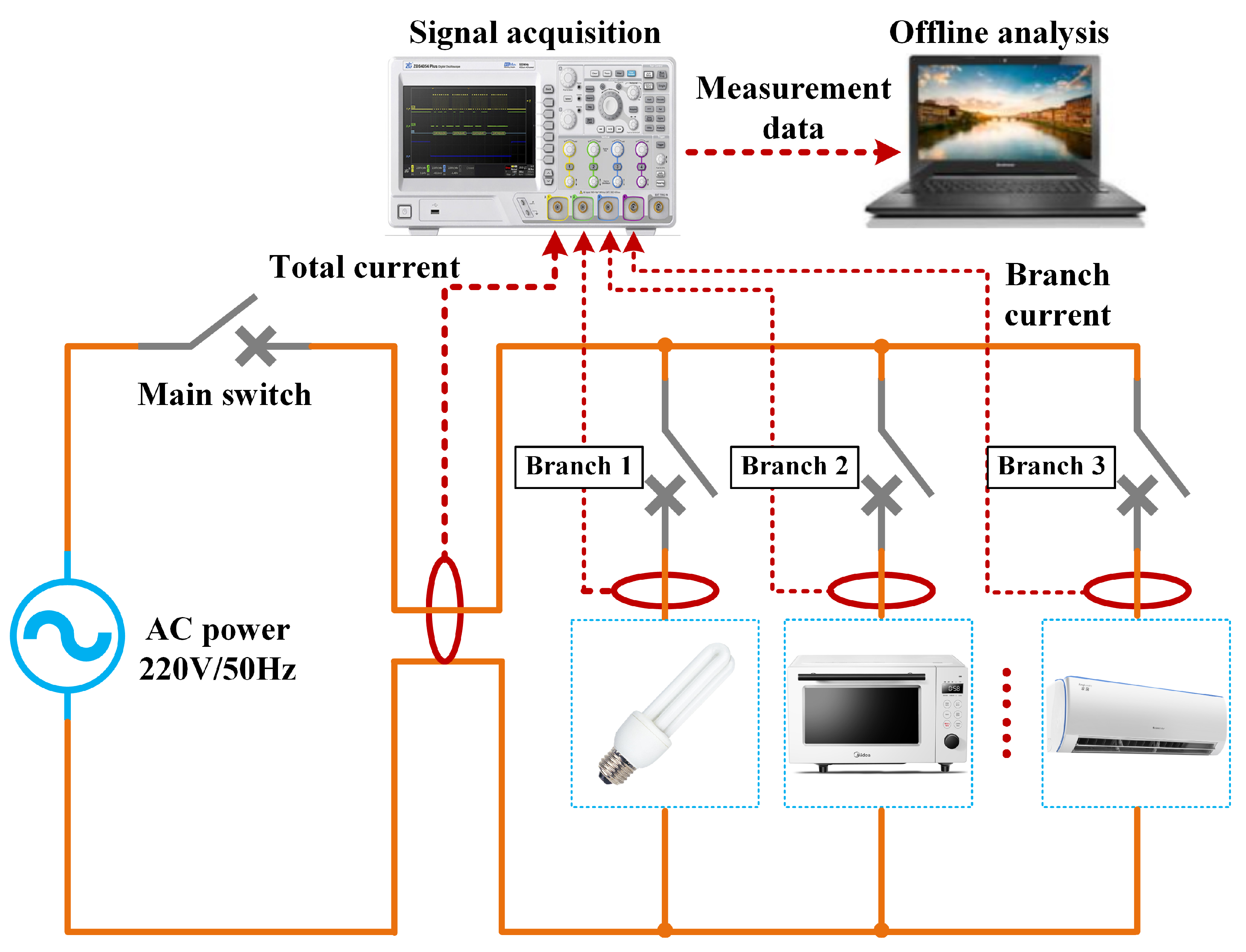
A typical load-stable operation test platform was developed to collect the corresponding laboratory dataset. The operational principles of the platform are illustrated in Figure 1.

The test platform comprises a 220 V/50 Hz single-phase AC power supply, load branch, data acquisition device and other parts, which can realize real-time monitoring and analysis of various power loads. In the laboratory platform, the sampling frequency of each branch signal is configured to be 25 kHz, and the voltage and current signals of the power inlet are simulated by collecting the total loop signal. Due to the limited experimental scenarios and experimental equipment, this paper selects typical electrical loads as data acquisition and analysis objects, including microwave ovens, heaters, incandescent lamps, fluorescent lamps, laptops, vacuum cleaners and hair dryers. These loads cover different load characteristics, such as resistive, inductive, and capacitive and can comprehensively reflect the standard electrical equipment behavior in the home or office environment. In order to study the characteristics of different power loads under stable working conditions, it is necessary to continuously collect current and voltage data for some time after the stable operation of the load to ensure that the data can accurately reflect the steady-state power characteristics and dynamic change trend of the equipment.

2.3. Creation of a Two-Dimensional V–I Trajectory Matrix

Two-dimensional V–I trajectory features are extracted from the voltage and current waveform data of the PLAID dataset, WHITED dataset, and laboratory dataset. The voltage and current waveforms are then mapped to numerical matrices with a specified resolution. For the voltage and current data of a steady-state operation cycle of the load, there are M sampling points (v_m, i_m) in each cycle, where m = 1, 2, … M. The detailed extraction method is outlined as follows:

(1)

Assuming that the size of the V–I trajectory matrix of the mapping is n × n, the normalized voltage and current sampling points are multiplied by n, respectively, and the coordinates of each sampling point in the trajectory matrix (V_m, I_m) can be obtained by taking the downward integer processing, As shown in Equations (1) and (2).

$$V_m=floor(v_{m}n)$$

(1)

$$I_m=floor(i_{m}n)$$

(2)

In the formula, $floor(\cdot )$ represents the downward rounding operation.

(2)

Create an n × n matrix and initialize all elements to 0. For each sampling point, starting from the steady-state period’s initial sampling point, assign a value of 1 to the corresponding i_m row and v_n column elements in the V–I trajectory matrix. Repeat this process for each sampling point until the final one, resulting in the complete V–I trajectory matrix.

The V–I trajectory is a commonly used feature in the field of load identification. However, extracting the trajectory shape parameters is complex, and the choice of characteristic parameters significantly impacts the identification results [32]. Constructing a binary V–I grayscale image can effectively avoid this effect; however, it fails to capture numerical information such as the load’s current, voltage, power, and phase [33,34]. The color V–I image can integrate more detailed feature information of the power load, preserving the shape characteristics of the V–I trajectory while embedding the load’s numerical information into the R, G, and B channels of the color image [35].

2.4. Selection of Load Identification Features

The characteristics used for load identification usually include current, voltage, active power, reactive power, apparent power, and power factor. By analyzing the advantages and disadvantages of each eigenvalue in

Table 2. Comparison of Advantages and Disadvantages of Load Identification Characteristic Values.

Feature	Advantages	Limitations
Voltage and Current	Easy to Measure	Unable to Identify Loads Independently
Active Power	Suitable for Long-Term Monitoring	Different Loads May Have Similar Power Characteristics
Reactive Power	Effective in Distinguishing Resistive Loads	Significant Reactive Power Fluctuations in Electronic Devices
Apparent Power	Reflect the Overall Electrical Characteristics	Cannot Distinguish Loads Individually
Power Factor	Capable of Differentiating Inductive and Resistive Loads	Similar Power Factors Among the Same Type of Loads

, this paper selects instantaneous reactive power, power factor, and load current sequence distribution as key features. Instantaneous reactive power captures load start/stop events and working condition changes, making it ideal for dynamic equipment like motors and air conditioners. Power factor efficiently distinguishes inductive, capacitive, and resistive loads, enabling real-time monitoring. For instance, pure resistive loads (e.g., electric heaters) have a power factor close to 1, while inductive loads (e.g., motors) have lower values. Load current sequence distribution incorporates time dimension information, helping analyze air conditioner frequency changes and refrigerator work cycles.

Based on the above analysis, this paper selects the instantaneous reactive power, power factor and load current sequence distribution as the main features to improve the accuracy of load identification.

2.5. Construction of Mixed-Color Images of Different Loads Based on Harmonic Feature Fusion

The R, G, B pixel matrices with all elements of 0 and size of n × n and three n × 8 order matrices r, g, b are constructed. The instantaneous reactive power is computed using Fryze theory and mapped to the R channel of the color image. Considering the embedded value range of the R channel, the scaling function f(x) = 1/(1 + e^x) is applied, compressing the instantaneous reactive power values to the range (0, 1). The calculation formulas are shown in Equations (3)–(6).

$$P={\displaystyle \frac{1}{M}}{\displaystyle \sum _{m=1}^M{v}_m{i}_m}$$

(3)

$$i_{fm}=i_m-{\displaystyle \frac{P}{V_{\mathrm{rms}}^2}}{v}_m$$

(4)

$$q_m=v_m\cdot i_{fm}$$

(5)

$$R\left(V_m,I_m\right)={\displaystyle \frac{1}{T_m(1+e^{i_{fm}{v}_m})}}$$

(6)

In the formula, P denotes the load’s active power, i_fm represents the load’s reactive current, V_rms is the root mean square value of the periodic voltage, q_m is the instantaneous reactive power, and T_m indicates the number of coordinate points.

The load power factor is selected into the G channel of the color image, where the color depth of the G channel represents the difference in active power among different loads. The formula for calculating the power factor matrix G is shown in Equation (7):

$$G\left(V_m,I_m\right)={\displaystyle \frac{P}{T_m(V_{rms}{I}_{rms})}}$$

(7)

In the formula, I_rms is the root mean square value of the periodic voltage.

The distribution characteristics of the current sequence are selected as the mapping features for the B channel of the color image. The logarithmic function is selected to map the calculated values of the current sequence distribution to the range (0, 1). The calculation formulas for the mapping coordinates corresponding to channel B are shown in Equations (8) and (9).

$$I_e={\displaystyle \frac{1}{M}}{\displaystyle \sum _{m=1}^M{(i_m)}^4}$$

(8)

$$B\left(V_m,I_m\right)={\displaystyle \frac{1}{T_m(1+0.5\lg I_e)}}$$

(9)

In the formula, I_e is the calculated value of current distribution characteristics.

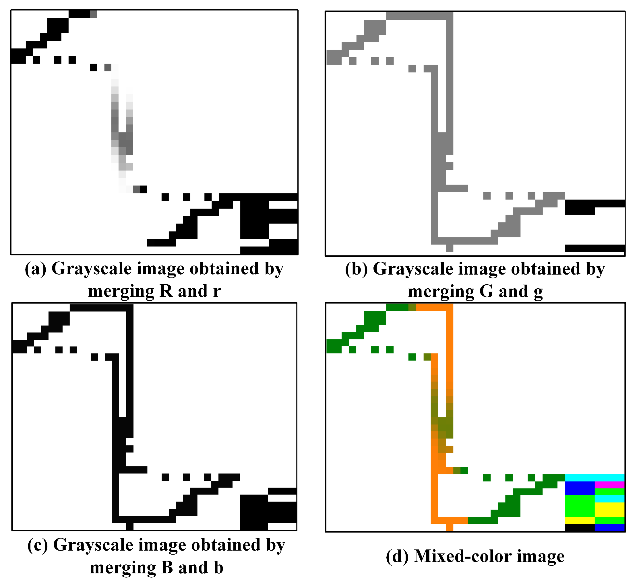
The fundamental frequency amplitude and the third harmonic amplitude of the load current waveform form the first group, the fifth and seventh harmonic amplitudes form the second group, and the ninth and eleventh harmonic amplitudes form the third group. These three sets of harmonic amplitudes are converted into binary values assigned to the first and last four columns of the r, g, and b matrices, respectively. R, G, and B feature matrices are then combined with the r, g, and b matrices to form three hybrid matrices. Using the laptop load as an example, the hybrid color image is constructed following this process, as shown in Figure 2.

Figure 2a shows a gray image representing the V–I trajectory of the laptop, with the color block indicating the magnitude of the fundamental and third harmonic currents. Figure 2b combines the power factor change and the fifth and seventh harmonic amplitudes. Figure 2c reflects the current sequence and the ninth and eleventh harmonic amplitudes. These three grayscale images are combined to form a mixed-color image in Figure 2d, where the color block shows the magnitude of the fundamental wave and five odd harmonics of the laptop’s load current.

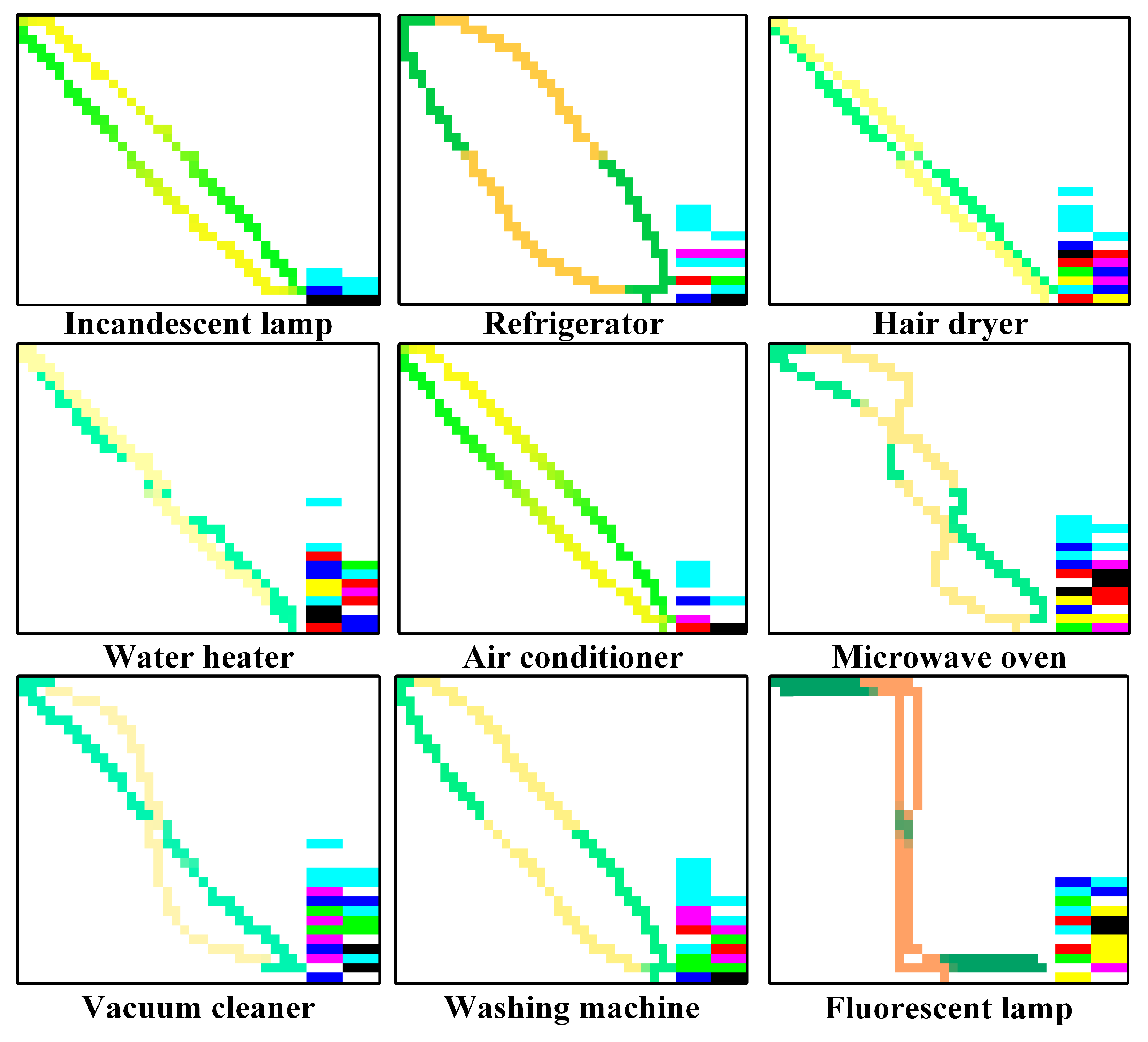
The mixed-color images of the PLAID, WHITED, and laboratory datasets were constructed, respectively. Figure 3 shows the mixed-color images of different types of loads in the PLAID dataset.

It can be seen from Figure 3 that there are significant differences in shape characteristics, color distribution and color change in mixed-color images with different loads, reflecting the power characteristics, transient behavior and current fluctuation mode of various electrical appliances. This visual difference improves the discrimination of the load. Regarding shape, incandescent lamps, hairdryers and heaters are regularly diagonally distributed, while refrigerators, air conditioners and washing machines show arc or curve characteristics. Regarding color distribution, the loads of the same category have certain commonalities, while the colors of fluorescent lamps are significantly different. In terms of color change, the color change in the hair dryer and vacuum cleaner is smooth, while the fluorescent lamp and washing machine show a noticeable color block jump.

Before training the model, the obtained image data are divided into training, validation, and test sets based on a specified proportion. The training set supplies the foundational data for the model to learn. The validation set is used to preliminarily assess the model’s performance and adjust its parameters during training. Finally, the test set evaluates the model’s generalization ability after training is complete.

3. Single-Load Identification Model Based on Atrous Residual Shrinkage Convolutional Network

As shown in the

Table 3. Advantages and Disadvantages of Different Neural Networks.

Network Type	Advantages	Disadvantages	Applicable Scenarios
CNN	Suitable for loading image data.	Not suitable for long time series	Load Mixed-Color Image Classification
RNN	Suitable for time-series modeling	Slow training, prone to gradient vanishing	Load Current Time-Series Analysis
LSTM	Suitable for long-term dependency modeling	Computationally complex, requiring long training times	Load Periodic Feature Extraction

, in load identification, neural networks (such as CNN, RNN, and LSTM) are often used to learn load features to improve the accuracy of classification and recognition. Different types of neural networks have advantages and disadvantages when processing load data. Based on the above table analysis, CNN was selected as the load identification model, considering the computational overhead, model complexity, and actual deployment requirements. CNN has a strong ability in feature extraction and can automatically learn the shape, color distribution and local structure information in the load image while avoiding the tediousness of traditional manual feature engineering. In addition, compared with recurrent neural networks (RNN, LSTM, etc.), CNN can be highly parallelized in the calculation process and has faster training and reasoning speed, which is suitable for real-time load identification tasks. Selecting CNN as the load classification model can reduce the computational overhead and improve the practical application value of the model while ensuring high recognition accuracy.

3.1. The Convolutional Neural Network

A convolutional neural network (CNN) is a powerful network structure in deep learning. The basic structure of a CNN consists of an input layer for data, a convolutional layer for feature extraction, a pooling layer for dimensionality reduction, a Flatten layer, and a fully connected layer [36]. The architecture of a classical CNN is illustrated in Figure 4.

Figure 4 shows the structure of the LeNet-5 classical convolutional neural network (CNN), including the input layer, which is used to receive the input data and preprocess the image. The first convolutional layer extracts low-level features, followed by the first pooling layer, which reduces the data dimension and enhances the model’s robustness. The second convolutional layer extracts higher-level features, and the second pooling layer further reduces the data dimension, improves feature stability, and prevents overfitting. The fully connected convolutional layer extracts global features and provides information for the final classification task. Finally, the first fully connected layer further learns global features and enhances classification capability. The activation function defines the nonlinear mapping relationship between the neuron’s input and output in the above process. In this paper, the ReLU function is selected as the activation function of the CNN network.

3.2. Convolutional Network Based on Dilated Residual Shrinkage

When traditional CNN extracts features from input data, the size of the convolution kernel will limit the ability to extract features. When using large-size convolution kernels, the corresponding receptive field is also larger, and the feature information is more complicated, which greatly increases the computational complexity of the model. Therefore, the convolution kernel size used by CNN is usually small, and the effective feature information of the feature map may be lost during the feature compression process of the pooling layer. The dilated convolution [37] uses the method of doubling convolution to expand the range of the receptive field, which effectively solves the problem that the feature extraction is affected by the convolution kernel size and does not affect the model parameters.

Figure 5 shows the comparison of the receptive field between ordinary convolution and dilated convolution. Different color connections represent different weights corresponding to the convolution kernel. Let the convolution kernel size be 3, and the moving step size be 1, as shown in Figure 5a. At this time, the void rate d = 1, that is, the number of filling weights is 0, and the convolution method of the convolution kernel is ordinary convolution. As shown in Figure 5b, at this time, the hole rate d = 2, the receptive field is 5, and the convolution mode becomes hole convolution, effectively expanding the feature capture range. For loads with similar working principles or low frequency of use in daily life, dilated convolution can extract more subtle features, thereby improving the load identification rate.

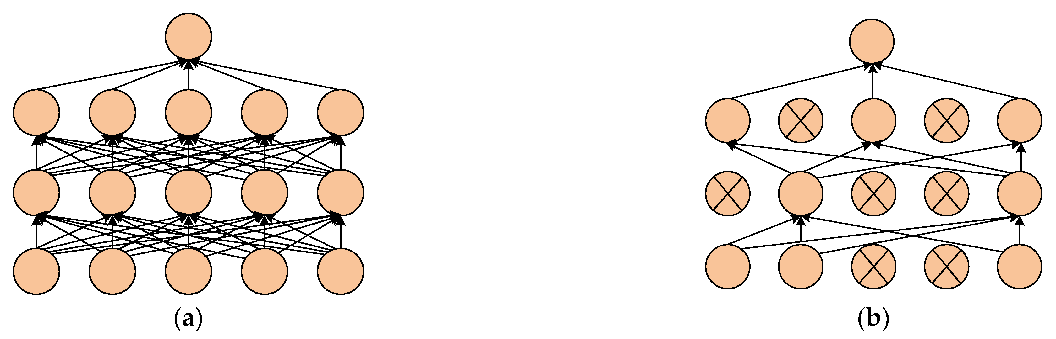
In order to improve the CNN model’s performance, the dropout layer is added to the pooling layer and the fully connected layer.

The main function of the dropout layer is to randomly remove some neurons in the hidden layer according to a certain proportion during the training process and remove the corresponding input and output of the neurons. Figure 6 shows the standard neural network structure and the neural network structure after adding the dropout layer. It can be seen from Figure 6b that the complexity of the network is greatly reduced after adding the dropout layer, which can effectively prevent overfitting.

The feature information extracted by deep neural networks is increasingly rich with the increasing number of network layers and the continuous development of optimization algorithms. However, problems such as gradient disappearance or explosion may occur during the backpropagation process only by superimposing the number of network layers, leading to overfitting or underfitting of the model. To address the poor adaptability of datasets in high-noise environments and enhance image feature extraction, a deep residual shrinkage network is proposed.

The residual shrinkage construction unit serves as the core component of the dilated residual shrinkage network (DRSN). Based on the methods of threshold determination, it can be categorized into channel threshold sharing and channel threshold independence. Given the poor adaptability of datasets in noisy environments and the need to enhance image feature extraction, a deep residual shrinkage network is proposed. The network integrates the residual module, attention mechanism, and soft threshold function. Figure 7 illustrates a schematic diagram of two distinct modules.

The analysis of Figure 7a shows that before the soft threshold operation, the sub-module needs to obtain the absolute value of the output feature map of the upper layer of the network and perform the global average pooling (GAP) operation to obtain the one-dimensional feature vector, and then use the first fully connected layer for batch normalization, and through the activation layer and the second fully connected layer. Among them, the number of neurons in the first fully connected layer equals the number of channels in the feature map C, and the number of neurons in the second fully connected layer is 1. Finally, the sigmoid function is used to map the results to [0, 1], and then the scaling coefficient α of the threshold is obtained, which is multiplied by the average value of x to obtain the channel threshold τ. The difference between the structure shown in Figure 7a and Figure 7b is that the number of neurons in the second fully connected layer in its sub-module is no longer 1 but is consistent with the number of channels in the feature map, that is, the output of the fully connected layer is a one-dimensional vector with the same length and number of channels. After the sigmoid function, each channel’s threshold scaling coefficient α can be obtained, and the threshold corresponding to each channel can be obtained by multiplying it with x.

As shown in the figure above, each channel of the Residual Shrink Building Unit with Channel-Shared Threshold (RSBU-CS) feature map shares a common threshold, and the computational amount of its sub-modules is relatively tiny. However, using the same threshold may result in filtering useful features while retaining noise, affecting the network’s feature extraction performance. Residual Shrink Building Unit with Channel-Wise Threshold (RSBU-CW) has the advantage of adaptively setting the threshold for each channel. The feature extraction capability of different channels is enhanced, improving the model’s performance and aiding its ability to learn the load’s mixed-color features. Therefore, the RSBU-CW module is chosen to build the network model for single-load type identification.

3.3. Model Establishment

A dilated residual shrinkage convolutional network model is constructed using Keras2.3.1 in the Python3.6 programming environment. The model comprises an ordinary convolutional layer and an atrous residual shrinkage module. The ordinary convolutional layer contains 32 convolutional kernels, each with a size of 2 and a stride of 2. The atrous residual shrinkage module consists of a convolutional component and a sub-module. The convolutional module contains two convolution layers. The sub-module comprises a global average pooling layer and two fully connected layers. The model takes a 32 × 40 × 3 mixed-color image dataset as input.

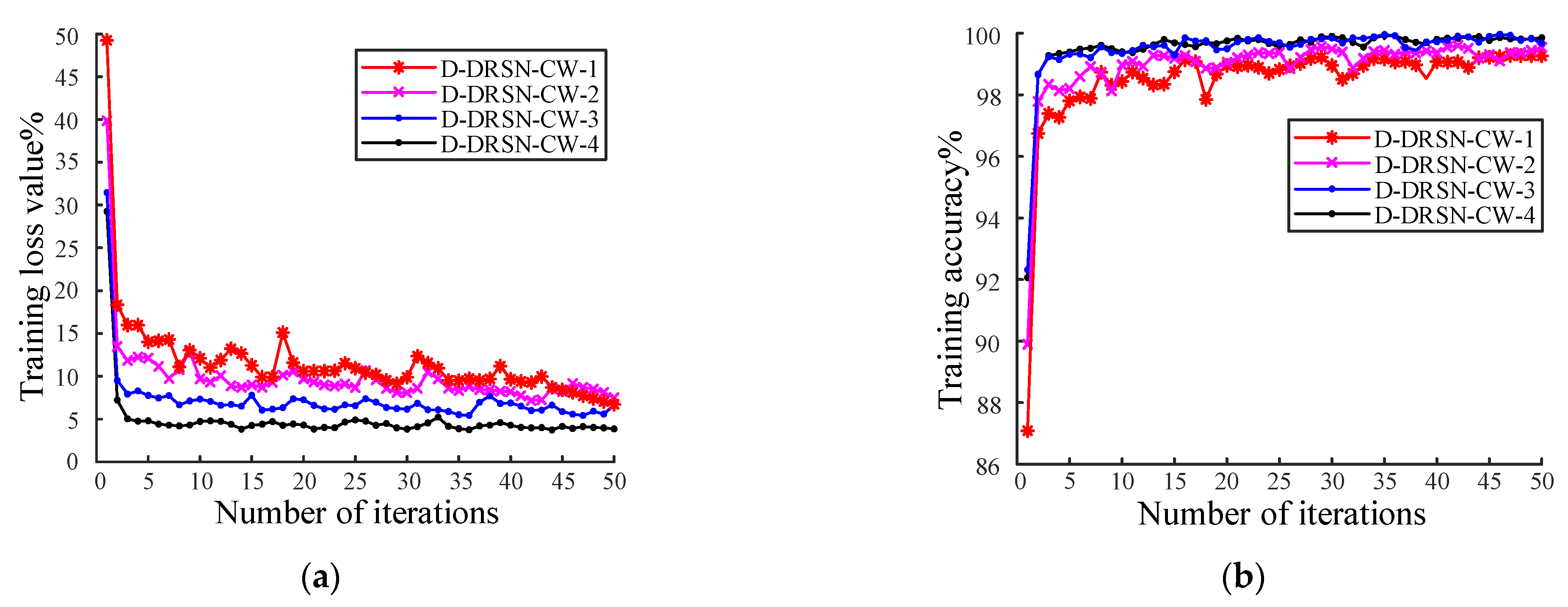
One to four RSBU-CWs are selected to construct the neural network model, with the four models labeled as D-DRSN-CW-n (where n = 1, 2, 3, 4). The parameters of the ordinary convolutional layer are the same across all four models. The convolutional section of the atrous residual shrinkage convolution module contains 30 kernels, with varying atrous rates. The atrous rate of D-DRSN-CW-1 is 1, the atrous rate of D-DRSN-CW-2 is 2, the atrous rate of D-DRSN-CW-3 is 4, and the atrous rate of D-DRSN-CW-4 is 6. The fully connected layer contains 32 neurons, the model is trained for 50 iterations, and the Adam optimizer is used with a batch size of 64. The initial learning rate is set to 0.001. Figure 8 illustrates the model’s training results with varying numbers of atrous residual shrinkage convolution modules. Figure 8a and Figure 8b show the loss values and accuracy curves of the model training process, respectively.

Figure 8 shows that compared with the D-DRSN-CW-1 model, the accuracy of the D-DRSN-CW-2 model is slightly improved, and the final accuracy is about 98.5%. The accuracy of the D-DRSN-CW-3 model exceeds that of the first two models, reaching approximately 99.5%. Simultaneously, during the initial iterations, the accuracy increases more rapidly, while the loss value remains low. This indicates that the network’s learning performance improves as the number of atrous residual modules increases. The accuracy of the D-DRSN-CW-4 model is nearly identical to that of the D-DRSN-CW-3 model, but it has a higher number of parameters. When the atrous rate is too high, the correlation of the convolution results decreases, which may lead to a loss of local information in the image. Considering the number of model parameters and training time, the D-DRSN-CW-3 model is chosen as the model for training with mixed-color images. Based on the above analysis, a single-load identification model using the D-DRSN-CW-3 is built.

4. Analysis of Model Recognition Results

In this section, the results are visually analyzed using a confusion matrix, and the accuracy of this method’s results is compared with the accuracy of ordinary color image recognition. The accuracy of mixed-color image recognition results is higher.

4.1. Analysis of Model Training Results

Figure 9 illustrates the model training process. Panels (a) and (b) of Figure 9 display the change curves of the model’s loss value and accuracy during network iteration.

The diagram above shows that during the first 10 iterations of model training, the loss value of the training set decreased from 0.753 to approximately 0.135, while the accuracy increased from 71.41% to 99.52%. The loss value of the validation set gradually decreased while the accuracy steadily increased. During the 10th to 70th iterations, the loss value of the validation set fluctuated significantly, but the overall trend was downward, while the accuracy remained above 99%. The loss value of the training set decreased steadily, while the accuracy showed a slight increase. By the 70th iteration, the loss value and accuracy of both the training and validation sets stabilized at certain values, indicating that the neural network is nearing convergence. Throughout the iterative process, the change trends of the training and validation sets remained consistent. After all iterations, the accuracy of the training set reached 99.71%, while the accuracy of the validation set was 99.45%.

4.2. Visual Analysis of Recognition Results Based on the Confusion Matrix

To offer a more comprehensive analysis of the identification results across various load types, we use a confusion matrix to visualize the classification outcomes. The PLAID dataset is chosen for this identification process. Figure 10 displays the confusion matrix for the test results of the mixed-color image dataset.

The number indicates the sample count, the black percentage represents the proportion of the current sample count relative to the total, and the red percentage shows the sample recognition error rate. The sum of each column reflects the number of samples used to test the corresponding load in the test set, while the sum of each row indicates the number of samples classified as that load. The numbers in the diagonal blue box represent the number of accurately identified samples in the test set, while those in the yellow box indicate the misclassified samples. The blue percentage in the last column represents the load’s recognition accuracy P_re, while the blue percentage in the last row indicates the load’s recognition recall rate R_re. The calculation formula is presented in Equation (10).

$$\left\{\begin{array}{l}{P}_{\mathrm{re}}={\displaystyle \frac{T_{\mathrm{P}}}{T_{\mathrm{P}}+F_{\mathrm{P}}}}\hfill \\ R_{\mathrm{re}}={\displaystyle \frac{T_{\mathrm{P}}}{T_{\mathrm{P}}+F_{\mathrm{N}}}}\hfill \\ F_{score}={\displaystyle \frac{2P_{\mathrm{re}}{R}_{\mathrm{re}}}{P_{\mathrm{re}}+R_{\mathrm{re}}}}\hfill \end{array}\right.$$

(10)

In the formula, T_P represents the number of instances where the true value is a positive class, and the prediction result is also a positive class; F_P represents the number of instances where the true value is a negative class, and the prediction result is also a negative class; F_N represents the number of instances where the true value is a positive class, and the prediction result is a negative class, and F_score is the harmonic average evaluation index.

For the interpretation of the confusion matrix, as far as the first column of Figure 10 is concerned, there are 383 sets of data in the incandescent lamp, of which 382 sets of data are correctly identified, and only one set of data are mistakenly identified as a washing machine. The recognition accuracy is 99.74%. By analyzing the second column, there are 378 sets of data in the notebook computer, of which 372 sets of data are identified correctly, and only 6 sets of data are mistakenly identified as washing machines, with an accuracy rate of 98.41%. The following sample types are analyzed in the same way.

From the confusion matrix in Figure 10, it can be observed that the model’s average accuracy is approximately 99.56% when using the method proposed in this paper to identify the PLAID dataset. Misjudgments are present in predicting laptops, hair dryers, fluorescent lamps, vacuum cleaners, and washing machines. Among them, the misjudgment rate for washing machines is the highest, with recognition accuracy lower than the average, though it still reaches 98.55%. For loads with similar working principles, such as incandescent lamps, heaters, and hair dryers, color coding creates noticeable differences in the colors within the same graphical area, achieving a recognition accuracy of over 99% For power electronic loads such as notebook current and fluorescent lamp, the recognition accuracy can reach 98%. The above results show that the method is highly accurate and robust in load identification, especially when faced with loads with similar power characteristics and working principles; it can still effectively distinguish.

The method’s generalization ability will be further validated using both the WHITED dataset and a laboratory dataset. The processing process of the WHITED dataset and the laboratory dataset mixed-color image dataset is the same as that of the PLAID dataset. These two datasets add loads from various brand models to verify the model’s generalization ability and improve the accuracy of the generalization test. The test results are shown in

Table 4. Comparison of Accuracy of Different Mixed-Color Image Test Sets.

Load Type	Accuracy
	PLAID Dataset	WHITED Dataset	Laboratory Dataset
Incandescent lamp	100%	99.64%	98.89%
Laptop computer	98.41%	97.23%	99.23%
Hair dryer	99.74%	99.14%	98.87%
Heater	100%	99.74%	97.97%
Fluorescent lamp	99.67%	99.38%	99.30%
Vacuum cleaner	99.21%	97.40%	98.99%
Microwave oven	100%	100%	99.66%
Air conditioner	100%	99.59%	99.11%
Washing machine	98.55%	95.64%	94.46%
Refrigerator	100%	97.62%	96.93%
Average accuracy	99.56%	98.54%	98.34%

.

Table 4 shows the test results of the WHITED and laboratory datasets. However, the recognition accuracy of various loads has decreased, and the average accuracy rate is still above 98.34%. The data acquisition method used in the laboratory dataset is oscilloscope acquisition. There is an inherent error of 2%, which may be one of the reasons for the decrease in recognition results and also one of the directions for subsequent improvement. Overall, although the test accuracy in the WHITED and laboratory datasets has declined, the overall accuracy remains high, demonstrating that the proposed method maintains good recognition performance across different data environments. In particular, its classification performance is more pronounced for loads with stable characteristics. This further indicates that the proposed method has significant practical value in intelligent power systems, energy consumption monitoring, and appliance state identification applications.

5. Discussion

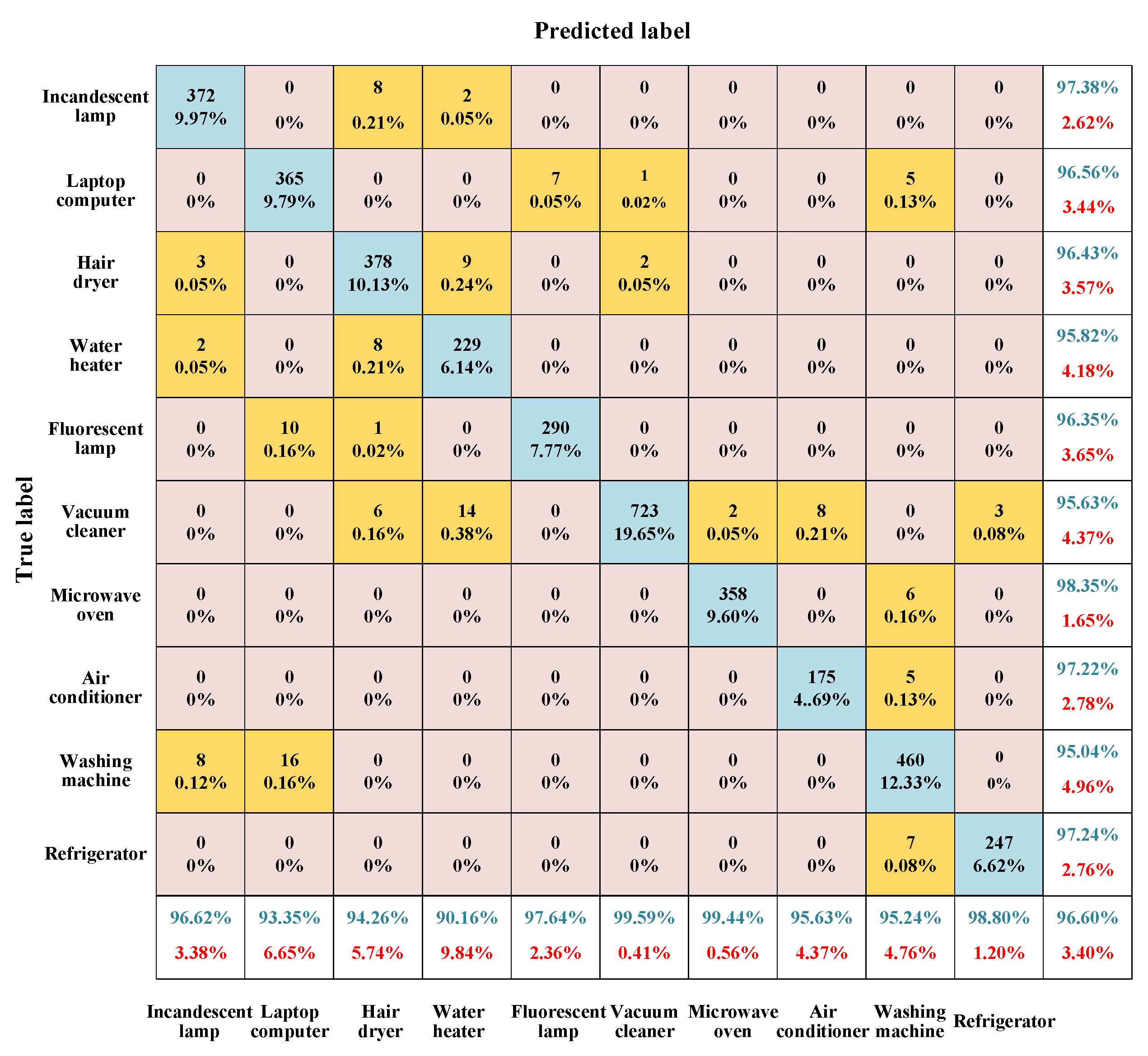
In order to further verify the advantages of the hybrid color image proposed in this paper for load identification, this section compares the recognition accuracy with that of ordinary color images. Based on the PLAID dataset, WHITED dataset, and laboratory dataset, an ordinary color image dataset is constructed. The construction steps for ordinary color images are the same as those for mixed-color images, with the only difference being that the V–I trajectory is mapped to the RGB color space, and the voltage, current, and time are mapped to the R, G, and B channels, respectively. The other network parameter settings are the same as those for the mixed-color image recognition model. The confusion matrix of the test results for the standard color image dataset based on the PLAID dataset is shown in Figure 11.

Figure 11 shows that the average accuracy of ordinary color images is 96.60%. Compared with the hybrid color image method used in this paper, the accuracy is reduced by 2.96%. The results show that this paper’s hybrid color image method performs better in the load recognition task and can effectively improve recognition accuracy.

In addition,

Table 5. Comparison of Accuracy of Different Ordinary Color Image Test Sets.

Load Type	Accuracy
	PLAID Dataset	WHITED Dataset	Laboratory Dataset
Incandescent lamp	97.38%	95.37%	92.48%
Laptop computer	96.56%	95.09%	94.21%
Hair dryer	96.43%	92.70%	90.40%
Heater	95.81%	94.31%	91.86%
Fluorescent lamp	96.35%	97.05%	95.30%
Vacuum cleaner	95.63%	95.05%	95.21%
Microwave oven	98.35%	96.52%	95.93%
Air conditioner	97.22%	96.83%	96.44%
Washing machine	95.04%	94.31%	93.66%
Refrigerator	97.24%	92.70%	92.33%
Average accuracy	96.60%	94.99%	93.78%

shows the load recognition accuracy test results of the three datasets after using the standard color image construction method. Compared with the method proposed in this paper, the recognition accuracy of ordinary color images is reduced. Among them, the test accuracy of the WHITED dataset was reduced by 1.61%, while the test accuracy of the laboratory dataset was reduced by 2.82%. This trend further verifies the effectiveness of the hybrid color image method, indicating that the method can extract the load characteristics more accurately and improve the recognition performance.

To further verify the proposed method’s performance, three existing load feature extraction methods, classification models, and recognition accuracy are compared [38,39,40]. The results are shown in

Table 6. Comparison of Recognition Results from Different Literature Methods.

Model	Feature Extraction	Accuracy
MLP [38]	Harmonic current	73.0%
BP + LeNet-5 [39]	V–I trajectory, power features	90.9%
CNN [40]	V–I trajectory, power, higher-order harmonics	93.2%
The D-DRSN model proposed in this paper.	Mixed-color image	99.56%

. Regarding model recognition ability, load recognition based on D-DRSN is significantly better than that of CNN alone. Compared with LeNet-5 and BP neural networks [39], D-DRSN maintains a higher recognition accuracy, while the model complexity and calculation efficiency are lower. Regarding load feature extraction, this method combines harmonic features and color V–I trajectory images, covers all the features used in the literature [40], and introduces new load features. Therefore, the proposed method can characterize load characteristics more comprehensively.

The experimental results show that this method’s recognition accuracy is 26.26%, 8.66% and 6.36% higher than that of the other three methods, respectively. This method effectively reduces the misjudgment rate, especially in the identification of multi-state operating loads and similar working principles, further verifying its robustness and applicability.

6. Conclusions

This paper employs color coding technology to map the instantaneous reactive power, power factor, and current sequence distribution eigenvalues of the load to the R, G, and B channels of a color image. By integrating current harmonic characteristics, a mixed-load color image dataset is established. The characteristics, advantages, and disadvantages of two residual shrinkage units, RSBU-CS and RSBU-CW, are compared and analyzed. Based on this analysis, a single-load identification model incorporating three RSBU-CW modules is developed. The performance of the model is validated by different datasets. The test results demonstrate that the model accurately identifies the load. The model achieves an accuracy of 99.56% on the PLAID dataset, 98.54% on the WHITED dataset, and 98.34% on the laboratory dataset. The ordinary color image is constructed and compared with the mixed-color image method. The results show that the mixed-color image method has higher recognition accuracy. Accurate load identification plays a crucial role in enhancing the safety and stability of power systems. By improving the accuracy of load recognition, the proposed method facilitates real-time monitoring, fault detection, and optimized energy management, contributing to the reliability and efficiency of modern smart grids.

The method proposed in this paper has the advantage that the complexity of the model used is lower than that of the general network model, but the recognition accuracy is higher. At the same time, the results of the verification of multi-source data show that the method has strong robustness. Although this method has achieved high recognition accuracy in load classification, some limitations remain. First, although the complexity of the model is lower than that of some neural networks, the computational resource consumption is still high, which may not be suitable for embedded devices or real-time applications. It should be noted that the load types and brands identified in this study are limited, whereas real-world industrial and residential settings involve a wider variety of electrical loads. Therefore, the scope of identifiable load types should be expanded. Moreover, the data used in this study are exclusively obtained from low-voltage household appliances. As such, the applicability of the proposed load identification method to medium- and high-voltage domains requires further investigation and validation.

Future research directions can consider the following aspects: (1) further optimize the network structure, such as combining an attention mechanism or a lightweight neural network to improve computational efficiency; (2) introduce more abundant load characteristics, such as timing dynamic information, to improve the ability to distinguish complex loads; (3) research data augmentation strategy to improve the model’s adaptability to different load environments.