Calculations of Electrical Parameters of Cables in Wide Frequency Range

Abstract

The significant capacitive effects of cables can cause resonance stability issues, making it crucial to accurately model cables in the wide frequency range (up to several kilo-Hertz) where resonance typically occurs. To address the complexity and the neglect of cable bonding and earthing arrangements in previous accurate cable modeling, this paper derives a concise analytical method for calculating cable electrical parameters over the wide frequency range, simplifying the prior complex formulas, clarifying the series impedance components, and comprehensively considering three common bonding and earthing arrangements. The case studies of three-core and single-core submarine cables are presented to verify the effectiveness of the improved analytical method. The analysis includes frequency-dependent per-unit-length parameters and the impact of each component on the series impedances. Furthermore, a simplified algorithm is explored, avoiding Bessel function computations based on the impedance component impact study, as well as infinite series calculations by considering the effect of the earth/sea return path position factor on the simplified series accuracy.

1. Introduction

Cables are crucial components in the transmission and distribution stages of power systems. On the one hand, underground cables are widely used in urban power systems due to their small footprint and high reliability in power supply [1]. On the other hand, submarine cables are used for power transmission between islands and the mainland, and their usage is expected to grow with the boost of offshore wind power [2,3].

However, cables have significant capacitive effects, which will lead to resonance stability issues if not properly coordinated with the inductive components in the system [4,5]. For resonance stability analysis in large power systems, modal analysis is commonly used, where each component is represented by an impedance model [6,7]. Ref. [8] models cables by considering only distribution effects and neglecting frequency-dependent effects, leading to significant errors. Therefore, for the frequency-dependent factors, Ref. [9] only considers the conductors’ skin effect, which improves the cable model’s accuracy but is still insufficient. For resonance stability analysis, it is crucial to accurately model cables with complex structures in the wide frequency range (within 2 kHz [10]) where resonance typically occurs.

Cable electrical parameters can be calculated by either the analytical or the numerical method.

The analytical method is simple to operate and relatively efficient. The impedance of the earth return path derived in [11,12], along with the AC impedances of cylindrical conductors derived in [13], forms the foundation. In [14,15], the series impedance and shunt admittance matrices for cables are established, but the effects of bonding and earthing arrangements are neglected with the use of complex formulas. The power-frequency cable formulas were derived in [16], but wide-frequency ones were not provided, despite more concise wide-frequency formulas being offered for overhead line modeling. Ref. [17] applies vector fitting to calculate the frequency-dependent conductor impedances, equivalent to solving Foster network parameters. In summary, the existing analytical methods have the following issues: complex formulas involving Bessel functions and infinite series, neglect of bonding and earthing arrangements, and lack of study on the impact of each component on series impedances.

The numerical method, which mainly includes the finite element method and the subdivided conductor method, provides comprehensive analysis and high accuracy. In [18,19,20], the finite element method was first used for cable parameter calculations, but neglecting displacement current in the earth/sea return path based on a quasistatic electric field can cause errors at high frequencies. Ref. [21] overcame the limitation of quasistatic electric fields by using the finite element method for modal analysis and stated that displacement currents can be neglected below 10 kHz. In [22], the subdivided conductor method is used to account for the conductor proximity effect, with a comparison of results for circular, square, and arc subdivisions. Ref. [23] also uses the subdivided conductor method and considers the effect of horizontally stratified soil, noting that the proximity effect can be neglected below 10 kHz. Overall, the numerical method is inefficient, and its advantage over analytical methods in accounting for the displacement current and proximity effect is not significant in the concerned frequency range of this paper (up to several kilo-Hertz).

To this end, this paper derives a concise analytical method for calculating cable electrical parameters over the wide frequency range, considering the effects of cable bonding and earthing arrangements based on the wide-frequency formulas for overhead lines [16]. Furthermore, this paper explores a simplified algorithm, avoiding Bessel function computations based on the impedance component impact study, as well as infinite series calculations by considering the effect of the earth/sea return path position factor on the simplified series accuracy.

The rest of this paper includes four parts. In Section 2, the structures, bonding, earthing arrangements, and layouts of the cables are introduced, providing a foundation for the subsequent electrical parameter computations. In Section 3, a concise analytical method for calculating cable electrical parameters is derived, covering geometric parameters preprocessing, construction of full electrical parameter matrices, and transformation to sequence electrical parameter matrices based on bonding and earthing arrangements. In Section 4, the case studies of three-core and single-core submarine cables are presented to demonstrate the effectiveness of the improved analytical method; it also analyzes the frequency-dependent per-unit-length parameters, studies the impact of various components on series impedances, and explores a simplified algorithm. The conclusions are summarized in Section 5.

2. Structures and Arrangements of Cables

2.1. Structures of Cables

A cable consists of multiple coaxial conductors and insulations. The conductors, from inner to outer, include the core, sheath, and armor (not all cables have all three). Insulations are placed between adjacent conductors. Based on the number of cores, cables can be classified as single-core or three-core.

This paper demonstrates the calculations of electrical parameters by two of the most complex cables: a single-core and a three-core cable, both with armor, whose simplified structures are shown in Figure 1.

In Figure 1, the subscript i of each parameter is the phase identifier, where i = A, B, C, 0 (0 specifically refers to the phase of the three-core cable’s armor, used for analysis convenience even though the armor does not belong to any phase); the subscripts c, s, a, and E correspond to the core, sheath, armor, and earth/sea, respectively; r_{i_ic} and r_{o_ic} are the inner and outer radii of the core; r_{i_is} and r_{o_is} are the inner and outer radii of the sheath; r_{i_ia} and r_{o_ia} are the inner and outer radii of the armor; t_ips is the thickness of the armor insulation; ε_ics, ε_isa, and ε_iaE are the relative permittivities of the core, sheath, and armor insulation, respectively. The structural parameters are the same for all phases.

2.2. Bonding and Earthing Arrangements of Cables

The sheaths serve multiple functions, including isolating moisture, providing a return path for short-circuit fault current, and protecting against mechanical damage. To limit the voltages on the sheaths induced by the currents in the cores, various bonding and earthing methods are employed. Three common methods are introduced below [16].

First, the solid bonding method. Both ends of the three-phase cables’ sheaths are connected and directly earthed, as shown in Figure 2. Under the zero-sequence voltage, the sheaths provide a return path for the short-circuit fault current. However, under the positive sequence voltage, the induced currents can generate heat and potentially damage the cables.

Second, the single-point bonding method. This method can be further divided into three variations. For the shorter cables, one end of the three-phase cables’ sheaths is connected and directly earthed, while the other is grounded through voltage limiters (Figure 3a), limiting the induced voltages and preventing current circulation during normal operation. For the longer cables, both ends are earthed through voltage limiters, with the midpoint connected and directly grounded (Figure 3b). In practice, an extra conductor, grounded at both ends and transposed, is applied to provide a path for currents under the zero-sequence earth fault while carrying no current during normal operation (Figure 3c).

Third, the cross-bonding method. This method is typically applied for longer cables. The three-phase cables are divided into multiple cross-bonding groups, each consisting of three equal-length sections, as plotted in Figure 4. Both ends of the group are directly earthed, while the middle section is grounded through voltage limiters, which eliminates the need for an extra conductor as in the single-point bonding method. The cores are transposed perfectly, but the other conductors are not. During normal operation, the induced voltages across each section cancel out, resulting in zero total voltage and no induced current.

Additionally, to control the voltages between the sheaths and armors, they are usually connected at multiple points along the cables, making their grounding identical.

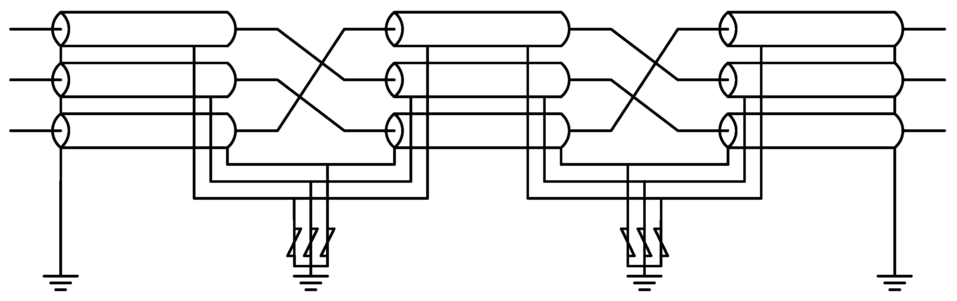
2.3. Layouts of Cables

Typical cable layouts include flat, triangular, and their variants, as shown in Figure 5. Symmetrical layouts can simplify the calculations of electrical parameters.

3. Calculations of Electrical Parameters of Cables

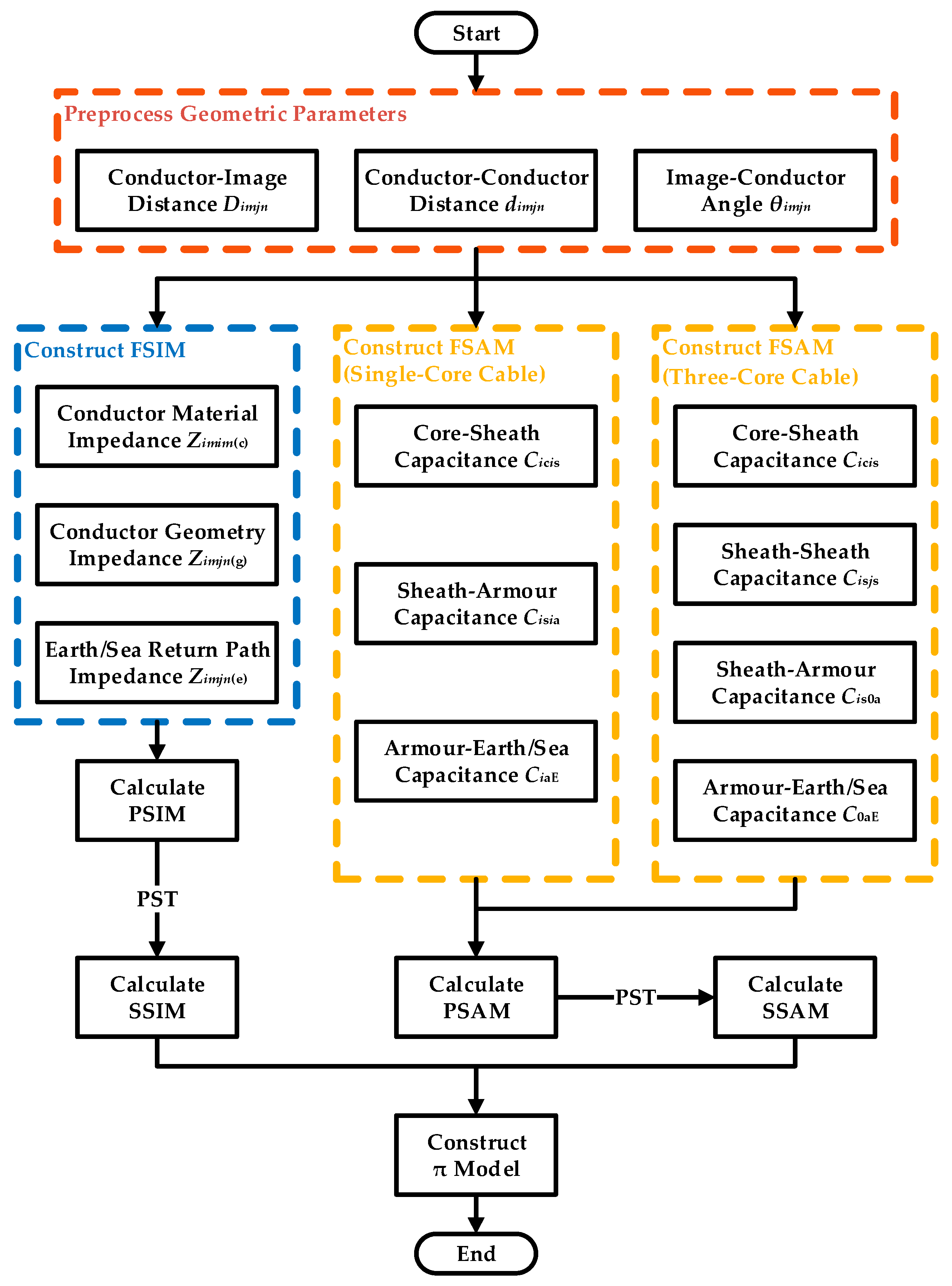
3.1. Process Overview

In resonance stability analysis, cables are typically represented by the π models (Figure 6) that consider the characteristic of the parameter’s even distribution. In Figure 6, Z_cable and Y_cable are the series impedance and shunt admittance of the entire cable, calculated as follows [24]:

$$Z_{\mathrm{cable}}=Z_{\mathrm{c}}\sinh \left(\gamma L\right)={\displaystyle \frac{\sinh \left(\gamma L\right)}{\gamma L}}zL=K_{Z}zL$$

(1)

$$Y_{\mathrm{cable}}={\displaystyle \frac{\cosh \left(\gamma L\right)-1}{Z_{\mathrm{c}}\sinh \left(\gamma L\right)}}={\displaystyle \frac{\tanh \left(\gamma L/2\right)}{\gamma L/2}}{\displaystyle \frac{yL}{2}}=K_Y{\displaystyle \frac{yL}{2}}$$

(2)

$$Z_{\mathrm{c}}=\sqrt{z/y}$$

(3)

$$\gamma =\sqrt{zy}$$

(4)

where L is the cable length; Z_c is the characteristic impedance; γ is the propagation constant; z and y are the per-unit-length series impedance and shunt admittance for each sequence, respectively; K_Z and K_Y are the correction factors for the series impedance and shunt admittance, respectively.

To establish the π model, z and y are derived from the cables’ geometric parameters, whose process is illustrated in Figure 7. Firstly, the cables’ geometric parameters, including structural and positional ones, are preprocessed to obtain three parameters for the full electrical parameter matrices, as introduced in Section 3.2. Next, construct the full series impedance matrix (FSIM) and full shunt admittance matrix (FSAM). The FSIM elements consist of three impedance components from conductor material, conductor geometry, and earth/sea return path, with their computations shown in Section 3.3. Ignoring shunt conductances, the calculation of the capacitances between conductors forming the FSAM elements is presented in Section 3.5. Then, based on the cables’ bonding and earthing arrangements, convert the FSIM and FSCM into the phase series impedance matrix (PSIM) and phase shunt admittance matrix (PSAM). Finally, apply phase-sequence transformation (PST) to convert the PSIM and PSAM into the sequence series impedance matrix (SSIM) and sequence shunt admittance matrix (SSAM), with the diagonal elements as z and y. The above two processes are discussed in Section 3.4 and Section 3.6, respectively.

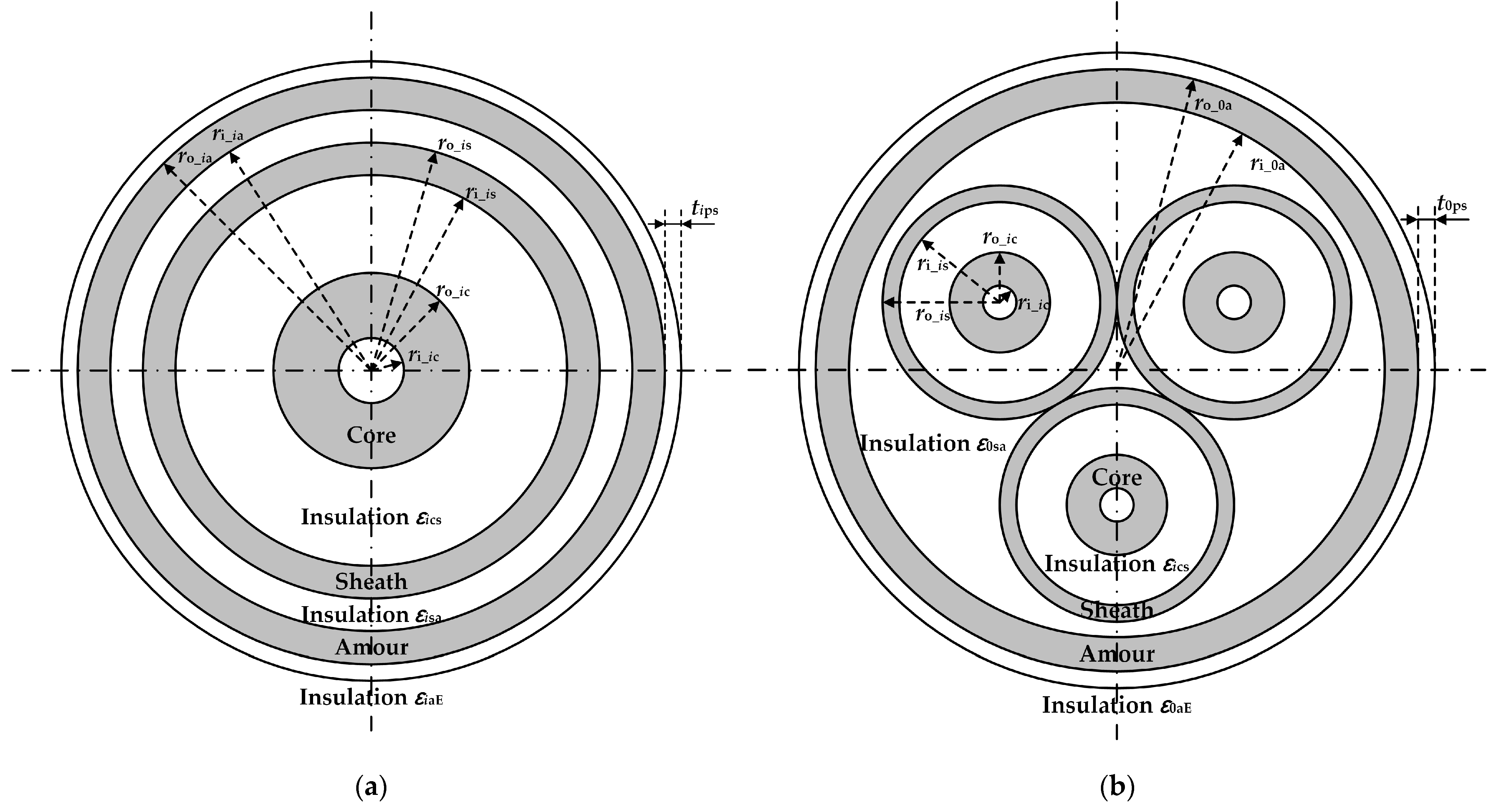
3.2. Geometric Parameters Preprocessing

The FSIM is constructed by the method of images. The cables and their images are shown in Figure 8. The earth/sea surface is typically chosen as the horizontal axis, with the conductors’ vertical coordinates positive and the images’ negative. The vertical axis can be arbitrarily selected. To apply the image method, the cables’ structural and positional parameters need to be preprocessed to obtain the following parameters.

x_i and y_i represent the average horizontal and vertical coordinates of the axis of the conductor in phase i, calculated as follows:

$$\left\{\begin{array}{l}{x}_i=\left[{\displaystyle {\int }_0^L{x}_{i0}\left(l\right)\mathrm{d}l}\right]/L\hfill \\ y_i=\left[{\displaystyle {\int }_0^L{y}_{i0}\left(l\right)\mathrm{d}l}\right]/L\hfill \end{array}\right.$$

(5)

where x_i0 and y_i0 are the original horizontal and vertical coordinates of the axis of the conductor in phase i, which are the functions of cable length l. Furthermore, the corresponding image’s coordinates satisfy x_i = x_i′ and y_i′ = −y_i.

D_imjn represents the distance between the axis of conductor m in phase i and the axis of the image of conductor n in phase j.

For single-core cables, D_imjn is calculated as follows:

$$D_{imjn}=\sqrt{{\left(x_i-{x_j}^{\prime }\right)}^2+{\left(y_i-{y_j}^{\prime }\right)}^2}$$

(6)

For a three-core cable, since the axes of the conductors are very close to each other, the armor’s axis can replace others in the calculation of the positional parameters involving images. D_imjn is calculated as follows:

$$D_{imjn}\approx 2y_0$$

(7)

d_imjn represents the distance between conductor m’s axis in phase i and conductor n’s axis in phase j, or the conductor’s outer radius.

For single-core cables, d_imjn is calculated as follows:

$$d_{imjn}=\left\{\begin{array}{l}\sqrt{{\left(x_i-x_j\right)}^2+{\left(y_i-y_j\right)}^2}\hspace{1em}i\ne j\hfill \\ r_{\mathrm{o}\_jn}\hspace{1em}i=j, m\subset n\hfill \\ r_{\mathrm{o}\_im}\hspace{1em}i=j, m\supset n\hfill \\ r_{\mathrm{o}\_im}\hspace{1em}i=j, m=n\hfill \end{array}\right.$$

(8)

where case 1 refers to conductors m and n being on different axes, and the other cases refer to conductors m and n being coaxial, with case 2 referring to conductor n being the outer conductor, case 3 referring to conductor m being the outer conductor, and case 4 referring to conductors m and n being the same conductor.

In the case where one conductor contains another, regardless of whether the two conductors are coaxial, d_imjn is the outer radius of the outer conductor. For a three-core cable, d_0aim and d_im0a, involving the armor that surrounds the other conductors, are calculated as follows:

$$d_{0\mathrm{a}im}=d_{im0\mathrm{a}}=r_{\mathrm{o}\_0\mathrm{a}}$$

(9)

For d_imjn not involving the armor, (8) still applies.

θ_imjn represents the angle between the line connecting the axes of conductor m and its image in phase i, and the line connecting the axis of conductor m in phase i to the axis of conductor n’s image in phase j.

For single-core cables, θ_imjn is calculated as follows:

$${\theta }_{imjn}={\cos }^{-1}\left({\displaystyle \frac{y_i+y_j}{D_{imjn}}}\right)$$

(10)

For a three-core cable, θ_imjn is calculated as follows:

$${\theta }_{imjn}\approx 0$$

(11)

For touching triangular layout single-core cables, since the cable axes are very close, the positional parameters associated with the images can be calculated with the layout center instead of the axes. Thus, their geometric parameters preprocessing is similar to that of a three-core cable and will not be repeated here.

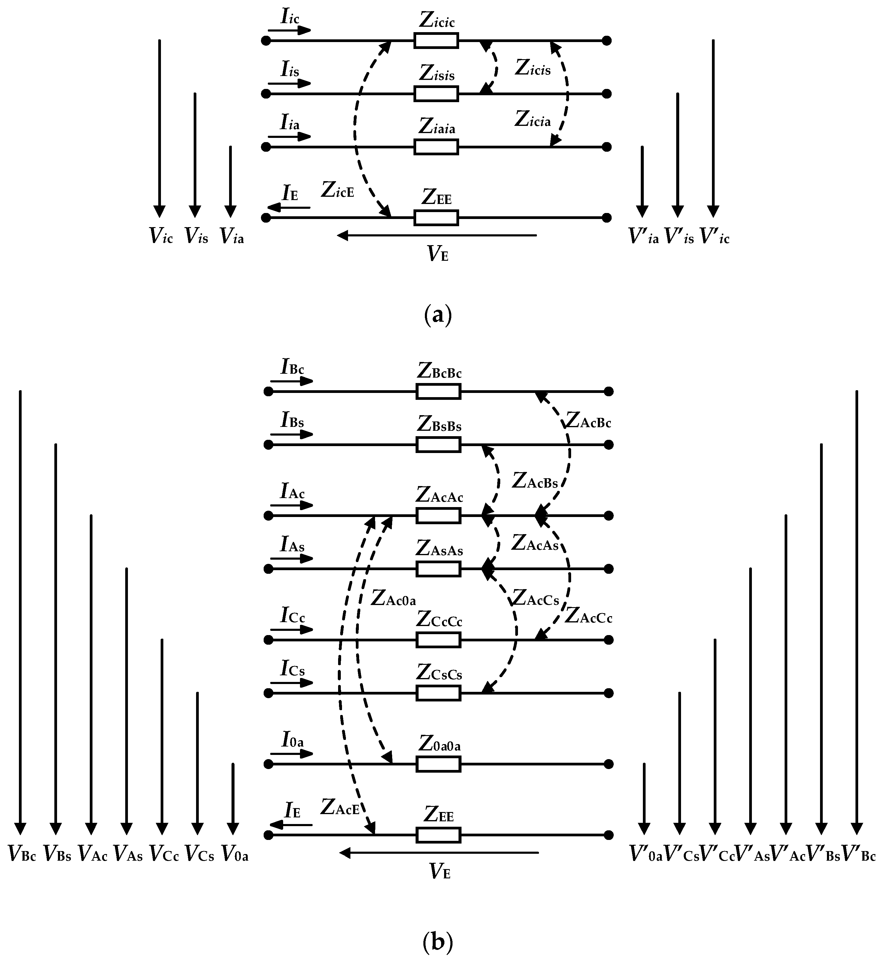
3.3. Construction of FSIM

The series voltage equations for single-core and three-core cables are listed as follows [15], with their detailed derivations provided in Appendix A. In the equation, Z_Full is the FSIM, with elements Z_imjn-E. The subscripts i and j are the phase identifiers (i, j = A, B, C, 0), m and n are the conductor identifiers (m, n = c, s, a), and E indicates that the impedance includes the effect of the earth/sea return path.

$$\begin{array}{l}\left[\begin{array}{c}\Delta V_{\mathrm{Ac}}\\ \Delta V_{\mathrm{Bc}}\\ \Delta V_{\mathrm{Cc}}\\ \Delta V_{\mathrm{As}}\\ \Delta V_{\mathrm{Bs}}\\ \Delta V_{\mathrm{Cs}}\\ \Delta V_{\mathrm{Aa}}\\ \Delta V_{\mathrm{Ba}}\\ \Delta V_{\mathrm{Ca}}\end{array}\right]=\left[\begin{array}{ccccccccc}{Z}_{\mathrm{AcAc}\text{-}\mathrm{E}}& Z_{\mathrm{AcBc}\text{-}\mathrm{E}}& Z_{\mathrm{AcCc}\text{-}\mathrm{E}}& Z_{\mathrm{AcAs}\text{-}\mathrm{E}}& Z_{\mathrm{AcBs}\text{-}\mathrm{E}}& Z_{\mathrm{AcCs}\text{-}\mathrm{E}}& Z_{\mathrm{AcAa}\text{-}\mathrm{E}}& Z_{\mathrm{AcBa}\text{-}\mathrm{E}}& Z_{\mathrm{AcCa}\text{-}\mathrm{E}}\\ Z_{\mathrm{BcAc}\text{-}\mathrm{E}}& Z_{\mathrm{BcBc}\text{-}\mathrm{E}}& Z_{\mathrm{BcCc}\text{-}\mathrm{E}}& Z_{\mathrm{BcAs}\text{-}\mathrm{E}}& Z_{\mathrm{BcBs}\text{-}\mathrm{E}}& Z_{\mathrm{BcCs}\text{-}\mathrm{E}}& Z_{\mathrm{BcAa}\text{-}\mathrm{E}}& Z_{\mathrm{BcBa}\text{-}\mathrm{E}}& Z_{\mathrm{BcCa}\text{-}\mathrm{E}}\\ Z_{\mathrm{CcAc}\text{-}\mathrm{E}}& Z_{\mathrm{CcBc}\text{-}\mathrm{E}}& Z_{\mathrm{CcCc}\text{-}\mathrm{E}}& Z_{\mathrm{CcAs}\text{-}\mathrm{E}}& Z_{\mathrm{CcBs}\text{-}\mathrm{E}}& Z_{\mathrm{CcCs}\text{-}\mathrm{E}}& Z_{\mathrm{CcAa}\text{-}\mathrm{E}}& Z_{\mathrm{CcBa}\text{-}\mathrm{E}}& Z_{\mathrm{CcCa}\text{-}\mathrm{E}}\\ Z_{\mathrm{AsAc}\text{-}\mathrm{E}}& Z_{\mathrm{AsBc}\text{-}\mathrm{E}}& Z_{\mathrm{AsCc}\text{-}\mathrm{E}}& Z_{\mathrm{AsAs}\text{-}\mathrm{E}}& Z_{\mathrm{AsBs}\text{-}\mathrm{E}}& Z_{\mathrm{AsCs}\text{-}\mathrm{E}}& Z_{\mathrm{AsAa}\text{-}\mathrm{E}}& Z_{\mathrm{AsBa}\text{-}\mathrm{E}}& Z_{\mathrm{AsCa}\text{-}\mathrm{E}}\\ Z_{\mathrm{BsAc}\text{-}\mathrm{E}}& Z_{\mathrm{BsBc}\text{-}\mathrm{E}}& Z_{\mathrm{BsCc}\text{-}\mathrm{E}}& Z_{\mathrm{BsAs}\text{-}\mathrm{E}}& Z_{\mathrm{BsBs}\text{-}\mathrm{E}}& Z_{\mathrm{BsCs}\text{-}\mathrm{E}}& Z_{\mathrm{BsAa}\text{-}\mathrm{E}}& Z_{\mathrm{BsBa}\text{-}\mathrm{E}}& Z_{\mathrm{BsCa}\text{-}\mathrm{E}}\\ Z_{\mathrm{CsAc}\text{-}\mathrm{E}}& Z_{\mathrm{CsBc}\text{-}\mathrm{E}}& Z_{\mathrm{CsC}\mathrm{c}\text{-}\mathrm{E}}& Z_{\mathrm{CsAs}\text{-}\mathrm{E}}& Z_{\mathrm{CsBs}\text{-}\mathrm{E}}& Z_{\mathrm{CsC}\mathrm{s}\text{-}\mathrm{E}}& Z_{\mathrm{CsAa}\text{-}\mathrm{E}}& Z_{\mathrm{CsBa}\text{-}\mathrm{E}}& Z_{\mathrm{CsC}\mathrm{a}\text{-}\mathrm{E}}\\ Z_{\mathrm{AaAc}\text{-}\mathrm{E}}& Z_{\mathrm{AaBc}\text{-}\mathrm{E}}& Z_{\mathrm{AaCc}\text{-}\mathrm{E}}& Z_{\mathrm{AaAs}\text{-}\mathrm{E}}& Z_{\mathrm{AaBs}\text{-}\mathrm{E}}& Z_{\mathrm{AaCs}\text{-}\mathrm{E}}& Z_{\mathrm{AaAa}\text{-}\mathrm{E}}& Z_{\mathrm{AaBa}\text{-}\mathrm{E}}& Z_{\mathrm{AaCa}\text{-}\mathrm{E}}\\ Z_{\mathrm{BaAc}\text{-}\mathrm{E}}& Z_{\mathrm{BaBc}\text{-}\mathrm{E}}& Z_{\mathrm{BaCc}\text{-}\mathrm{E}}& Z_{\mathrm{BaAs}\text{-}\mathrm{E}}& Z_{\mathrm{BaBs}\text{-}\mathrm{E}}& Z_{\mathrm{BaCs}\text{-}\mathrm{E}}& Z_{\mathrm{BaAa}\text{-}\mathrm{E}}& Z_{\mathrm{BaBa}\text{-}\mathrm{E}}& Z_{\mathrm{BaCa}\text{-}\mathrm{E}}\\ Z_{\mathrm{CaAc}\text{-}\mathrm{E}}& Z_{\mathrm{CaBc}\text{-}\mathrm{E}}& Z_{\mathrm{CaCc}\text{-}\mathrm{E}}& Z_{\mathrm{CaAs}\text{-}\mathrm{E}}& Z_{\mathrm{CaBs}\text{-}\mathrm{E}}& Z_{\mathrm{CaCs}\text{-}\mathrm{E}}& Z_{\mathrm{CaAa}\text{-}\mathrm{E}}& Z_{\mathrm{CaBa}\text{-}\mathrm{E}}& Z_{\mathrm{CaCa}\text{-}\mathrm{E}}\end{array}\right]\left[\begin{array}{c}{I}_{\mathrm{Ac}}\\ I_{\mathrm{Bc}}\\ I_{\mathrm{Cc}}\\ I_{\mathrm{As}}\\ I_{\mathrm{Bs}}\\ I_{\mathrm{Cs}}\\ I_{\mathrm{Aa}}\\ I_{\mathrm{Ba}}\\ I_{\mathrm{Ca}}\end{array}\right]\\ \Rightarrow \left[\begin{array}{c}\Delta V_{\mathrm{c}}\\ \Delta V_{\mathrm{s}}\\ \Delta V_{\mathrm{a}}\end{array}\right]=\left[\begin{array}{ccc}{Z}_{\mathrm{cc}}& Z_{\mathrm{cs}}& Z_{\mathrm{ca}}\\ Z_{\mathrm{cs}}^{\mathrm{T}}& Z_{\mathrm{ss}}& Z_{\mathrm{sa}}\\ Z_{\mathrm{ca}}^{\mathrm{T}}& Z_{\mathrm{sa}}^{\mathrm{T}}& Z_{\mathrm{aa}}\end{array}\right]\left[\begin{array}{c}{I}_{\mathrm{c}}\\ I_{\mathrm{s}}\\ I_{\mathrm{a}}\end{array}\right]\Rightarrow \left[\begin{array}{c}\Delta V_{\mathrm{c}}\\ \Delta V_{\mathrm{sa}}\end{array}\right]=\left[\begin{array}{cc}{Z}_{\mathrm{cc}}& Z_{\mathrm{csa}}\\ Z_{\mathrm{csa}}^{\mathrm{T}}& Z_{\mathrm{ssaa}}\end{array}\right]\left[\begin{array}{c}{I}_{\mathrm{c}}\\ I_{\mathrm{sa}}\end{array}\right]\Rightarrow \left[\begin{array}{c}\Delta V_{\mathrm{c}}\\ \Delta V_{\mathrm{sa}}\end{array}\right]=Z_{\mathrm{Full}}\left[\begin{array}{c}{I}_{\mathrm{c}}\\ I_{\mathrm{sa}}\end{array}\right]\end{array}$$

(12)

$$\begin{array}{l}\left[\begin{array}{c}\Delta V_{\mathrm{Ac}}\\ \Delta V_{\mathrm{Bc}}\\ \Delta V_{\mathrm{Cc}}\\ \Delta V_{\mathrm{As}}\\ \Delta V_{\mathrm{Bs}}\\ \Delta V_{\mathrm{Cs}}\\ \Delta V_{0\mathrm{a}}\end{array}\right]=\left[\begin{array}{ccccccc}{Z}_{\mathrm{AcAc}\text{-}\mathrm{E}}& Z_{\mathrm{AcBc}\text{-}\mathrm{E}}& Z_{\mathrm{AcCc}\text{-}\mathrm{E}}& Z_{\mathrm{AcAs}\text{-}\mathrm{E}}& Z_{\mathrm{AcBs}\text{-}\mathrm{E}}& Z_{\mathrm{AcCs}\text{-}\mathrm{E}}& Z_{\mathrm{Ac}0\mathrm{a}\text{-}\mathrm{E}}\\ Z_{\mathrm{BcAc}\text{-}\mathrm{E}}& Z_{\mathrm{BcBc}\text{-}\mathrm{E}}& Z_{\mathrm{BcCc}\text{-}\mathrm{E}}& Z_{\mathrm{BcAs}\text{-}\mathrm{E}}& Z_{\mathrm{BcBs}\text{-}\mathrm{E}}& Z_{\mathrm{BcCs}\text{-}\mathrm{E}}& Z_{\mathrm{Bc}0\mathrm{a}\text{-}\mathrm{E}}\\ Z_{\mathrm{CcAc}\text{-}\mathrm{E}}& Z_{\mathrm{CcBc}\text{-}\mathrm{E}}& Z_{\mathrm{CcCc}\text{-}\mathrm{E}}& Z_{\mathrm{CcAs}\text{-}\mathrm{E}}& Z_{\mathrm{CcBs}\text{-}\mathrm{E}}& Z_{\mathrm{CcCs}\text{-}\mathrm{E}}& Z_{\mathrm{Cc}0\mathrm{a}\text{-}\mathrm{E}}\\ Z_{\mathrm{AsAc}\text{-}\mathrm{E}}& Z_{\mathrm{AsBc}\text{-}\mathrm{E}}& Z_{\mathrm{AsCc}\text{-}\mathrm{E}}& Z_{\mathrm{AsAs}\text{-}\mathrm{E}}& Z_{\mathrm{AsBs}\text{-}\mathrm{E}}& Z_{\mathrm{AsCs}\text{-}\mathrm{E}}& Z_{\mathrm{As}0\mathrm{a}\text{-}\mathrm{E}}\\ Z_{\mathrm{BsAc}\text{-}\mathrm{E}}& Z_{\mathrm{BsBc}\text{-}\mathrm{E}}& Z_{\mathrm{BsCc}\text{-}\mathrm{E}}& Z_{\mathrm{BsAs}\text{-}\mathrm{E}}& Z_{\mathrm{BsBs}\text{-}\mathrm{E}}& Z_{\mathrm{BsCs}\text{-}\mathrm{E}}& Z_{\mathrm{Bs}0\mathrm{a}\text{-}\mathrm{E}}\\ Z_{\mathrm{CsAc}\text{-}\mathrm{E}}& Z_{\mathrm{CsBc}\text{-}\mathrm{E}}& Z_{\mathrm{CsC}\mathrm{c}\text{-}\mathrm{E}}& Z_{\mathrm{CsAs}\text{-}\mathrm{E}}& Z_{\mathrm{CsBs}\text{-}\mathrm{E}}& Z_{\mathrm{CsC}\mathrm{s}\text{-}\mathrm{E}}& Z_{\mathrm{Cs}0\mathrm{a}\text{-}\mathrm{E}}\\ Z_{0\mathrm{aAc}\text{-}\mathrm{E}}& Z_{0\mathrm{aBc}\text{-}\mathrm{E}}& Z_{0\mathrm{aCc}\text{-}\mathrm{E}}& Z_{0\mathrm{aAs}\text{-}\mathrm{E}}& Z_{0\mathrm{aBs}\text{-}\mathrm{E}}& Z_{0\mathrm{aCs}\text{-}\mathrm{E}}& Z_{0\mathrm{a}0\mathrm{a}\text{-}\mathrm{E}}\end{array}\right]\left[\begin{array}{c}{I}_{\mathrm{Ac}}\\ I_{\mathrm{Bc}}\\ I_{\mathrm{Cc}}\\ I_{\mathrm{As}}\\ I_{\mathrm{Bs}}\\ I_{\mathrm{Cs}}\\ I_{0\mathrm{a}}\end{array}\right]\\ \Rightarrow \left[\begin{array}{c}\Delta V_{\mathrm{c}}\\ \Delta V_{\mathrm{s}}\\ \Delta V_{0\mathrm{a}}\end{array}\right]=\left[\begin{array}{ccc}{Z}_{\mathrm{cc}}& Z_{\mathrm{cs}}& Z_{\mathrm{ca}}\\ Z_{\mathrm{cs}}^{\mathrm{T}}& Z_{\mathrm{ss}}& Z_{\mathrm{sa}}\\ Z_{\mathrm{ca}}^{\mathrm{T}}& Z_{\mathrm{sa}}^{\mathrm{T}}& Z_{0\mathrm{a}0\mathrm{a}\text{-}\mathrm{E}}\end{array}\right]\left[\begin{array}{c}{I}_{\mathrm{c}}\\ I_{\mathrm{s}}\end{array}\right]\Rightarrow \left[\begin{array}{c}\Delta V_{\mathrm{c}}\\ \Delta V_{\mathrm{sa}}\end{array}\right]=\left[\begin{array}{cc}{Z}_{\mathrm{cc}}& Z_{\mathrm{csa}}\\ Z_{\mathrm{csa}}^{\mathrm{T}}& Z_{\mathrm{ssaa}}\end{array}\right]\left[\begin{array}{c}{I}_{\mathrm{c}}\\ I_{\mathrm{sa}}\end{array}\right]\Rightarrow \left[\begin{array}{c}\Delta V_{\mathrm{c}}\\ \Delta V_{\mathrm{sa}}\end{array}\right]=Z_{\mathrm{Full}}\left[\begin{array}{c}{I}_{\mathrm{c}}\\ I_{\mathrm{sa}}\end{array}\right]\end{array}$$

(13)

The diagonal element of Z_Full, representing the self-impedance involving the impedance of the earth/sea return path, is calculated as follows:

$$Z_{imim\text{-}\mathrm{E}}=Z_{imim\left(\mathrm{c}\right)}+Z_{imim\left(\mathrm{g}\right)}+Z_{imim\left(\mathrm{e}\right)}$$

(14)

where Z_imim(c) is the internal self-impedance from the conductor material; Z_imim(g) is the external self-impedance from the conductor geometry; Z_imim(e) is the self-impedance from the earth/sea return path.

The off-diagonal element of Z_Full, representing the mutual impedance associated with the earth/sea return path, is calculated as follows:

$$Z_{imjn\text{-}\mathrm{E}}=Z_{imjn\left(\mathrm{g}\right)}+Z_{imjn\left(\mathrm{e}\right)}\hspace{1em}im\ne jn$$

(15)

where Z_imjn(g) is the mutual impedance from the conductor geometry; Z_imjn(e) is the mutual impedance from the earth/sea return path.

For a solid round conductor, Z_imim(c) is calculated as follows:

$${\delta }_{\mathrm{c}\_im}=\sqrt{{\displaystyle \frac{{\rho }_{\mathrm{c}\_im}}{\pi f{\mu }_{\mathrm{c}\_im}}}}$$

(16)

$$Z_{imim\left(\mathrm{c}\right)}={\displaystyle \frac{1000{\rho }_{\mathrm{c}\_im}}{2\pi r_{\mathrm{o}\_im}}}\times \left(\sqrt{2}{\delta }_{\mathrm{c}\_im}^{-1}{e}^{\mathrm{j}{\displaystyle \frac{\pi }{4}}}\right)\times {\displaystyle \frac{I_0\left[\left(\sqrt{2}{\delta }_{\mathrm{c}\_im}^{-1}{r}_{\mathrm{o}\_im}\right)e^{\mathrm{j}\frac{\pi }{4}}\right]}{I_1\left[\left(\sqrt{2}{\delta }_{\mathrm{c}\_im}^{-1}{r}_{\mathrm{o}\_im}\right)e^{\mathrm{j}\frac{\pi }{4}}\right]}} \Omega /\mathrm{km}$$

(17)

where f is the target frequency, in Hz; ρ_{c_im} is the conductor’s DC resistivity, in Ω·m; μ_{c_im} is the conductor’s permeability, in H/m; δ_{c_im} is the conductor’s skin depth, in m; I₀ and I₁ are the 0th and first-order modified Bessel functions of the first kind, respectively.

For an annular conductor, Z_imim(c) is calculated as follows:

$$Z_{imim\left(\mathrm{c}\right)}={\displaystyle \frac{1000{\rho }_{\mathrm{c}\_im}}{2\pi \left(r_{\mathrm{o}\_im}^2-r_{\mathrm{i}\_im}^2\right)}}\left(1-{\displaystyle \frac{r_{\mathrm{i}\_im}^2}{r_{\mathrm{o}\_im}^2}}\right)\times \left[\left(\sqrt{2}{\delta }_{\mathrm{c}\_im}^{-1}{r}_{\mathrm{o}\_im}\right)e^{\mathrm{j}{\displaystyle \frac{\pi }{4}}}\right]\times {\displaystyle \frac{D_1}{D_2}} \Omega /\mathrm{km}$$

(18)

$$D_1=I_0\left[\left(\sqrt{2}{\delta }_{\mathrm{c}\_im}^{-1}{r}_{\mathrm{o}\_im}\right)e^{\mathrm{j}{\displaystyle \frac{\pi }{4}}}\right]\times K_1\left[\left(\sqrt{2}{\delta }_{\mathrm{c}\_im}^{-1}{r}_{\mathrm{i}\_im}\right)e^{\mathrm{j}{\displaystyle \frac{\pi }{4}}}\right]+I_1\left[\left(\sqrt{2}{\delta }_{\mathrm{c}\_im}^{-1}{r}_{\mathrm{i}\_im}\right)e^{\mathrm{j}{\displaystyle \frac{\pi }{4}}}\right]\times K_0\left[\left(\sqrt{2}{\delta }_{\mathrm{c}\_im}^{-1}{r}_{\mathrm{o}\_im}\right)e^{\mathrm{j}{\displaystyle \frac{\pi }{4}}}\right]$$

(19)

$$D_2=I_1\left[\left(\sqrt{2}{\delta }_{\mathrm{c}\_im}^{-1}{r}_{\mathrm{o}\_im}\right)e^{\mathrm{j}{\displaystyle \frac{\pi }{4}}}\right]\times K_1\left[\left(\sqrt{2}{\delta }_{\mathrm{c}\_im}^{-1}{r}_{\mathrm{i}\_im}\right)e^{\mathrm{j}{\displaystyle \frac{\pi }{4}}}\right]-I_1\left[\left(\sqrt{2}{\delta }_{\mathrm{c}\_im}^{-1}{r}_{\mathrm{i}\_im}\right)e^{\mathrm{j}{\displaystyle \frac{\pi }{4}}}\right]\times K_1\left[\left(\sqrt{2}{\delta }_{\mathrm{c}\_im}^{-1}{r}_{\mathrm{o}\_im}\right)e^{\mathrm{j}{\displaystyle \frac{\pi }{4}}}\right]$$

(20)

where K₀ and K₁ are the 0th and first-order modified Bessel functions of the second kind, respectively.

Z_imim(g) is a special case of Z_imjn(g), both calculated as follows:

$$Z_{imjn\left(\mathrm{g}\right)}=\mathrm{j}4\pi {10}^{-4}f\ln \left({\displaystyle \frac{D_{imjn}}{d_{imjn}}}\right) \Omega /\mathrm{km}$$

(21)

Z_imim(e) is a special case of Z_imjn(e), both calculated as follows:

$${\delta }_{\mathrm{e}}=\sqrt{{\displaystyle \frac{{\rho }_{\mathrm{e}}}{\pi f{\mu }_{\mathrm{e}}}}}$$

(22)

$${\lambda }_{i\mathrm{m}jn}=\sqrt{2}{\displaystyle \frac{D_{imjn}}{{\delta }_{\mathrm{e}}}}$$

(23)

$$\begin{array}{ll}\hfill R_{imjn\left(\mathrm{e}\right)}& =4\pi {10}^{-4}f\times 2\left\{{\displaystyle \frac{\pi }{8}}-a_1{\lambda }_{imjn}\cos {\theta }_{imjn}+a_2{\lambda }_{imjn}^2\left[\ln \left({\displaystyle \frac{e^{b_2}}{{\lambda }_{imjn}}}\right)\cos \left(2{\theta }_{imjn}\right)+{\theta }_{imjn}\sin \left(2{\theta }_{imjn}\right)\right]\right.\hfill \\ & \left.+a_3{\lambda }_{imjn}^3\cos \left(3{\theta }_{imjn}\right)-c_4{\lambda }_{imjn}^4\cos \left(4{\theta }_{imjn}\right)-a_5{\lambda }_{imjn}^5\cos \left(5{\theta }_{imjn}\right)+\dots \right\} \Omega /\mathrm{km}\hfill \end{array}$$

(24)

$$\begin{array}{ll}\hfill X_{imjn\left(\mathrm{e}\right)}& =4\pi {10}^{-4}f\times 2\left\{{\displaystyle \frac{1}{2}}\ln \left({\displaystyle \frac{1.85138}{{\lambda }_{imjn}}}\right)+a_1{\lambda }_{imjn}\cos {\theta }_{imjn}-c_2{\lambda }_{imjn}^2\cos \left(2{\theta }_{imjn}\right)+a_3{\lambda }_{imjn}^3\cos \left(3{\theta }_{imjn}\right)\right.\hfill \\ & \left.-a_4{\lambda }_{imjn}^4\left[\ln \left({\displaystyle \frac{e^{b_4}}{{\lambda }_{imjn}}}\right)\cos \left(4{\theta }_{imjn}\right)+{\theta }_{imjn}\sin \left(4{\theta }_{imjn}\right)\right]+a_5{\lambda }_{imjn}^5\cos \left(5{\theta }_{imjn}\right)-\dots \right\} \Omega /\mathrm{km}\hfill \end{array}$$

(25)

$$a_1={\displaystyle \frac{1}{3\sqrt{2}}}, a_2={\displaystyle \frac{1}{16}}, a_x=a_{x-2}{\displaystyle \frac{\pm 1}{x\left(x+2\right)}}, c_x={\displaystyle \frac{\pi }{4}}{a}_x$$

(26)

$$b_2=1.3659315, b_x=b_{x-2}+{\displaystyle \frac{1}{x}}+{\displaystyle \frac{1}{x+2}}$$

(27)

where ρ_e is the DC resistivity of the earth/sea, in Ω·m; μ_e is the permeability of the earth/sea, in H/m; δ_e is the skin depth of the equivalent conductor of the earth/sea, in m; R_imjn(e) is the resistance from the earth/sea return path; X_imjn(e) is the reactance from the earth/sea return path; the sign of a_x alternates every four terms, being positive for x = 1, 2, 3, 4 and negative for x = 5, 6, 7, 8, and so on.

For single-core submarine cables (typically armored single-core cables with a flat layout), the mutual impedances between conductors of different phases can be neglected due to the large distance between them. Therefore, the block impedance matrices that constitute Z_Full are all diagonal matrices with identical diagonal elements.

For a three-core cable, calculations show that Z_cc, Z_cs, and Z_ss are all balanced matrices (with equal diagonal elements and equal off-diagonal elements), and the elements in Z_ca and Z_sa are identical. For touching triangular layout single-core cables, the block matrices of Z_Full also have similar balanced properties.

3.4. Transformation from FSIM to SSIM

In resonance stability analysis, the focus is usually on the core impedances. Therefore, the effects of the sheaths and armors are mathematically eliminated based on the cables’ bonding and earthing methods.

For single-core cables with the solid bonding method, it is usually assumed that the sheaths and armors are at zero voltage at all points, resulting in ΔV_sa = 0. Thus, (12) can be rewritten as follows:

$$\left[\begin{array}{c}\Delta V_{\mathrm{c}}\\ 0\end{array}\right]=\left[\begin{array}{cc}{Z}_{\mathrm{cc}}& Z_{\mathrm{csa}}\\ Z_{\mathrm{csa}}^{\mathrm{T}}& Z_{\mathrm{ssaa}}\end{array}\right]\left[\begin{array}{c}{I}_{\mathrm{c}}\\ I_{\mathrm{sa}}\end{array}\right]$$

(28)

Next, by eliminating I_sa, the currents in the sheaths and armors, (28) can be rewritten as follows:

$$\Delta V_{\mathrm{c}}=\left(Z_{\mathrm{cc}}-Z_{\mathrm{csa}}{Z}_{\mathrm{ssaa}}^{-1}{Z}_{\mathrm{csa}}^{\mathrm{T}}\right)I_{\mathrm{c}}=Z_{\mathrm{Phase}}{I}_{\mathrm{c}}$$

(29)

where Z_Phase is the PSIM.

For single-core cables with the single-point bonding method, since the sheaths and armors cannot form loops with the earth/sea, I_sa = 0. Thus, (12) can be rewritten as follows:

$$\left[\begin{array}{c}\Delta V_{\mathrm{c}}\\ \Delta V_{\mathrm{sa}}\end{array}\right]=\left[\begin{array}{cc}{Z}_{\mathrm{cc}}& Z_{\mathrm{csa}}\\ Z_{\mathrm{csa}}^{\mathrm{T}}& Z_{\mathrm{ssaa}}\end{array}\right]\left[\begin{array}{c}{I}_{\mathrm{c}}\\ 0\end{array}\right]$$

(30)

Next, by eliminating ΔV_sa, the voltages in the sheaths and armors, (30) can be rewritten as follows:

$$\Delta V_{\mathrm{c}}=Z_{\mathrm{cc}}{I}_{\mathrm{c}}=Z_{\mathrm{Phase}}{I}_{\mathrm{c}}$$

(31)

For single-core cables with the cross-bonding method, only the cores are transposed perfectly, but the other conductors are not. Therefore, only the block matrices involving the cores in Z_Full need to be transformed, while the others remain unchanged, thus forming a new Z_Full.

The new form of Z_cc is

$$Z_{\mathrm{cc}\_\mathrm{new}}=\left[\begin{array}{ccc}{Z}_{\mathrm{cc}\_\mathrm{s}}& Z_{\mathrm{cc}\_\mathrm{m}}& Z_{\mathrm{cc}\_\mathrm{m}}\\ Z_{\mathrm{cc}\_\mathrm{m}}& Z_{\mathrm{cc}\_\mathrm{s}}& Z_{\mathrm{cc}\_\mathrm{m}}\\ Z_{\mathrm{cc}\_\mathrm{m}}& Z_{\mathrm{cc}\_\mathrm{m}}& Z_{\mathrm{cc}\_\mathrm{s}}\end{array}\right]$$

(32)

where

$$Z_{\mathrm{cc}\_\mathrm{s}}={\displaystyle \frac{1}{3}}\left(Z_{\mathrm{AcAc}\text{-}\mathrm{E}}+Z_{\mathrm{BcBc}\text{-}\mathrm{E}}+Z_{\mathrm{CcCc}\text{-}\mathrm{E}}\right)$$

(33)

$$Z_{\mathrm{cc}\_\mathrm{m}}={\displaystyle \frac{1}{3}}\left(Z_{\mathrm{AcBc}\text{-}\mathrm{E}}+Z_{\mathrm{AcCc}\text{-}\mathrm{E}}+Z_{\mathrm{BcCc}\text{-}\mathrm{E}}\right)$$

(34)

Transform Z_cs and Z_ca to obtain

$$Z_{\mathrm{cs}\_\mathrm{new}}={\displaystyle \frac{1}{3}}\left\{\left[\begin{array}{ccc}1& 0& 0\\ 0& 1& 0\\ 0& 0& 1\end{array}\right]+\left[\begin{array}{ccc}0& 1& 0\\ 0& 0& 1\\ 1& 0& 0\end{array}\right]+\left[\begin{array}{ccc}0& 0& 1\\ 1& 0& 0\\ 0& 1& 0\end{array}\right]\right\}{Z}_{\mathrm{cs}}$$

(35)

$$Z_{\mathrm{ca}\_\mathrm{new}}={\displaystyle \frac{1}{3}}\left\{\left[\begin{array}{ccc}1& 0& 0\\ 0& 1& 0\\ 0& 0& 1\end{array}\right]+\left[\begin{array}{ccc}0& 1& 0\\ 0& 0& 1\\ 1& 0& 0\end{array}\right]+\left[\begin{array}{ccc}0& 0& 1\\ 1& 0& 0\\ 0& 1& 0\end{array}\right]\right\}{Z}_{\mathrm{ca}}$$

(36)

Additionally, for single-core cables with the cross-bonding method, the voltages of the sheaths and armors are also zero, i.e., ΔV_sa = 0. Based on the new Z_Full, applying the same transformations as in (28) and (29) to (12) gives Z_Phase for such cables.

Three-core cables typically use the solid bonding method, and the calculation of Z_Phase follows the same method in (28) and (29).

Z_Phase can be converted into the SSIM Z_ZPN through PST as follows:

$$Z_{\mathrm{ZPN}}=A^{-1}{Z}_{\mathrm{Phase}}A={\displaystyle \frac{1}{3}}\left[\begin{array}{ccc}1& 1& 1\\ 1& a& a^2\\ 1& a^2& a\end{array}\right]Z_{\mathrm{Phase}}\left[\begin{array}{ccc}1& 1& 1\\ 1& a^2& a\\ 1& a& a^2\end{array}\right]$$

(37)

where A is the PST matrix, whose complex operator a = e^j120°.

If Z_Phase is a balanced matrix, Z_ZPN will be a diagonal matrix with elements Z_Z, Z_P, and Z_N from top to bottom, indicating no coupling between each sequence circuit. These elements correspond to the cables’ per-unit-length series impedances for zero, positive, and negative sequences.

However, for single-core cables with the common bonding and earthing methods mentioned above, Z_Phase is generally an unbalanced matrix. Even for single-core cables with the cross-bonding method, only Z_cc is balanced due to perfectly transposed cores, while the other block matrices are not, making Z_Phase unbalanced. Since the off-diagonal elements of Z_ZPN are usually so small that they can be ignored, the diagonal ones can still be regarded as the cables’ per-unit-length series impedances. Nevertheless, for single-core submarine cables, touching triangular layout single-core cables, and three-core cables, due to the balanced properties of the block matrices in Z_Full, Z_Phase is a balanced matrix, and Z_ZPN is a diagonal matrix.

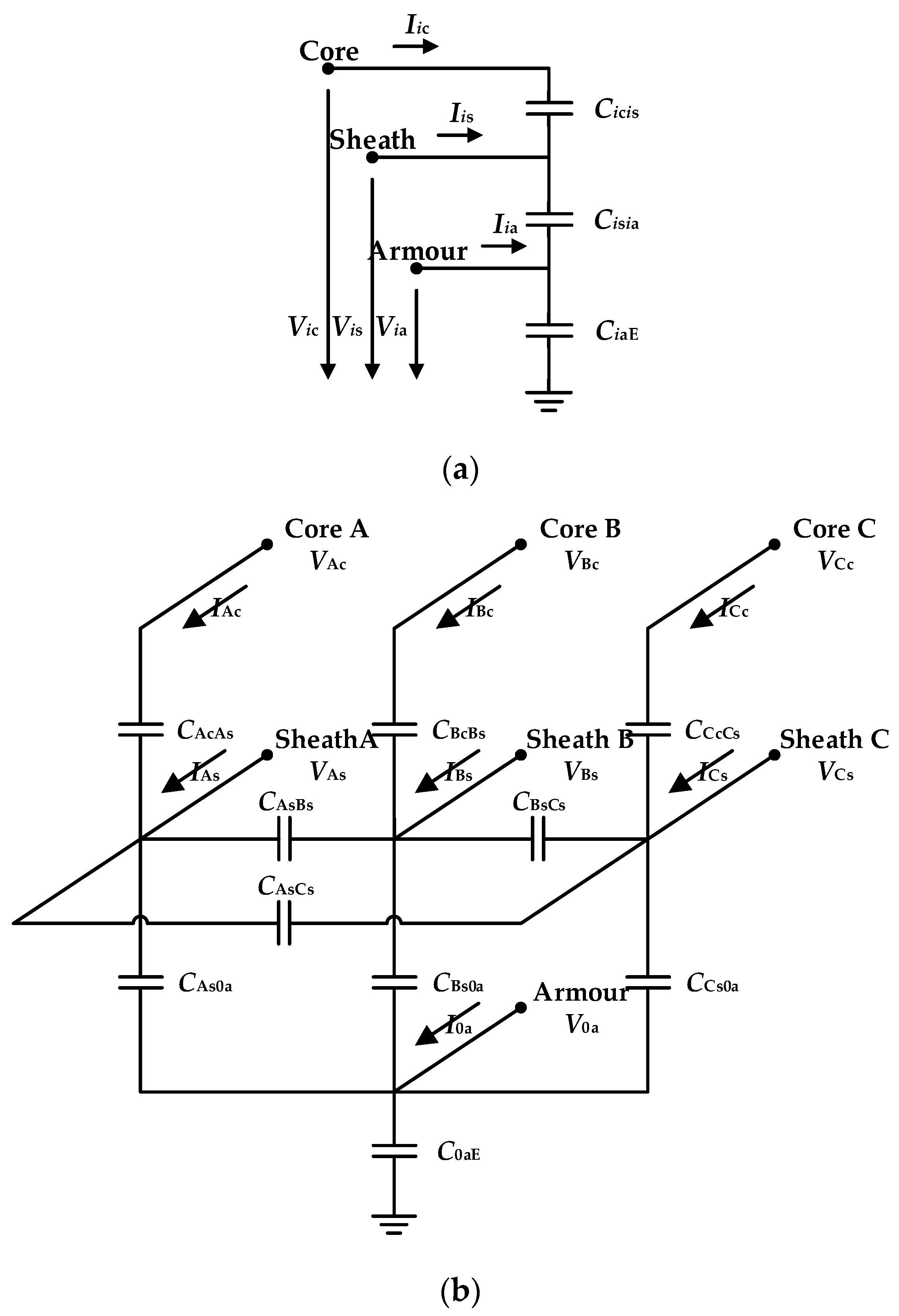
3.5. Construction of FSAM

Since the shunt conductances of the cables, caused by leakage currents, are very small and negligible, the shunt admittances can be considered to consist only of the shunt capacitances.

For single-core cables, the earth/sea connected to the sheaths and armors acts as electrostatic shielding, preventing capacitance between conductors of different phases. The shunt current equation is given as (38) [15], and its derivation can be found in Appendix B. In the equation, Y_Full is the FSAM; C_icis, C_isia, and C_iaE are the capacitances between the conductors.

$$\begin{array}{l}\left[\begin{array}{c}{I}_{\mathrm{Ac}}\\ I_{\mathrm{Bc}}\\ I_{\mathrm{Cc}}\\ I_{\mathrm{As}}\\ I_{\mathrm{Bs}}\\ I_{\mathrm{Cs}}\\ I_{\mathrm{Aa}}\\ I_{\mathrm{Ba}}\\ I_{\mathrm{Ca}}\end{array}\right]=\mathrm{j}\omega \left[\begin{array}{ccccccccc}{C}_{\mathrm{AcAs}}& 0& 0& -C_{\mathrm{AcAs}}& 0& 0& 0& 0& 0\\ 0& C_{\mathrm{BcBs}}& 0& 0& -C_{\mathrm{BcBs}}& 0& 0& 0& 0\\ 0& 0& C_{\mathrm{CcCs}}& 0& 0& -C_{\mathrm{CcCs}}& 0& 0& 0\\ -C_{\mathrm{AcAs}}& 0& 0& \begin{array}{l}(C_{\mathrm{AcAs}}\\ +C_{\mathrm{AsAa}})\end{array}& 0& 0& -C_{\mathrm{AsAa}}& 0& 0\\ 0& -C_{\mathrm{BcBs}}& 0& 0& \begin{array}{l}(C_{\mathrm{BcBs}}\\ +C_{\mathrm{BsBa}})\end{array}& 0& 0& -C_{\mathrm{BsBa}}& 0\\ 0& 0& -C_{\mathrm{CcCs}}& 0& 0& \begin{array}{l}(C_{\mathrm{CcCs}}\\ +C_{\mathrm{CsC}\mathrm{a}})\end{array}& 0& 0& -C_{\mathrm{CsC}\mathrm{a}}\\ 0& 0& 0& -C_{\mathrm{AsAa}}& 0& 0& \begin{array}{l}(C_{\mathrm{AsAa}}\\ +C_{\mathrm{AaE}})\end{array}& 0& 0\\ 0& 0& 0& 0& -C_{\mathrm{BsBa}}& 0& 0& \begin{array}{l}(C_{\mathrm{BsBa}}\\ +C_{\mathrm{BaE}})\end{array}& 0\\ 0& 0& 0& 0& 0& -C_{\mathrm{CsC}\mathrm{a}}& 0& 0& \begin{array}{l}(C_{\mathrm{CsC}\mathrm{a}}\\ +C_{\mathrm{CaE}})\end{array}\end{array}\right]\left[\begin{array}{c}{V}_{\mathrm{Ac}}\\ V_{\mathrm{Bc}}\\ V_{\mathrm{Cc}}\\ V_{\mathrm{As}}\\ V_{\mathrm{Bs}}\\ V_{\mathrm{Cs}}\\ V_{\mathrm{Aa}}\\ V_{\mathrm{Ba}}\\ V_{\mathrm{Ca}}\end{array}\right]\\ \Rightarrow \left[\begin{array}{c}{I}_{\mathrm{c}}\\ I_{\mathrm{s}}\\ I_{\mathrm{a}}\end{array}\right]=\left[\begin{array}{ccc}{Y}_{\mathrm{cc}}& Y_{\mathrm{cs}}& Y_{\mathrm{ca}}\\ Y_{\mathrm{cs}}^{\mathrm{T}}& Y_{\mathrm{ss}}& Y_{\mathrm{sa}}\\ Y_{\mathrm{ca}}^{\mathrm{T}}& Y_{\mathrm{sa}}^{\mathrm{T}}& Y_{\mathrm{aa}}\end{array}\right]\left[\begin{array}{c}{V}_{\mathrm{c}}\\ V_{\mathrm{s}}\\ V_{\mathrm{a}}\end{array}\right]\Rightarrow \left[\begin{array}{c}{I}_{\mathrm{c}}\\ I_{\mathrm{sa}}\end{array}\right]=\left[\begin{array}{cc}{Y}_{\mathrm{cc}}& Y_{\mathrm{csa}}\\ Y_{\mathrm{csa}}^{\mathrm{T}}& Y_{\mathrm{ssaa}}\end{array}\right]\left[\begin{array}{c}{V}_{\mathrm{c}}\\ V_{\mathrm{sa}}\end{array}\right]\Rightarrow \left[\begin{array}{c}{I}_{\mathrm{c}}\\ I_{\mathrm{sa}}\end{array}\right]=Y_{\mathrm{Full}}\left[\begin{array}{c}{V}_{\mathrm{c}}\\ V_{\mathrm{sa}}\end{array}\right]\end{array}$$

(38)

The capacitance between the core and sheath of a single-core cable is calculated as follows:

$$C_{i\mathrm{c}i\mathrm{s}}={\displaystyle \frac{{\epsilon }_{i\mathrm{cs}}}{18\ln \left(\frac{r_{\mathrm{i}\_i\mathrm{s}}}{r_{\mathrm{o}\_i\mathrm{c}}}\right)}} \mathsf{\mu }\mathrm{F}/\mathrm{km}$$

(39)

The capacitance between the sheath and armor of a single-core cable is calculated as follows:

$$C_{i\mathrm{s}i\mathrm{a}}={\displaystyle \frac{{\epsilon }_{i\mathrm{sa}}}{18\ln \left(\frac{r_{\mathrm{i}\_i\mathrm{a}}}{r_{\mathrm{o}\_i\mathrm{s}}}\right)}} \mathsf{\mu }\mathrm{F}/\mathrm{km}$$

(40)

The capacitance between the armor and earth/sea for a single-core cable is calculated as follows:

$$C_{i\mathrm{aE}}={\displaystyle \frac{{\epsilon }_{i\mathrm{aE}}}{18\ln \left(\frac{r_{\mathrm{o}\_i\mathrm{a}}+t_{i\mathrm{ps}}}{r_{\mathrm{o}\_i\mathrm{a}}}\right)}} \mathsf{\mu }\mathrm{F}/\mathrm{km}$$

(41)

From (39)–(41), it can be seen that since the capacitance calculations do not involve the positional parameters, the capacitance between corresponding conductors of each phase is equal for cables with identical structural parameters. Additionally, the cable layout does not affect the form of Y_Full.

For a three-core cable, since the sheath shields the core in the same phase, there is no electrostatic coupling between the core and conductors in different phases. The shunt current equation is presented as (42) [15], which can be derived by referring to Appendix B. In the equation, C_icis, C_isjs, C_is0a, and C_0aE are the capacitances between the conductors.

$$\begin{array}{l}\left[\begin{array}{c}{I}_{\mathrm{Ac}}\\ I_{\mathrm{Bc}}\\ I_{\mathrm{Cc}}\\ I_{\mathrm{As}}\\ I_{\mathrm{Bs}}\\ I_{\mathrm{Cs}}\\ I_{0\mathrm{a}}\end{array}\right]=\mathrm{j}\omega \left[\begin{array}{ccccccc}{C}_{\mathrm{AcAs}}& 0& 0& -C_{\mathrm{AcAs}}& 0& 0& 0\\ 0& C_{\mathrm{BcBs}}& 0& 0& -C_{\mathrm{BcBs}}& 0& 0\\ 0& 0& C_{\mathrm{CcCs}}& 0& 0& -C_{\mathrm{CcCs}}& 0\\ -C_{\mathrm{AcAs}}& 0& 0& \begin{array}{l}(C_{\mathrm{AcAs}}+C_{\mathrm{AsBs}}\\ +C_{\mathrm{AsCs}}+C_{\mathrm{As}0\mathrm{a}})\end{array}& -C_{\mathrm{AsBs}}& -C_{\mathrm{AsCs}}& -C_{\mathrm{As}0\mathrm{a}}\\ 0& -C_{\mathrm{BcBs}}& 0& -C_{\mathrm{AsBs}}& \begin{array}{l}(C_{\mathrm{BcBs}}+C_{\mathrm{AsBs}}\\ +C_{\mathrm{BsCs}}+C_{\mathrm{Bs}0\mathrm{a}})\end{array}& -C_{\mathrm{BsCs}}& -C_{\mathrm{Bs}0\mathrm{a}}\\ 0& 0& -C_{\mathrm{CcCs}}& -C_{\mathrm{AsCs}}& -C_{\mathrm{BsCs}}& \begin{array}{l}(C_{\mathrm{CcCs}}+C_{\mathrm{AsCs}}\\ +C_{\mathrm{BsCs}}+C_{\mathrm{Cs}0\mathrm{a}})\end{array}& -C_{\mathrm{Cs}0\mathrm{a}}\\ 0& 0& 0& -C_{\mathrm{As}0\mathrm{a}}& -C_{\mathrm{Bs}0\mathrm{a}}& -C_{\mathrm{Bs}0\mathrm{a}}& \begin{array}{l}(C_{\mathrm{As}0\mathrm{a}}+C_{\mathrm{Bs}0\mathrm{a}}\\ +C_{\mathrm{Cs}0\mathrm{a}}+C_{0\mathrm{aE}})\end{array}\end{array}\right]\left[\begin{array}{c}{V}_{\mathrm{Ac}}\\ V_{\mathrm{Bc}}\\ V_{\mathrm{Cc}}\\ V_{\mathrm{As}}\\ V_{\mathrm{Bs}}\\ V_{\mathrm{Cs}}\\ V_{0\mathrm{a}}\end{array}\right]\\ \Rightarrow \left[\begin{array}{c}{I}_{\mathrm{c}}\\ I_{\mathrm{s}}\\ I_{0\mathrm{a}}\end{array}\right]=\left[\begin{array}{ccc}{Y}_{\mathrm{cc}}& Y_{\mathrm{cs}}& Y_{\mathrm{ca}}\\ Y_{\mathrm{cs}}^{\mathrm{T}}& Y_{\mathrm{ss}}& Y_{\mathrm{sa}}\\ Y_{\mathrm{ca}}^{\mathrm{T}}& Y_{\mathrm{sa}}^{\mathrm{T}}& Y_{\mathrm{aa}}\end{array}\right]\left[\begin{array}{c}{V}_{\mathrm{c}}\\ V_{\mathrm{s}}\\ V_{0\mathrm{a}}\end{array}\right]\Rightarrow \left[\begin{array}{c}{I}_{\mathrm{c}}\\ I_{\mathrm{sa}}\end{array}\right]=\left[\begin{array}{cc}{Y}_{\mathrm{cc}}& Y_{\mathrm{csa}}\\ Y_{\mathrm{csa}}^{\mathrm{T}}& Y_{\mathrm{ssaa}}\end{array}\right]\left[\begin{array}{c}{V}_{\mathrm{c}}\\ V_{\mathrm{sa}}\end{array}\right]\Rightarrow \left[\begin{array}{c}{I}_{\mathrm{c}}\\ I_{\mathrm{sa}}\end{array}\right]=Y_{\mathrm{Full}}\left[\begin{array}{c}{V}_{\mathrm{c}}\\ V_{\mathrm{sa}}\end{array}\right]\end{array}$$

(42)

The capacitance C_icis between the core and sheath of a three-core cable is still calculated using (39).

The capacitance between the sheaths of each phase in a three-core cable is calculated as follows:

$$C_{i\mathrm{sjs}}={\displaystyle \frac{{\epsilon }_{0\mathrm{sa}}}{18\ln \left(\frac{r_{\mathrm{i}\_0\mathrm{a}}}{2r_{\mathrm{o}\_i\mathrm{s}}}\right)}} \mathsf{\mu }\mathrm{F}/\mathrm{km}$$

(43)

The capacitance between the sheath and armor of a three-core cable is calculated as follows:

$$C_{i\mathrm{s}0\mathrm{a}}={\displaystyle \frac{{\epsilon }_{0\mathrm{sa}}}{18\ln \left[\frac{r_{\mathrm{i}\_0\mathrm{a}}^2-{\left(2r_{\mathrm{o}\_i\mathrm{s}}/\sqrt{3}\right)}^2}{r_{\mathrm{i}\_0\mathrm{a}}\times r_{\mathrm{o}\_i\mathrm{c}}}\right]}} \mathsf{\mu }\mathrm{F}/\mathrm{km}$$

(44)

The capacitance C_0aE between the armor and earth/sea for a three-core cable is still calculated using (41).

It can be observed through calculations that the capacitance between corresponding conductors of each phase is still equal.

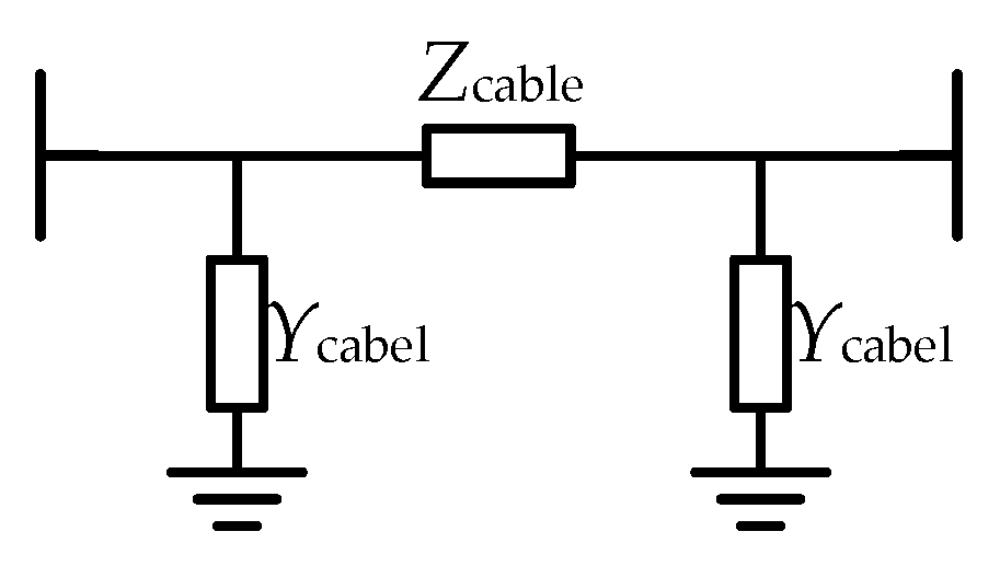
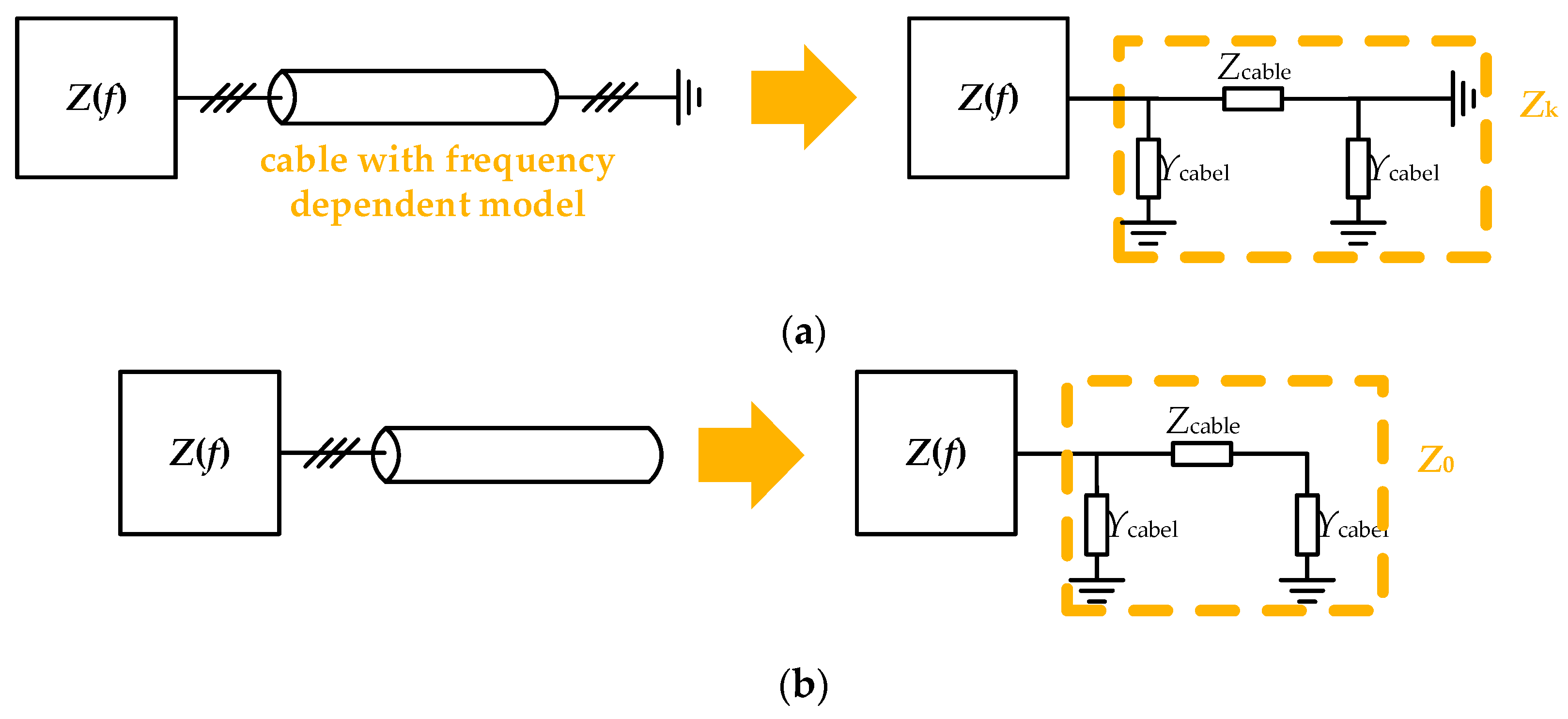
3.6. Transformation from FSAM to SSAM

Similarly, the analysis focuses on the core admittances, with the sheath and armor effects removed mathematically based on bonding and earthing methods.

For single-core cables with the solid bonding method, since V_sa = 0, (38) can be rewritten as follows:

$$\left[\begin{array}{c}{I}_{\mathrm{c}}\\ I_{\mathrm{sa}}\end{array}\right]=\left[\begin{array}{cc}{Y}_{\mathrm{cc}}& Y_{\mathrm{csa}}\\ Y_{\mathrm{csa}}^{\mathrm{T}}& Y_{\mathrm{ssaa}}\end{array}\right]\left[\begin{array}{c}{V}_{\mathrm{c}}\\ 0\end{array}\right]$$

(45)

Next, by eliminating I_sa, (45) can be rewritten as follows:

$$I_{\mathrm{c}}=Y_{\mathrm{cc}}{V}_{\mathrm{c}}=Y_{\mathrm{Phase}}{V}_{\mathrm{c}}$$

(46)

where Y_Phase is the PSAM.

For single-core cables with the single-point bonding method, since I_sa = 0, (38) can be rewritten as follows:

$$\left[\begin{array}{c}{I}_{\mathrm{c}}\\ 0\end{array}\right]=\left[\begin{array}{cc}{Y}_{\mathrm{cc}}& Y_{\mathrm{csa}}\\ Y_{\mathrm{csa}}^{\mathrm{T}}& Y_{\mathrm{ssaa}}\end{array}\right]\left[\begin{array}{c}{V}_{\mathrm{c}}\\ V_{\mathrm{sa}}\end{array}\right]$$

(47)

Next, by eliminating V_sa, (47) can be rewritten as follows:

$$I_{\mathrm{c}}=\left(Y_{\mathrm{cc}}-Y_{\mathrm{csa}}{Y}_{\mathrm{ssaa}}^{-1}{Y}_{\mathrm{csa}}^{\mathrm{T}}\right)V_{\mathrm{c}}=Y_{\mathrm{Phase}}{I}_{\mathrm{c}}$$

(48)

For single-core cables with the cross-bonding method, Y_cc is fully transformed as in (32)–(34), while Y_cs and Y_ca are partially transformed as in (35) and (36), respectively, forming a new Y_Full. Then, the new Y_Full is transformed into Y_Phase using (45) and (46).

The transformation from FSAM to PSAM for three-core cables is similar to (45) and (46).

The calculations show that Y_Phase is a diagonal matrix with equal diagonal elements, and the SSAM Y_ZPN equals Y_Phase after PST shown in (37).

4. Case Studies

4.1. Case Introduction

Calculate the electrical parameters for a three-core submarine cable and single-core submarine cables, with their parameters detailed in

Table 1. Parameters of three-core submarine cable.

Parameters of Conductors
Structure	Inner Radius/mm	Outer radius/mm	DC Resistivity/Ω·m
Core	0.00	18.90	1.7241 × 10−8
Sheath	47.30	51.00	2.14 × 10−7
Armor	120.65	126.65	1.38 × 10−7
Parameters of Insulations
Structure	Thickness/mm	Relative permittivity	Relative permeability
Core Insulation	28.40	2.25	1
Sheath Insulation	/	2.25	1
Armor Insulation	4.00	2.25	1
Positional Parameters
Average Burial Depth/m		10.00
Other Parameters
Cable Length/km		20.00
Sea DC Resistivity/Ω·m		0.50

and

Table 2. Parameters of single-core submarine cables.

Parameters of Conductors
Structure	Inner Radius/mm	Outer radius/mm	DC Resistivity/Ω·m
Core	0.00	17.10	1.7241 × 10−8
Sheath	46.40	50.30	2.14 × 10−7
Armor	62.20	68.20	1.38 × 10−7
Parameters of Insulations
Structure	Thickness/mm	Relative permittivity	Relative permeability
Core Insulation	29.30	2.25	1
Sheath Insulation	11.90	2.25	1
Armor Insulation	4.00	2.25	1
Positional Parameters
Average Burial Depth/m		10.00
Layout		Symmetrical Flat Layout
Adjacent Cable Axis Distance/m		200
Other Parameters
Cable Length/km		20.00
Sea DC Resistivity/Ω·m		0.50

, respectively. The target frequency range is 1~2000 Hz. It should be noted that the submarine cables are not twisted, and each single-core cable has the same average burial depth.

The case studies of three-core cables in different installation environments in Appendix C further verify the algorithm’s effectiveness.

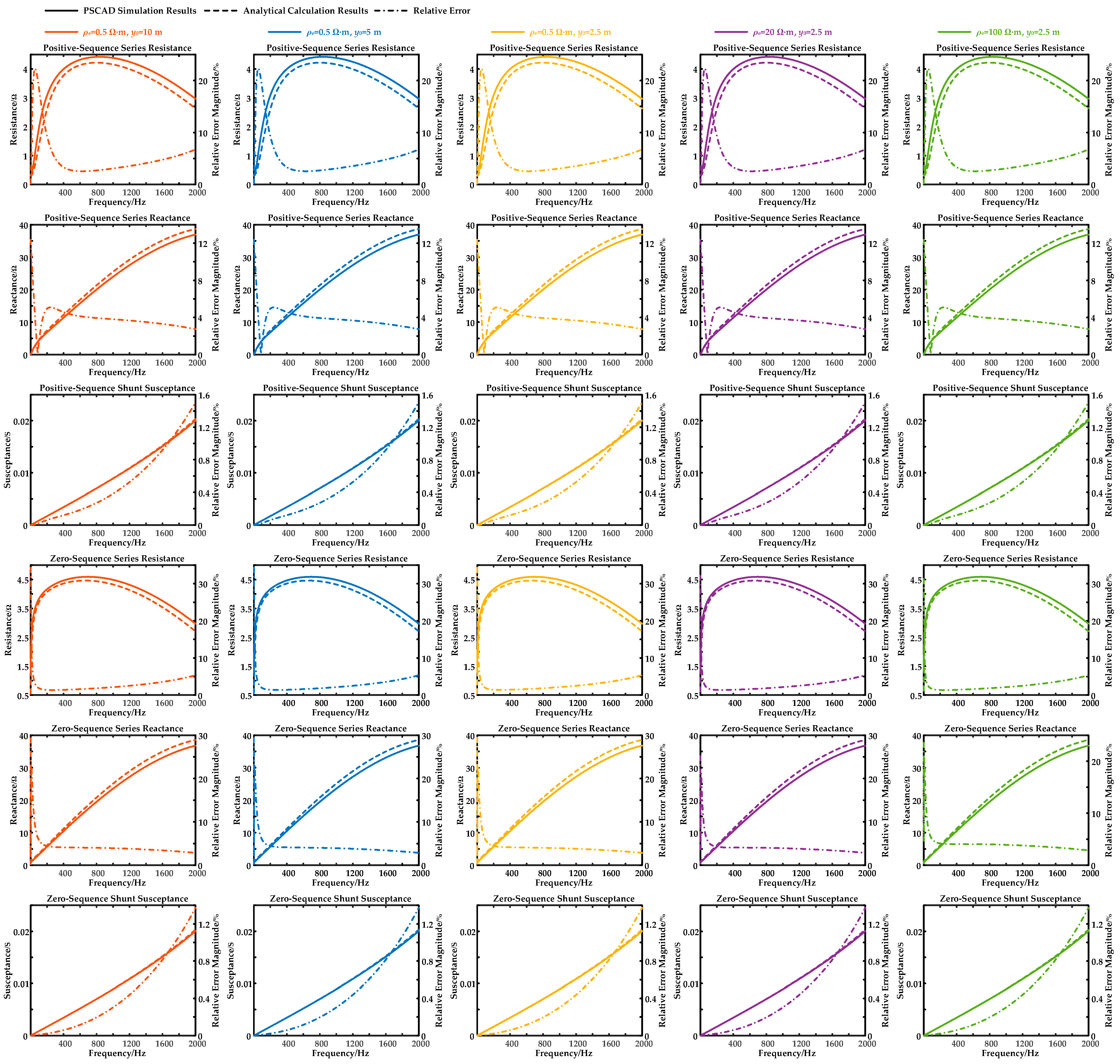
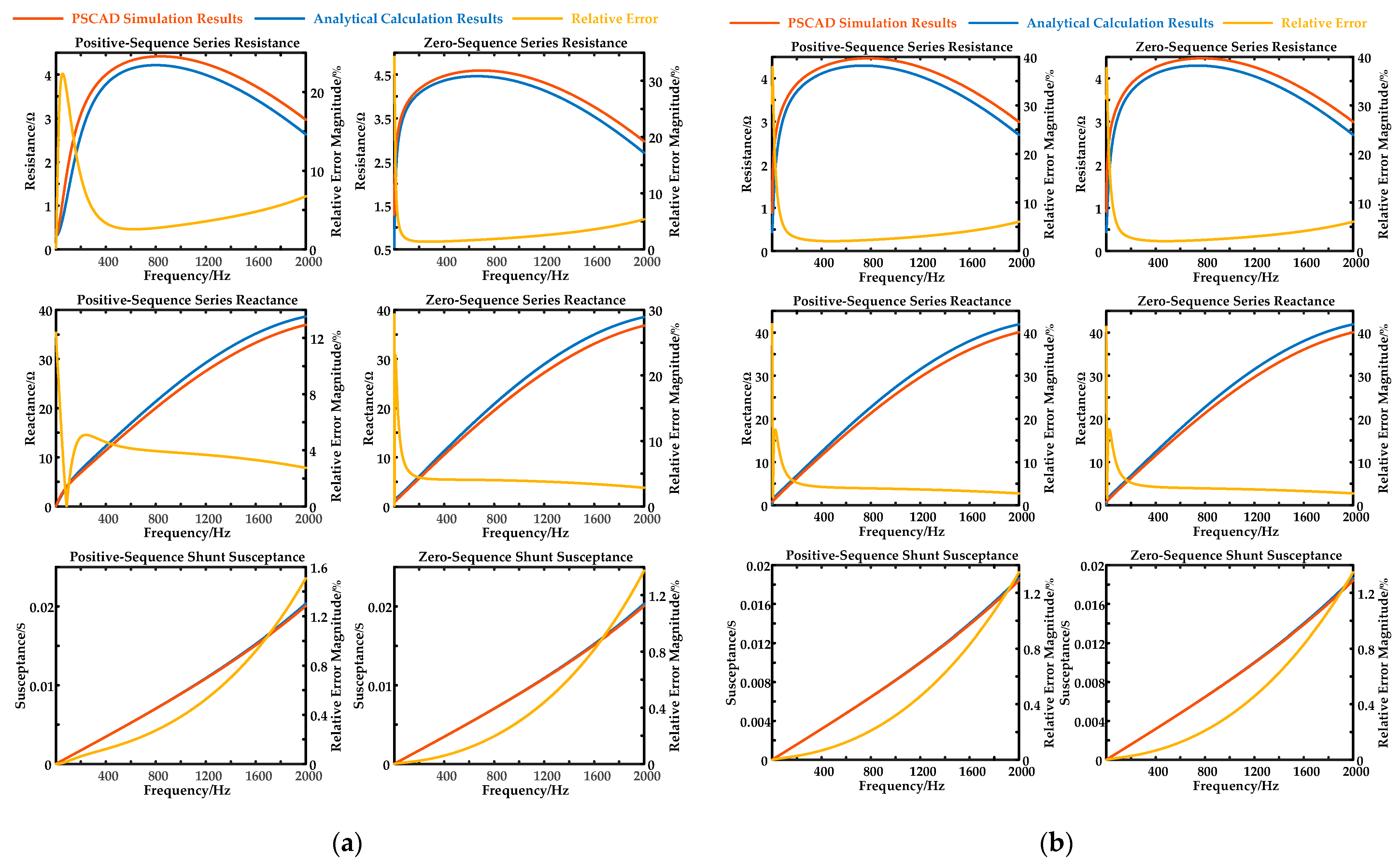
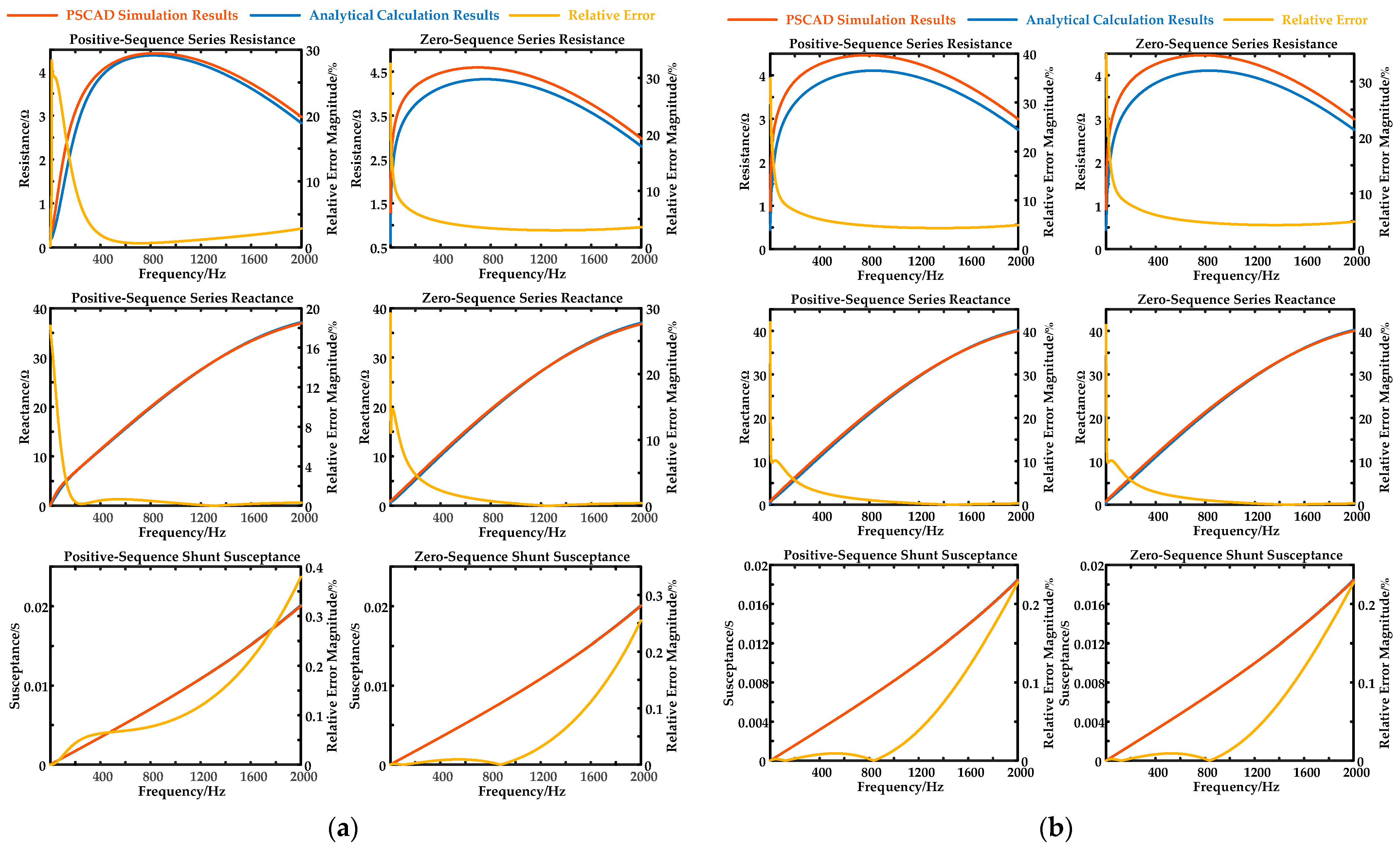
4.2. Simulation Verification

To verify the algorithm’s accuracy, apply the frequency-dependent model of cable in electromagnetic transient simulation software PSCAD/EMTDC 4.6.2 for comparison. The short-circuit impedance Z_k and open-circuit impedance Z₀ of the model are measured, as illustrated in Figure 9, and these two impedances satisfy the following relationships:

$$\left\{\begin{array}{l}{Z}_{\mathrm{k}}=\left(1/Y_{cable}\right)//Z_{cable}\hfill \\ Z_0=\left(1/Y_{cable}\right)//\left(Z_{cable}+1/Y_{cable}\right)\hfill \end{array}\right.$$

(49)

where // is the symbol used to calculate the parallel impedance. Thus, Z_cable and Y_cable are obtained by solving (49).

Since cables are static components, the positive-sequence and negative-sequence parameters are identical; the comparison focuses on Z_cable and Y_cable in the positive-sequence and zero-sequence π models. The comparison results for the three-core and single-core submarine cables are shown in Figure 10. The discussions are as follows:

1. For series resistances, the errors are larger at low frequencies, increase in the mid-to-high frequency range, but stay within an acceptable range.

2. For series reactances, the analytical results closely match the simulation ones. The relative errors are also higher at low frequencies and decrease at high frequencies, while the absolute errors increase with frequency.

3. For shunt susceptances, the errors are negligible across the entire frequency range.

4. Both series reactances and shunt susceptances increase with frequency, while series resistances increase at low-to-mid frequencies and decrease at high frequencies, primarily due to the characteristic of the parameter’s even distribution.

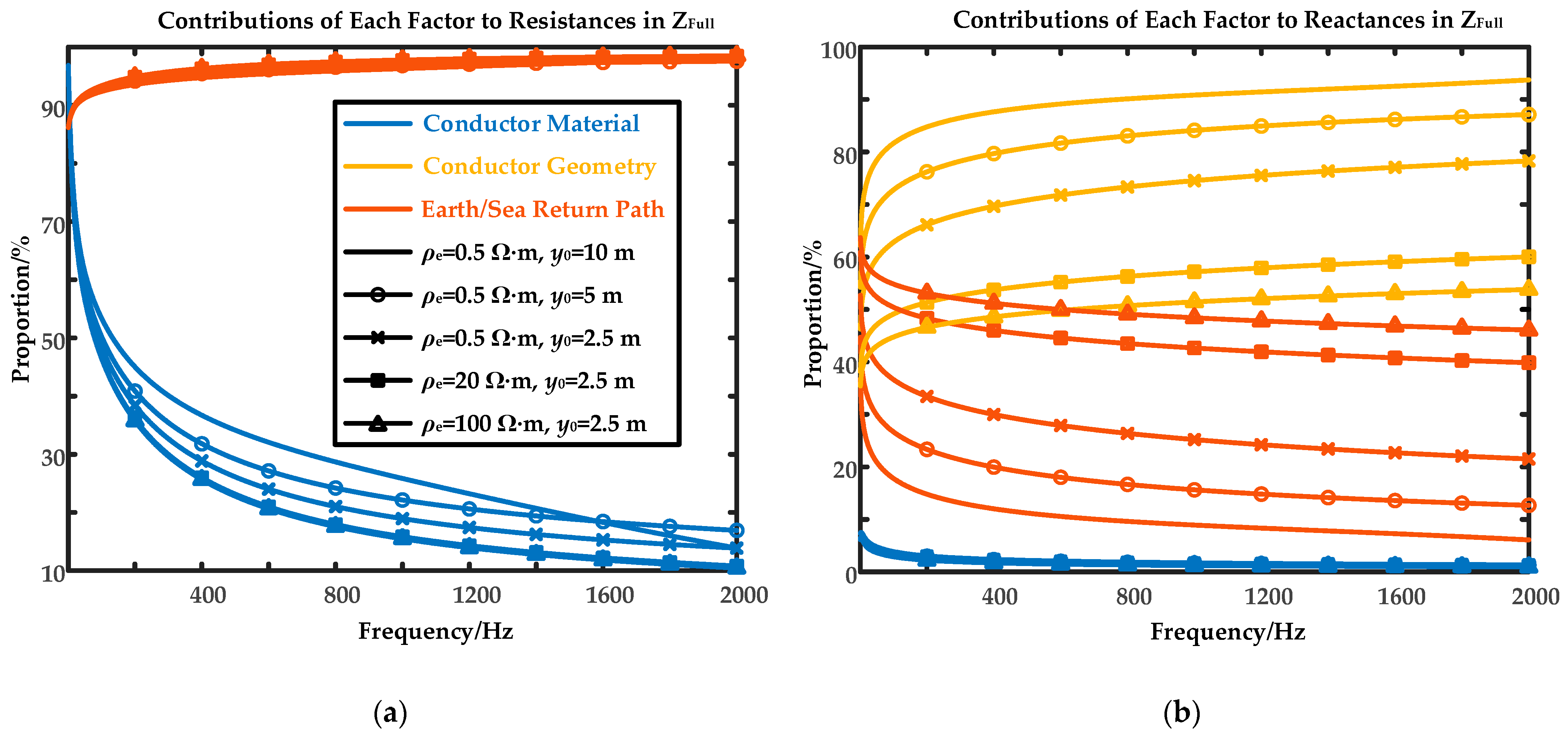
4.3. Analysis for Per-Unit-Length Parameters

Ignoring the cable length, the focus shifts to their per-unit-length parameters.

For per-unit-length shunt admittances, it is evident from the formulas of the shunt capacitances that they remain constant, independent of frequency. Therefore, the analysis concentrates on the per-unit-length series resistances and inductances.

The relationships of per-unit-length series resistances and inductances with frequency are illustrated in Figure 11. To explore the impacts of conductor material, conductor geometry, and earth/sea return path on per-unit-length series resistances and inductances, the contributions of each factor to the elements in Z_Full are defined as follows:

$$\left\{\begin{array}{l}{P}_{R\left(\mathrm{c}\right)}=\mathrm{mean}\left(R_{imim\left(\mathrm{c}\right)}/R_{imim\text{-}\mathrm{E}}\right)\hfill \\ P_{R\left(\mathrm{e}\right)}=\mathrm{mean}\left(R_{imjn\left(\mathrm{e}\right)}/R_{imjn\text{-}\mathrm{E}}\right)\hfill \end{array}\right.$$

(50)

$$\left\{\begin{array}{l}{P}_{X\left(\mathrm{c}\right)}=\mathrm{mean}\left(X_{imim\left(\mathrm{c}\right)}/X_{imim\text{-}\mathrm{E}}\right)\hfill \\ P_{X\left(\mathrm{g}\right)}=\mathrm{mean}\left(X_{imjn\left(\mathrm{g}\right)}/X_{imjn\text{-}\mathrm{E}}\right)\hfill \\ P_{X\left(\mathrm{e}\right)}=\mathrm{mean}\left(X_{imjn\left(\mathrm{e}\right)}/X_{imjn\text{-}\mathrm{E}}\right)\hfill \end{array}\right.$$

(51)

where P_R(c) and P_X(c) are the average contributions of the conductor material resistance R_imim(c) and reactance X_imim(c) to R_imim-E and X_imim-E, respectively; P_X(g) is the average contribution of the conductor geometry reactance X_imjn(g) to X_imjn-E; P_R(e) and P_X(e) are the average contributions of the earth/sea return path resistance R_imjn(e) and reactance X_imjn(e) to R_imjn-E and X_imjn-E, respectively; mean() is a function for calculating the average. Figure 12 shows the relationships between the above contributions of the three-core submarine cable and frequency, while similar results for the single-core submarine cables are not presented.

The per-unit-length series resistances increase rapidly with frequency at low-to-mid frequencies, mainly due to the comparatively larger contribution of the conductor material resistances, which rise with frequency as the skin effect. At high frequencies, the increasing rate of the per-unit-length series resistances slows down, with the resistances from the sea return path becoming absolutely dominant.

The per-unit-length series inductances decrease sharply with frequency at low-to-mid frequencies, caused by the reduction in the conductor material inductances due to the skin effect, as well as the decrease in the inductances from the sea return path. These two factors still contribute noticeably to this range. At high frequencies, the per-unit-length series inductances decrease extremely slowly, owing to the significant contribution of the conductor geometry inductances, which remain constant with frequency.

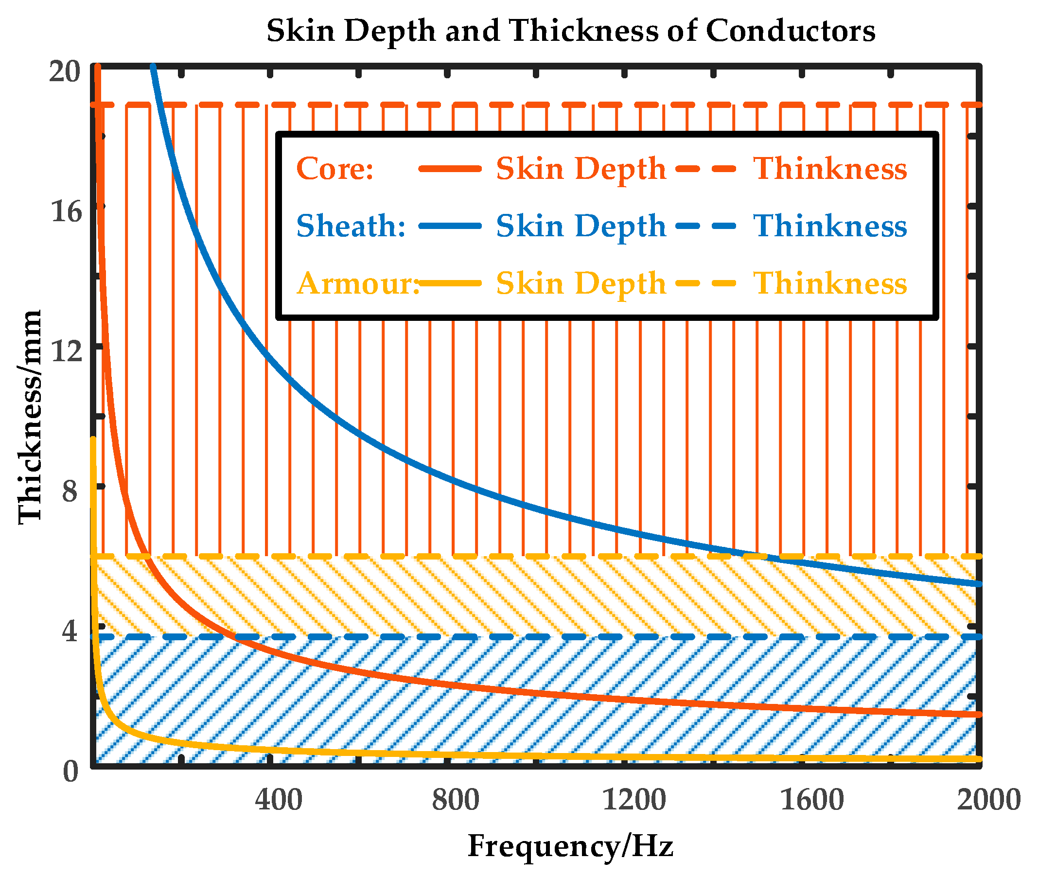
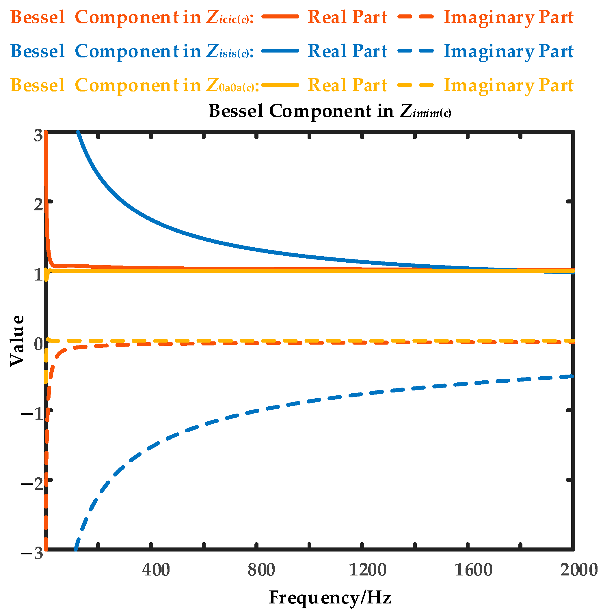
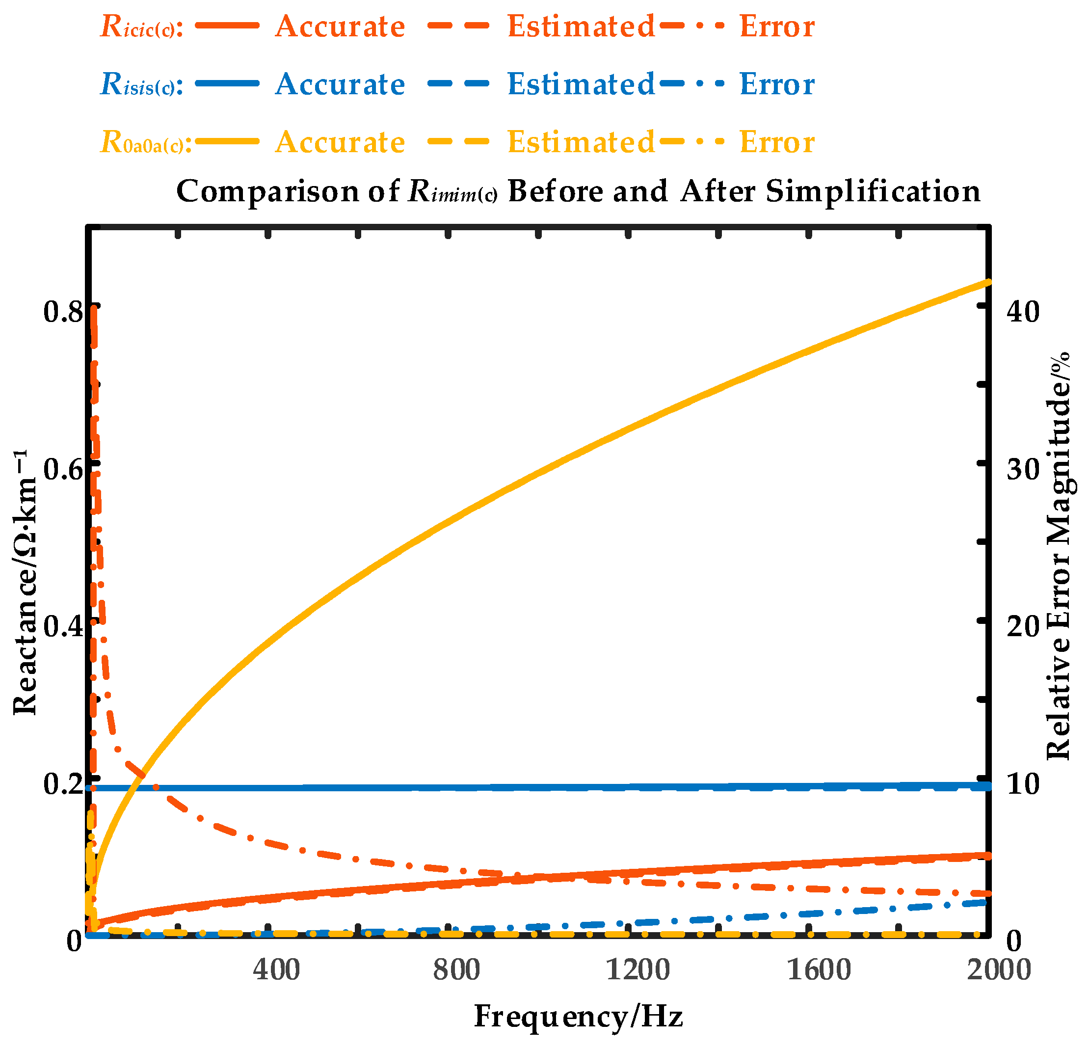
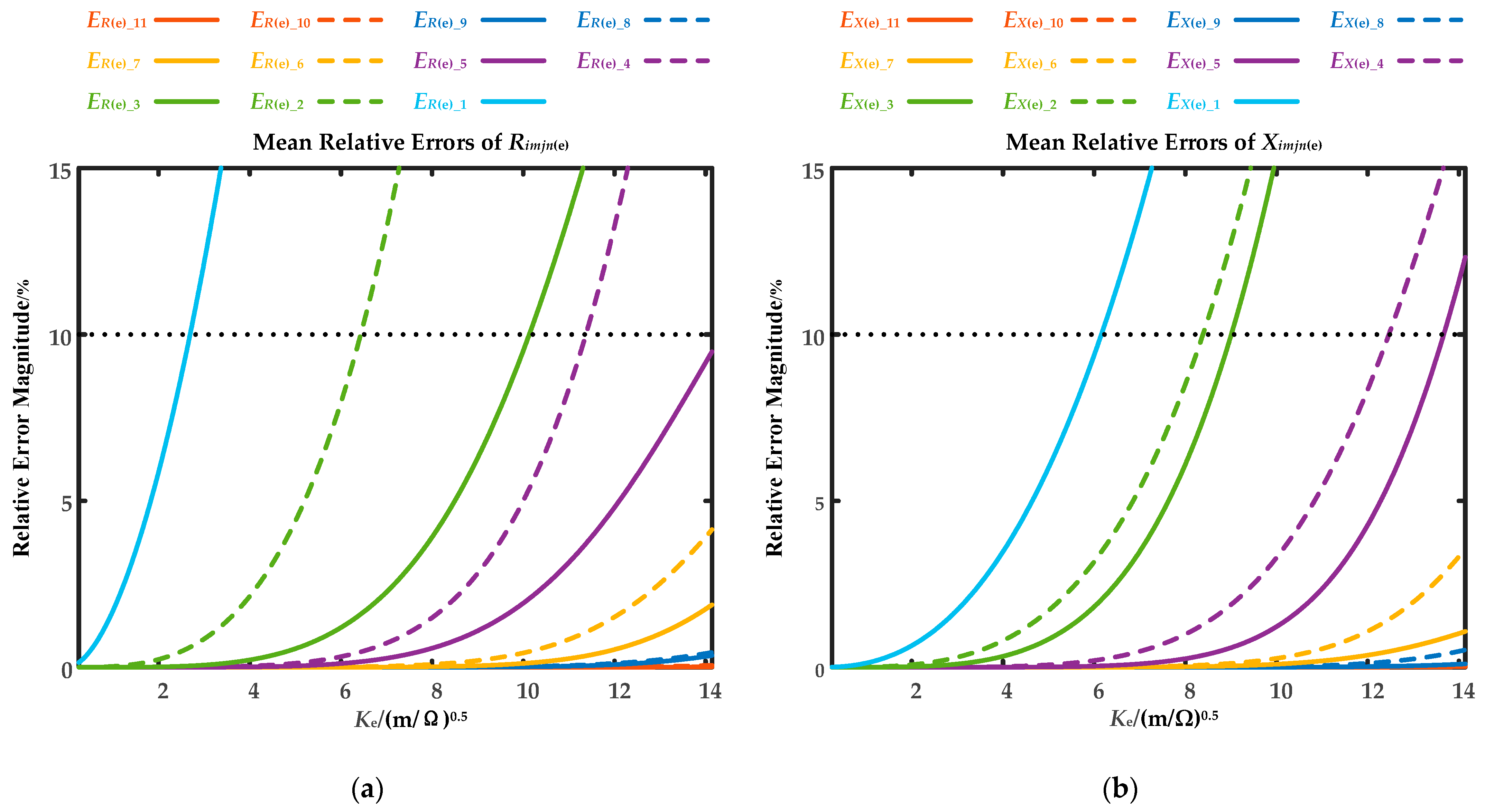
4.4. Exploration of Algorithm Simplification

The complex cable modeling necessitates simplified algorithms, with the exploration of simplification based on the three-core submarine cable case.

Further discussions on the relationships between the contributions of each factor to the impedances in Z_Full of the submarine cable and frequency are as follows:

1. For the contributions from the conductor material, P_R(c) decreases rapidly with frequency but still occupies a certain proportion in the low-to-mid frequency range, while P_X(c) is negligible across the entire frequency range.

2. For the contribution from the conductor geometry, P_X(g) increases with frequency and is a significant contribution to the reactances.

3. For the contributions from the sea return path, P_R(e) rises slightly with frequency and plays an important role in the resistances, while P_X(e) diminishes with frequency and has a relatively small influence on the reactances.

The variations in cable material and structural parameters generally have little impact on the contribution of each factor to the impedances in Z_Full, while changes in position and earth/sea return path parameters may have a significant effect. Thus, by varying the burial depth, i.e., the armor axis’ vertical coordinate y₀, and the DC resistivity of the return path resistivity ρ_e, the variations in each factor’s contribution to impedances are observed, with results plotted in Figure 12. The discussions of the results are as follows:

1. The changes in y₀ and ρ_e do not affect the trend of each factor’s contribution to impedances with frequency.

2. The magnitudes of P_R(c), P_X(c) and P_R(e) are insensitive to the changes in y₀ and ρ_e.

3. The magnitudes of P_X(g) and P_X(e) are notably influenced by the changes in y₀ and ρ_e. As y₀ decreases and ρ_e increases, P_X(e) rises, while P_X(g) represents the opposite trend.

The above analysis reveals that X_imim(c) can be neglected, while X_imjn(e) is also not significant in this submarine cable case but cannot be ignored for other positional and return path parameters. Additionally, R_imim(c) is relatively large at low-to-mid frequencies and cannot be removed. Therefore, calculating Z_imim(c) by considering only R_imim(c) is one of the keys for algorithm simplification.

According to the definition of skin depth, the AC resistance of the conductor can be estimated by the following equation:

$$R_{imim\left(\mathrm{c}\right)}=\left\{\begin{array}{l}{\displaystyle \frac{1000{\rho }_{\mathrm{c}\_im}}{\pi \left(r_{\mathrm{o}\_im}^2-r_{\mathrm{i}\_im}^2\right)}}\hspace{1em}{\delta }_{\mathrm{c}\_im}\ge \left(r_{\mathrm{o}\_im}-r_{\mathrm{i}\_im}\right)\hfill \\ {\displaystyle \frac{1000{\rho }_{\mathrm{c}\_im}}{\pi \left(2r_{\mathrm{o}\_im}{\delta }_{\mathrm{c}\_im}-{\delta }_{\mathrm{c}\_im}^2\right)}}\hspace{1em}{\delta }_{\mathrm{c}\_im}<\left(r_{\mathrm{o}\_im}-r_{\mathrm{i}\_im}\right)\hfill \end{array}\right.$$

(52)

where case 1 refers to when δ_{c_im} exceeds the conductor thickness, causing a uniform current distribution, with AC resistance equal to DC resistance; case 2 refers to when δ_{c_im} is smaller than the conductor thickness, with current concentrated in a ring with outer radius r_{o_im} and thickness δ_{c_im}.

By observing the relationship between the skin depth and thickness of each conductor in Figure 13, as well as the Bessel components in Z_imim(c) (I₀/I₁ in (17) and D₁/D₂ in (18)) in Figure 14, it can be found that as δ_{c_im} decreases, the Bessel component gradually converges. When δ_{c_im} is smaller than the conductor thickness, the Bessel component’s real part and imaginary part approach 1 and 0, respectively, allowing (17) and (18) to be simplified to (52), where δ_{c_im} is much smaller than r_{o_im}, and $r_{o\_im}^2$ can be neglected in comparison to 2δ_{c_im} r_{o_im}.

Furthermore, analyze the comparison of R_imim(c) before and after simplification in Figure 15. R_icic(c) and R_0a0a(c) increase with frequency across almost the entire range, as the skin depth of the core and armor is smaller than their thickness at low frequencies, with the Bessel components quickly converging, while R_isis(c) remains nearly constant as the sheath’s skin depth always exceeds its thickness. Importantly, the small errors in the AC resistance of the three conductors before and after simplification confirm the feasibility of estimation in (52).

Additionally, the expressions for R_imjn(e) and X_imjn(e) in (24) and (25) are infinite series, making the determination of the number of terms for R_imjn(e) and X_imjn(e) to retain under different y₀ and ρ_e another key in algorithm simplification. Clearly, the more terms retained, the higher the accuracy. In the above analysis, 12 terms are retained.

Z_imjn(e) is a function of λ_imjn and θ_imjn. For single-core cables, the dual variation of λ_imjn and θ_imjn makes the analysis difficult, so no simplification is applied. For a three-core cable, θ_imjn = 0, Z_imjn(e) depends only on λ_imjn. Thus, the following simplification of Z_imjn(e) applies only to three-core cables.

Substituting (22) into (23) and rearranging gives:

$${\delta }_{\mathrm{e}}={\displaystyle \frac{y_0}{\sqrt{{\rho }_{\mathrm{e}}}}}\cdot 2\sqrt{2\pi f{\mu }_{\mathrm{e}}}=K_{\mathrm{e}}\cdot 2\sqrt{2\pi f{\mu }_{\mathrm{e}}}$$

(53)

where K_e is the earth/sea return path position factor, in (m/Ω)^0.5.

As a result, Z_imjn(e) becomes a function of K_e. The studied range for y₀ and ρ_e is 2.5–10 m and 0.5–100 Ω·m, respectively, resulting in a range for K_e of 0.25–14.14 (m/Ω)^0.5.

To explore the impact of the number of retained terms on the accuracy, using Z_imjn(e) with 12 terms (Z_{imjn(e)_12}) as the reference, the mean relative errors of Z_imjn(e) with x (x < 12) terms (Z_{imjn(e)_x}) are calculated across the target frequency range, i.e.,

$$\left\{\begin{array}{l}{E}_{R\left(\mathrm{e}\right)\_x}=\left\{{\displaystyle \sum _{f=f_{\mathrm{st}}}^{f_{\mathrm{end}},\Delta f}\left[\left|R_{imjn\left(\mathrm{e}\right)\_x}\left(f\right)-R_{imjn\left(\mathrm{e}\right)\_12}\left(f\right)\right|/R_{imjn\left(\mathrm{e}\right)\_12}\left(f\right)\right]}\right\}/N_f\hfill \\ E_{X\left(\mathrm{e}\right)\_x}=\left\{{\displaystyle \sum _{f=f_{\mathrm{st}}}^{f_{\mathrm{end}},\Delta f}\left[\left|X_{imjn\left(\mathrm{e}\right)\_x}\left(f\right)-X_{imjn\left(\mathrm{e}\right)\_12}\left(f\right)\right|/X_{imjn\left(\mathrm{e}\right)\_12}\left(f\right)\right]}\right\}/N_f\hfill \end{array}\right.$$

(54)

where E_{R(e)_x} and E_{X(e)_x} are the mean relative errors of R_{imjn(e)_x} and X_{imjn(e)_x}, respectively; f_st and f_end are the start and end points of the target frequency range, respectively; Δf is the frequency step; N_f is the number of discrete frequencies.

The relationships between E_{R(e)_x}, E_{X(e)_x}, and K_e for different numbers of retained terms are shown in Figure 16. It is observed that, for the same number of retained terms, both E_{R(e)_x} and E_{X(e)_x} rise as K_e increases. An upper error limit of 10% is set to evaluate the accuracy, which can be adjusted based on the reader’s needs. The minimum number of retained terms for a given K_e that meets the error limit defines the terms to keep in the simplified algorithm. For y₀ and ρ_e in Table 1, five terms should be retained for R_imjn(e) and six terms for X_imjn(e) in the simplified algorithm.

Applying the simplified calculation, the π model parameters for the two submarine cables are shown in Figure 17. The acceptable errors demonstrate the accuracy of the impedance contribution analysis and the validity of the simplified algorithm that avoids the computations of Bessel functions and infinite series.

5. Conclusions

To accurately model cables in resonance stability analysis, this paper derives a concise analytical method for calculating cable electrical parameters over the wide frequency range. The main conclusions are as follows:

• The concise analytical method for cable modeling involves geometric parameter preprocessing, construction of full electrical parameter matrices, and transformation to sequence electrical parameter matrices based on bonding and earthing arrangements. The case studies of three-core and single-core submarine cables are presented to demonstrate the effectiveness of the improved analytical method.
• Cable series impedance arises from conductor material, conductor geometry, and earth/sea return path. The earth/sea return path significantly affects series resistance, while the conductor material’s influence decreases with frequency. Furthermore, conductor geometry and the return path contribute largely to series reactance, which is strongly dependent on the cables’ environment, while conductor material has little effect on series reactance.
• Cable per-unit-length series impedance’ frequency variation corresponds to that of its component contributions. At low-to-mid frequencies, series resistance increases rapidly while series inductance decreases sharply, both due to the conductors’ skin effect. At high frequencies, the rate of increase in series resistance and decrease in series inductance slows down, with the contribution from the earth/sea return path to series resistance and from the conductor geometry to series inductance becoming dominant.
• By ignoring the reactance from the conductor material and considering only its resistance, roughly estimated through the skin depth definition, this simplified algorithm proves feasible while avoiding the Bessel functions. Furthermore, for three-core cables, the earth/sea return path position factor helps determine the simplest series, avoiding the infinite series in the earth/sea return path impedance.

Although the cable modeling proposed in this paper is theoretically comprehensive and shows reasonably good accuracy in case validation, there are still some limitations:

• Single installation environment: The inhomogeneity of soil and seawater may lead to discrepancies between calculated and measured values. It is recommended to increase soil and seawater sampling points or use more accurate earth/sea return path impedance models. Additionally, variations in temperature and humidity can affect cable parameters (such as resistance and insulation performance), so it is advisable to make corrections for these factors in practical applications.
• Relatively “wide” frequency range: In power systems, resonance stability issues typically occur below 2 kHz, and harmonic analysis focuses on the 50–2500 Hz range. The proposed cable modeling provides good accuracy within these ranges, and the algorithm can be integrated into resonance stability analysis software for constructing the system’s node admittance matrix. However, for higher frequencies, such as those above 10 kHz, more precise modeling may be needed.

References

1. Benato, R.; Paolucci, A. EHV AC Undergrounding Electrical Power: Performance and Planning; Springer: New York, NY, USA, 2010; pp. 1–28. [Google Scholar]
2. Apostolaki-Iosifidou, E.; Mccormack, R.; Kempton, W.; Mccoy, P.; Ozkan, D. Transmission design and analysis for large-scale offshore wind energy development. IEEE Power Energy Technol. Syst. J. 2019, 6, 22–31. [Google Scholar] [CrossRef]
3. Taormina, B.; Bald, J.; Want, A.; Thouzeau, G.; Lejart, M.; Desroy, N.; Carlier, A. A review of potential impacts of submarine power cables on the marine environment: Knowledge gaps, recommendations and future directions. Renew. Sustain. Energy Rev. 2018, 96, 380–391. [Google Scholar] [CrossRef]
4. Bollen, M.; Yang, K. Harmonic aspects of wind power integration. J. Mod. Power Syst. Clean Energy 2013, 1, 14–21. [Google Scholar] [CrossRef]
5. Fillion, Y.; Deschanvres, S. Background harmonic amplifications within offshore wind farm connection projects. In Proceedings of the International Conference on Power Systems Transients (IPST 2015), Cavtat, Croatia, 15–18 June 2023; pp. 1–8. [Google Scholar]
6. Zhan, Y.; Xie, X.; Liu, H.; Liu, H.; Li, Y. Frequency-domain modal analysis of the oscillatory stability of power systems with high-penetration renewables. IEEE Trans. Sustain. Energy 2019, 10, 1534–1543. [Google Scholar] [CrossRef]
7. Xu, Z.; Wang, S.; Xing, F.; Xiao, H. Study on the method for analyzing electric network resonance stability. Energies 2018, 11, 646. [Google Scholar] [CrossRef]
8. Chen, Z.; Luo, A.; Kuang, H.; Zhou, L.; Chen, Y.; Huang, Y. Harmonic resonance characteristics of large-scale distributed powerplant in wideband frequency domain. Electr. Power Syst. Res. 2016, 10, 53–65. [Google Scholar]
9. Zhang, S.; Jiang, S.; Lu, X.; Ge, B.; Peng, F.Z. Resonance issues and damping techniques for grid-connected inverters with long transmission cable. IEEE Trans. Power Electron. 2014, 29, 110–120. [Google Scholar] [CrossRef]
10. Liu, Z.; Li, D.; Wang, W.; Wang, J.; Gong, D. A review of the research on the wide-band oscillation analysis and suppression of renewable energy grid-connected systems. Energies 2024, 17, 1809. [Google Scholar] [CrossRef]
11. Carson, J.R. Wave propagation in overhead wires with ground return. Bell Syst. Tech. J. 1926, 5, 539–554. [Google Scholar] [CrossRef]
12. Pollaczek, F. On the field produced by an infinity long wire carrying alternating current. Elektr. Nachrichtentechnik 1926, 3, 339–359. [Google Scholar]
13. Shelkunoff, S.A. The electromagnetic theory of coaxial transmission lines and cylindrical shields. Bell Syst. Tech. J. 1934, 13, 532–579. [Google Scholar] [CrossRef]
14. Wedepohl, L.M.; Wilcox, D.J. Transient analysis of underground power-transmission systems—System model and wave propagation characteristics. Proc. Inst. Electr. Eng. 1973, 120, 253–260. [Google Scholar] [CrossRef]
15. Ametani, A. A general formulation of impedance and admittance of cables. IEEE Trans. Power Appar. Syst. 1980, 99, 902–910. [Google Scholar] [CrossRef]
16. Tleis, N.D. Power Systems Modelling and Fault Analysis: Theory and Practice; Newnes: Oxford, UK, 2008; pp. 74–199. [Google Scholar]
17. Ruiz, C.; Abad, G.; Zubiaga, M.; Madariaga, D.; Arza, J. Frequency-dependent pi model of a three-core submarine cable for time and frequency domain analysis. Energies 2018, 11, 2778. [Google Scholar] [CrossRef]
18. Yin, Y.; Dommel, H.W. Calculation of frequency-dependent impedances of underground power cables with finite element method. IEEE Trans. Magn. 1989, 25, 3025–3027. [Google Scholar] [CrossRef]
19. Cristina, S.; Feliziani, M. A finite element technique for multiconductor cable parameters calculation. IEEE Trans. Magn. 1989, 25, 2986–2988. [Google Scholar] [CrossRef]
20. Darcherif, A.; Raizer, A.; Meunier, G.; Imfoff, J.; Sabonnadiere, J. New techniques in FEM field calculation applied to power cable characteristics computation. IEEE Trans. Magn. 1990, 26, 2388–2390. [Google Scholar] [CrossRef]
21. Habib, S.; Kordi, B. Calculation of multiconductor underground cables high-frequency per-unit-length parameters using electromagnetic modal analysis. IEEE Trans. Power Deliv. 2013, 28, 276–284. [Google Scholar] [CrossRef]
22. Arizon, P.D.; Dommel, H.W. Computation of cable impedances based on subdivision of conductors. IEEE Trans. Power Deliv. 1987, 2, 21–27. [Google Scholar] [CrossRef]
23. Feng, J.; Cheng, W. Calculation of cable electrical parameters considering proximity effect. In Proceedings of the 8th Asia Conference on Power and Electrical Engineering (ACPEE 2023), Tianjin, China, 14–16 April 2023; pp. 2174–2179. [Google Scholar]
24. Wakileh, G.J. Power Systems Harmonics/Fundamentals, Analysis and Filter Design; Springer: New York, USA, 2001; pp. 221–274. [Google Scholar]
Figure 1. Simplified structures of cables: (a) single-core cable; (b) three-core cable.
Electronics 14 01570 g001
Figure 2. Cables with the solid bonding method.
Electronics 14 01570 g002
Figure 3. Cables with the single-point bonding method: (a) the end-point bonding method; (b) the mid-point bonding method; (c) the end-point bonding method with an extra transposed conductor.
Electronics 14 01570 g003
Figure 4. Cables with the cross-bonding method.
Electronics 14 01570 g004
Figure 5. Typical layouts of Cables.
Electronics 14 01570 g005
Figure 6. π model of cable.
Electronics 14 01570 g006
Figure 7. Cable modeling process.
Electronics 14 01570 g007
Figure 8. Cables and their images: (a) Single-core cables; (b) three-core cable.
Electronics 14 01570 g008
Figure 9. Simulation verification: (a) Short-circuit test. (b) Open-circuit test.
Electronics 14 01570 g009
Figure 10. Comparison of parameters in the π model for cases with the complete algorithm: (a) three-core submarine cable; (b) single-core submarine cables.
Electronics 14 01570 g010
Figure 11. Relationships of per-unit-length parameters with frequency: (a) per-unit-length series resistances; (b) per-unit-length series inductances.
Electronics 14 01570 g011
Figure 12. Contributions of each factor to the impedances in ZFull of the three-core submarine cable: (a) resistance contributors; (b) reactance contributors.
Electronics 14 01570 g012
Figure 13. Skin depth and thickness of conductors in the three-core submarine cable.
Electronics 14 01570 g013
Figure 14. Bessel components of Zimim(c) in the three-core submarine cable.
Electronics 14 01570 g014
Figure 15. Comparison of Rimim(c) before and after simplification in the three-core submarine cable.
Electronics 14 01570 g015
Figure 16. Relationships between mean relative errors and Ke: (a) Rimjn(e); (b) Ximjn(e).
Electronics 14 01570 g016
Figure 17. Comparison of parameters in the π model for cases with the simplified algorithm: (a) three-core submarine cable; (b) single-core submarine cables.
Electronics 14 01570 g017