Abstract
Future power generation plants will be largely based on renewable energy sources such as wind or photovoltaic power. These plants are connected to the grid through power electronic converters, which may present stability problems, specifically in weak grids. Consequently, numerous stabilities studies have been conducted. In these studies, converters work as inverters; however, in power electronic interfaced loads, energy storage systems or High-Voltage Direct Current (HVDC) links, power converters can also function as a rectifier. Stability studies focusing on the rectifier operation have received little attention in previous research. In this paper, the Voltage Source Converter (VSC) stability is analysed for both the inverter and rectifier modes, with particular focus on the influence of the Phase-Locked Loop (PLL) and the current controllers’ bandwidths. Additionally, a Two-Degree-of-Freedom Proportional Integral (2DOF-PI) controller is proposed to expand the stable operating range. The stability study is carried out using a small-signal model validated through PSCAD simulations. The results show that for inverter operations, a slow PLL and fast current controllers yield better performance, whereas for rectifier operation, a fast PLL and slow current controllers are recommended. Finally, a robustness study based on the -norm is carried out to provide some tuning recommendations for the controller parameters, confirming the different behaviour in inverter and rectifier operation.
1. Introduction
The European Union (EU) aims to attain a minimum share of 42.5% of renewable energy in total energy consumption by 2030 [1]. Meeting this objective will heavily rely on electric power systems given their capacity to integrate renewable energy sources. For instance, the Spanish National Integrated Plan of Energy and Climate (PNIEC) has set an objective of 81% for the renewable energy generation in the Spanish power system by 2030 [2]. In this context, generation is shifting from conventional power plants based on synchronous generators to renewable power plants driven by power electronics.
Future power systems will, therefore, be dominated by inverter-based generation (IBG). However, this transition introduces some challenges, as identified by the Transmission System Operators (TSOs), including a reduction in the system inertia, lower transient stability margins, subsynchronous and harmonic resonances and synchronisation of the IBGs with the main grid [3,4]. These stability issues can be classified at the converter level, multiple converter level and system level [5]. Among the converter-level stability problems, weak grid-connected instability is emerging in grids with little or no synchronous generation, which reduces the short circuit ratio (SCR) [6,7].
Although grid-forming (GFM) converters are envisaged as a promising solution for future power grids to overcome some stability challenges [8], at present, Voltage Source Converters (VSCs) are still equipped with grid-following (GFL) controls, typically PI controllers in a synchronous reference frame (SRF) to regulate the active and reactive power [9]. However, GFL converters are more prone than GFM converters to present instability problems in weak grids [10]. Several studies have already analysed the main factors affecting the stability [11,12,13], highlighting that reduced active power, lower Phase-Locked Loop (PLL) bandwidths, reactive power injection or smaller electrical distances are beneficial for system stability. Simultaneously, various instability mitigation methods such as passive filters, active damping, increase in the grid strength, set-point adjustment or controller parameterisation have been proposed [14]. Among them, most of the research proposals are mainly focused on controller tuning since it is the easiest and most affordable solution.
The authors of [11] analysed the impact of system resistances on stability, finding that line resistances can provide positive damping, thereby improving the system stability, whereas converter resistances worsen it. The interactions among the PLL, inner current and outer power controllers are examined in [15], highlighting that, in weak grids, the controllers cannot be designed independently due to their interdependencies. Additionally, the study defines a stability region for tuning the controller parameters to ensure safe operation.
When injecting current, the voltage at the point of common coupling (PCC) is unintentionally manipulated, affecting both the PLL measurements and the power control loop, resulting in an unintended positive feedback loop that deteriorates the converter stability in weak grids [16], especially when the integral time constants of the current controllers are small (i.e., for fast inner current controllers) [17]. This feedback loop, driven by the dependence of the current reference on the PCC voltage when computed from the power references, makes the system sensitive to voltage deviations. Although its impact can be mitigated through control strategies such as V/Q control strategies in high-voltage grids, it negatively affects the converter stability. A virtual impedance for enhancing the stability of VSC in weak grids is proposed in [18]. The authors of [19] compared the stable operating zones of vector current control (VCC) and power synchronisation control (PSC), concluding that power synchronisation control is superior when the VSC is connected to weak grids.
The PLL, needed to obtain the voltage angle in GFL converters, is identified as one of the main destabilising factors, requiring lower PLL bandwidths as the SCR decreases [13,20,21]. In [16], several instability sources are analysed, and a design methodology using a PLL-free strategy for minimising the SCR level at which the VSC can operate is presented. Similarly, the PSC utilises an internal synchronisation mechanism similar to the operation of a synchronous machine to avoid PLL-induced instability in weak grids [22]. To enhance stability, a variable virtual impedance to increase the damping ratio of the PLL and an adaptive coefficient control is proposed in [23]. An adaptive PLL where the parameters of the PI controller are adjusted online according to the measured grid impedance is proposed in [24]. Reducing the PLL bandwidth as the grid strength decreases helps ensure stability but slows the transient response.
Power electronic-based loads are gaining importance in power systems, where the power converters operate as rectifiers rather than inverters. Other applications, such as battery energy storage systems or embedded modular multilevel converter (MMC)-based HVDC links, which require bidirectional power flow, will also become more prevalent in future power systems. In these cases, power converters can work in both modes, that is, rectifier and inverter modes [25,26].
At present, since most power converters are associated with renewable power plants, previous studies typically consider the inverter operation but not the rectifier operation. In this paper, the VSC stability when operating as a rectifier is analysed and compared to its operation as an inverter, highlighting the different impacts that the current and PLL controller bandwidths in both operating modes have on the stability. For the current controllers, the influence of the weighting factor used in Two-Degree-of-Freedom Proportional Integral (2DOF-PI) controllers is also analysed for both operating modes. These controllers enhance performance by decoupling control of the reference and plant dynamics, leading to better stability, faster responses, and enhanced robustness [27]. Additionally, a robustness study based on the -norm of the sensitivity transfer function matrix is proposed to determine those combinations of PLL and current controller bandwidths that ensure not only a stable operation but also an appropriate dynamic response. The results of this work show that the design rules for the current and PLL controllers are entirely dependent on the operating mode. While in the inverter operation, a slow PLL and fast current controllers provide a better dynamic response, in rectifier operation, a fast PLL and slow current controllers are required. Regarding the weighting factor of 2DOF-PIs, it is found to have a negligible impact on inverter operation. However, in inverter operation, it significantly affects stability, with a low value being beneficial.
The rest of the paper is organised as follows: Section 2 describes the system, which consists of a VSC connected to a weak grid, and Section 3 develops the small-signal state-space model used for the stability studies. A stability analysis of both rectifier and inverter operation is conducted in Section 4, highlighting the differences in terms of stability between both operating modes. A robustness study based on the -norm is carried out in Section 5. Finally, some concluding remarks including some tuning recommendations for the controller parameters are provided in Section 6.
2. System Description
Figure 1 shows the system under study, which consists of an 8 MW VSC converter, an output LC filter (, , , ), a 9.2 MVA step-up 0.690/66 kV transformer (, ) and a 66 kV ac grid modeled by its Thévenin impedance ( and ). Considering a two-level converter with a switching frequency of 2500 Hz, the filter is designed to reduce the current ripple below 2% of the rated current, with a resonant frequency at 769.5 Hz. Further details can be found in [28]. The system parameters are presented in Table 1.
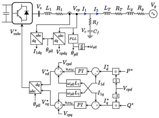
Figure 1.
Grid-following VSC model.

Table 1.
System parameters.
A standard grid-following control based on vector current control in the synchronous reference frame is used. The active and reactive power references are converted into d and q axis current references, respectively, and two 2DOF-PI controllers along with feed-forward terms determine the voltage to be generated by the converter.
The angle of the PCC voltage () is obtained by means of a PLL based on the synchronous reference frame, shown in Figure 2. It determines the grid angle by controlling the q-axis voltage to zero (). Thus, the PCC voltage is aligned with the d-axis of the SRF. The closed-loop transfer function of the PLL is
where and are the proportional and integral gains of the controller. These values can be calculated by comparing (1) with the transfer function of a second-order system, as carried out in [15,20]:
where is the damping factor and is the natural frequency.
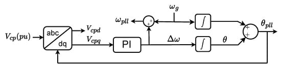
Figure 2.
Scheme of the SRF-PLL.
Figure 3 shows the current control loop, which employs 2DOF-PIs. The closed-loop transfer function is
where and are the proportional and integral gains of the current controllers and b is the reference weighting factor.
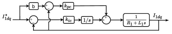
Figure 3.
Current control loop with 2DOF-PI.
To tune the current controllers, the methodology employed in this work is analogous to that used for the PLL, in which the closed-loop transfer function in (4) is compared with a standard second-order form. If the zeros in the numerator are neglected, the settling time at 98% can be expressed approximately as
where and are the damping factor and the natural frequency of (4), respectively. Hence, by specifying a desired settling time and , it is possible to determine the proportional and integral gains that achieve the target response as
3. Small-Signal Model
In this section, the small-signal model is presented, which is then validated against EMT-PSCAD simulations.
3.1. State-Space Representation
The eigenvalue method is used in this paper to study the stability of the system. The state-space representation of the system is carried out in the synchronous reference frame dq, with the following state variables:
where and are the d- and q-axis VSC output currents, respectively; and are the transformer currents; and are the capacitor voltages. , and are the integral terms of the current and PLL PIs, respectively. is the angular difference between the SRF determined by the PLL and a reference frame rotating at the grid frequency:
where is the angular frequency determined by the PLL and is the grid frequency (see Figure 2).
The equations of the transformer and the grid, as a function of the states, are
where , and is the angular speed of the dq frame. Note that the last terms of Equation (9) refer to the d- and q-axis PCC voltages, respectively:
The equations of the filter capacitor are
The equations of the series filter branch, expressed in terms of the states, are
where and are the d- and q-axis voltages generated by the VSC, respectively.
Neglecting delays, the output VSC voltage can be considered to be equal to its reference, that is, and , where and are determined by the current PI controllers and the feed-forward terms (see Figure 1). In practice, short delays arise from sampling, control computation, and the discrete update of the PWM signals. However, these delays typically lie in the microsecond range, much smaller than the dominant dynamic time constants considered here, and can therefore be neglected in the small-signal analysis. Therefore, the output voltages of the VSC can be expressed in terms of the state variables as
where and are the VSC current references in the d- and q-axis.
The PLL equations, with the d-axis aligned on the PCC voltage, can be expressed as a function of the states as
where is the angular frequency deviation with respect to the grid frequency .
Even though the grid frequency is constant, in (9) and (11) cannot be regarded as constant during transients since . Therefore, the system is not linear. In the literature, two dq reference frames are commonly used, one rotating at a constant speed determined by the grid frequency () and another one rotating at the frequency obtained from the PLL (), which is not constant during transients [11,17,20]. Equations (9) and (11) are expressed in the synchronous reference frame rotating at so the equations are linear. Equations (14)–(16) are written in the PLL frame rotating at a variable speed; however, is not involved, so the equations are also linear. Nonetheless, this methodology requires a frame transformation of the state variables between both frames.
In this paper, only one frame rotating at the speed determined by the PLL is used (), so Equations (9) and (11) must linearise at an operating point denoted by subscript 0. Therefore, in Equations (9) and (11) and the angular frequency at the operating point where the system is linearised, , is .
The PLL aligns the d-axis of the SRF with the PCC voltage, so . The grid voltages can be written as (see Figure 4)
where is the line-to-ground value of the grid voltage and is the angle difference between the PCC and the grid voltages. Linearising Equation (19),
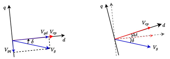
Figure 4.
Angle change of the grid voltage within the SRF-PLL.
The increase in the voltage angle difference (Figure 4) is the same as that measured by the PLL (). Moreover, assuming that the grid voltage amplitude does not change, Equation (20) can be simplified as
Taking into account that , and replacing (16) and (20) in (18), the expression for the transformer current is obtained:
Similarly, the non-linear terms and of Equation (11) are linearised as
Replacing (16) and (23) in (11),
In (14) and (15), the d- and q-axis current references are computed from the active and reactive power references, which can be expressed as a function of the states as
Linearising Equation (25),
Replacing (26) in (14), we obtain the linearised equation in terms of the power references:
Finally, replacing (26) in (15), the linearised equations are
The whole linearised system is described by Equations (16), (22), (24), (27) and (28). The state-space representation is
where the state (A) and input (B) matrices are
The input vector u is
3.2. Model Validation
To validate the state-space representation, the results of the small-signal model are compared with those obtained from PSCAD simulations (Figure 5). With the parameters presented in Table 2, the current controllers have a settling time of 20 ms and an overshoot lower than 4.3%. The bandwidth of the PLL is approximately 25 Hz.
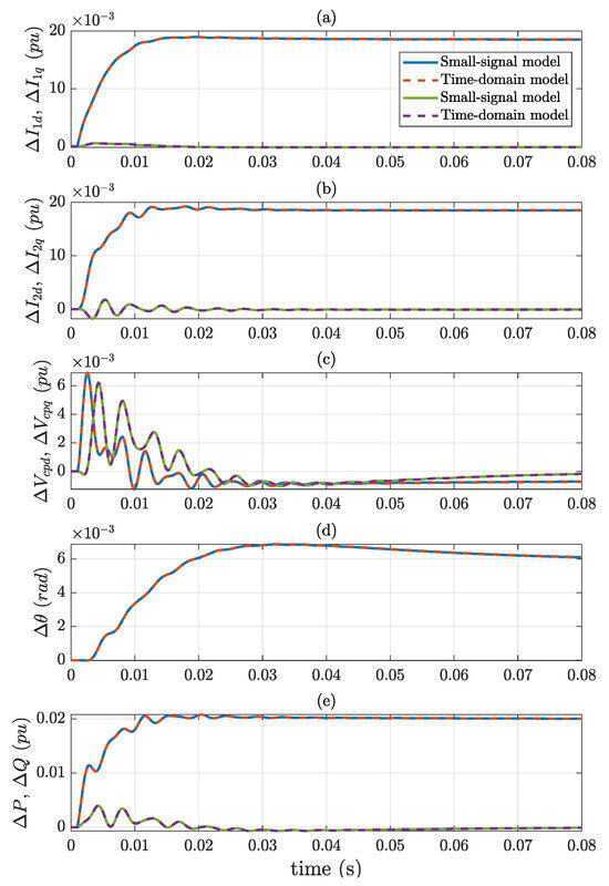
Figure 5.
Comparison of the small-signal and PSCAD results for a step change in P of 0.02 pu. From top to bottom: (a) d- and q-axis components of the converter current, (b) d- and q-axis components of the grid current, (c) d- and q-axis components of the PCC voltage, (d) PLL angle obtained from the integrator after the PLL-PI controller (see Figure 2), (e) active and reactive power at the PCC point.
Table 2.
System parameters for the small-signal model validation.
Initially, the converter generates MW (0.75 pu) and MVAr capacitive (0.25 pu), and at t = 2 ms, the active power is changed to 6.16 MW (0.02 pu step change). The values of the currents (, , , ), PCC voltage () and angle at the initial operating point are obtained by solving Equations (9), (10), (19) and (25), assuming that the derivative terms are zero (see Table 3).
Table 3.
Current, voltage and angle values at the operating point where the system is linearised.
Figure 5a,b show the d- and q-axis components of the output VSC and grid currents, respectively ( and in Figure 1). It can be seen that the d-axis current increases while the q-axis current remains unchanged since the d-axis of the synchronous reference frame is aligned with the PCC voltage. Figure 5c displays the d- and q-axis components of the PCC voltage. The q-axis component returns to zero due to the PLL control while the d-axis component is negative, meaning that the voltage at the PPC decreases due to a higher voltage drop caused by a higher current. The angle increase measured by the PLL is shown in Figure 5d. Finally, the active and reactive powers are depicted in Figure 5e. It can be noted that the results obtained from both models are superimposed during the whole transient, thereby validating the small-signal model.
4. System Stability
This section analyses the different impacts of the PLL and current controller design on the stability when the VSC operates as an inverter (injecting power) and rectifier (absorbing power).
4.1. PLL Bandwidth
Next, the effect of the PLL natural frequency, and by extension its bandwidth, on the stability is studied. The PLL damping ratio is fixed at , while the PLL natural frequency is changed. The parameters of the current controllers, unless otherwise stated, are those presented in Table 2.
4.1.1. Inverter Mode
Considering that the VSC generates pu and pu, Figure 6 shows the root locus plot for different PLL natural frequencies (10, 15, 20, 25 and 30 Hz) when the VSC is connected to a grid with an SCR of 2. It can be seen that as the PLL bandwidth increases, a pair of complex poles moves towards the positive plane, thereby destabilising the system. Hence, a high PLL bandwidth may destabilise the system when injecting power into the grid () as identified in other studies [11,20].
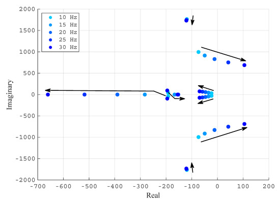
Figure 6.
Root locus for five PLL natural frequencies in inverter operation ( pu, pu and ).
A zoomed-in view of the root locus is shown in Figure 7, indicating system instability when the PLL natural frequency exceeds 21 Hz. For that value, the pair of complex poles is , that is, highly undamped poles () with an oscillating frequency of 129.5 Hz.
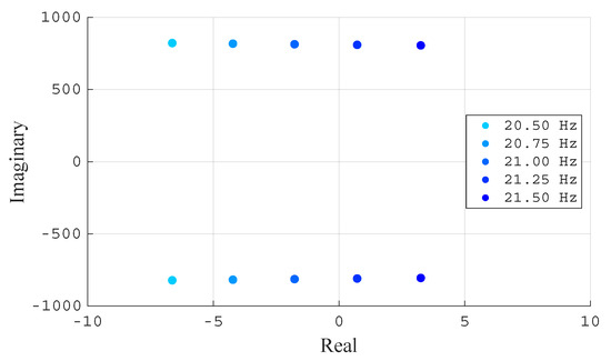
Figure 7.
Zoom-in of the root locus of Figure 6.
The same findings are obtained from the PSCAD model for two PLL designs with two different natural frequencies close to the stability limit, namely 20 and 21 Hz (Figure 8). The active power is changed from 0.99 to 1 pu at s, resulting in a very undamped but stable response for both PLL designs. When the power is increased to 1.01 pu at s, the system becomes unstable when the PLL natural frequency is 21 Hz with an oscillating frequency of 129.6 Hz. However, it is stable when the PLL natural frequency is 20 Hz. Therefore, both the small-signal model and PSCAD simulations consistently highlight the beneficial impact of a slower PLL on the system stability. Note that these simulations deliberately explore the limits of stability and are not intended to comply with interconnection standards (e.g., IEEE 1547 [29] or IEEE 2800 [30]). Therefore, neither of these controller designs would be acceptable in a real system. The goal here is to demonstrate the different behaviours of the rectifier and inverter that may make the system unstable rather than offer a fully compliant controller solution.
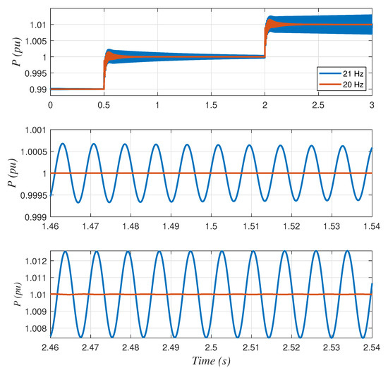
Figure 8.
PSCAD results for inverter mode (P > 0) with two PLL natural frequencies.
4.1.2. Rectifier Mode
The same analysis is repeated for the VSC rectifier operation. The VSC absorbs P = −1 pu and Q = 0 pu. Figure 9 shows the root locus plot for different PLL natural frequencies (10, 15, 20, 25 and 30 Hz) when the VSC is connected to a grid with an SCR of 3. Note that a pair of complex poles shifts from the positive plane to the negative plane when the PLL natural frequency increases, thereby stabilising the system. Hence, when the VSC operates as a rectifier (), a low PLL bandwidth may destabilise the system, in contrast to the behaviour observed in the inverter mode.
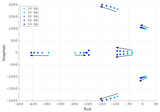
Figure 9.
Root locus for five PLL natural frequencies in rectifier operation (, and ).
Figure 10 shows a zoomed-in view of the root locus, revealing system instability when the PLL natural frequency is below 22.25 Hz. For that value, the pair of complex poles is , that is, highly undamped poles () with an oscillating frequency of 164.4 Hz.
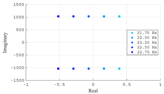
Figure 10.
Zoom-in of the root locus of Figure 9.
The same results are obtained from the PSCAD model for two PLL designs with two different natural frequencies close to the stability limit, namely 22.25 Hz and 25.25 Hz (Figure 11). The active power is changed from −0.99 to −1 pu at s, with both PLL designs being very undamped but stable. When the power is increased to −1.01 pu at s, the system becomes unstable when the PLL natural frequency is 22.25 Hz, with an oscillating frequency around 164 Hz. Conversely, it remains stable when the PLL natural frequency is 25.25 Hz. Therefore, both the small-signal model and PSCAD simulations consistently highlight the beneficial impact of a faster PLL on the system stability.
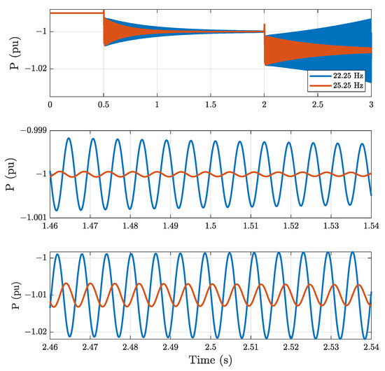
Figure 11.
PSCAD results for rectifier mode (P < 0) with two PLL natural frequencies.
Figure 8 and Figure 11 have been obtained from an ideal VSC model. The results using a detailed model considering PWM, dead times, delays and noise are presented in Appendix A. However, the conclusions regarding the impact of the PLL bandwidth remain the same.
4.2. Current Controllers
For the parameters of the current controllers presented in Table 4, Figure 12 shows the maximum PLL natural frequency as a function of the SCR for inverter mode. Similarly, Figure 13 shows the minimum PLL natural frequency as a function of the SCR for rectifier mode. Note that in Figure 12, the stable region is below the curves, whereas in Figure 13, the stable region is above the curves.
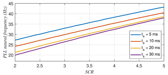
Figure 12.
Maximum PLL natural frequency as a function of the grid SCR and the current PI settling time in inverter operation (P = 1 pu, Q = 0 pu).
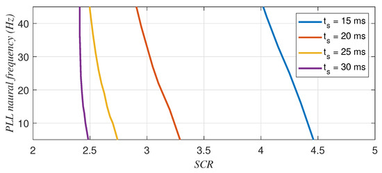
Figure 13.
Minimum PLL natural frequency as a function of the grid SCR and the current PI settling time in rectifier operation (P = −1 pu, Q = 0 pu).
In inverter mode (Figure 12), it can be seen that for higher SCRs, higher PLL bandwidths are allowed. For a given PLL design (natural frequency), faster current controllers can be connected to grids with lower SCRs. Moreover, the faster the current controller, the greater its impact (note that the difference between the 30 ms and 20 ms curves is smaller than the difference between the 20 ms and 10 ms curves).
In rectifier mode (Figure 13), it can be observed that higher SCRs allow for lower PLL bandwidths. For a given PLL design (natural frequency), slower current controllers enable connection to grids with lower SCRs. Moreover, the faster the current controller, the greater its negative impact (note that the difference between the 20 ms and 25 ms curves is larger than that between the 25 ms and 30 ms curves).
Again, the impact of the current controller differs in rectifier and inverter operation. While faster current controllers benefit the stability in inverter operation, they worsen the stability in rectifier mode.
4.3. Weighting Factor b of Current Controllers
This section analyses the influence of the reference weighting factor b of the 2DOF-PI on the system stability. This parameter attenuates the impact of the reference on the proportional action, reducing overshoot in transient responses. This adjustment is useful for improving the system’s response to reference changes without compromising disturbance rejection.
For inverter operation, Figure 14 shows the relation between the PLL natural frequency, the grid SCR and the parameter b for four settling times of the current controllers in Table 4. The weighting factor worsens the stability, with b = 1 being the best value regardless of the settling time of the current controller. The effect of the parameter b is more pronounced for faster current controllers. Thus, for inverter operation, the best choice is b = 1.
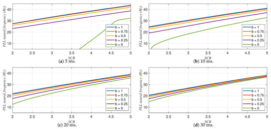
Figure 14.
Influence of the weighting factor b on the minimum SCR for 4 settling times of the current controllers. Inverter mode (P = 1 pu, Q = 0 pu).
Similarly, for rectifier operation, Figure 15 shows the relation between the PLL natural frequency, the grid SCR and the parameter b for four settling times of the current controllers. In contrast to the inverter operation, the weighting factor enhances the system stability, with lower values of b being the best choice regardless of the settling time of the current controller. The effect of the parameter b is more pronounced for faster current controllers.
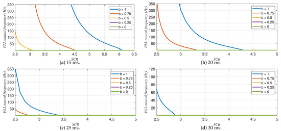
Figure 15.
Influence of the weighting factor b on the minimum SCR for 4 settling times of the current controllers. Rectifier mode (P = −1 pu, Q = 0 pu).
5. Robustness and Performance Analysis
The sensitivity function is widely recognised as a key indicator for assessing both the robustness and performance of a control system, as it represents the transfer function between the references and the corresponding errors. In a single-input single-output system, the -norm of is defined as the peak value of its frequency response. However, for multiple-input multiple-output systems, where is a transfer function matrix, the -norm is defined in terms of its singular values. Specifically, the -norm is given by
where denotes the maximum singular value. This definition captures the worst-case gain over all input directions. In this sense, higher values of the -norm indicate that the closed-loop system amplifies disturbances and uncertainties to a greater extent, which implies reduced robustness. Conversely, lower values suggest that the system is less sensitive to perturbations, thereby exhibiting enhanced robustness. A typical specification for robust performance is to constrain the sensitivity peak to a value around 2 [31], which helps to prevent excessive noise amplification at high frequencies while ensuring a quantifiable margin of robustness.
In the system under study, is defined as the function that has the active and reactive power references as inputs and the corresponding power-tracking errors as outputs. The power-tracking errors and for both active and reactive powers are computed as
As can be observed, Equation (34) shows non-linear expressions since some variables appear to be multiplied. Therefore, by linearising these equations, it is obtained that
Note that linearisation restricts the validity of the model to small deviations around the chosen operating point. This is standard practice in small-signal analyses, where the focus is on local stability rather than on large excursions or varying conditions. Here, the case of pu is examined (covering both inverter and rectifier operation) because higher power levels (in absolute value) generally translate into lower SCRs, representing a worst-case scenario for stability.
Then, the state-space model that defines the system under study and has the active and reactive power references u as inputs and the power-tracking errors y as outputs is
where matrices A and B are those defined in (30) and (31), and matrices C and D are
Hence, the sensitivity transfer function matrix is
and the peak of the maximum singular values of can be computed.
Regarding the performance analysis, it is conducted based on the system’s settling time at 98%. Given the system state-space representation defined by matrices A, B, C, and D, the settling time is estimated through the analysis of the eigenvalues of the state matrix A. Specifically, the dominant mode of the system is determined by the eigenvalue with the smallest absolute real part. Thus, the associated settling time at 98% can be approximated by
This estimation of the settling time is derived from the decay ratio associated with the dominant eigenvalue’s real part. It does not explicitly account for the damping factor, yet provides a practical measure of the dominant system behaviour and is considered sufficient for illustrative purposes.
To clearly illustrate how the parameters of the current controller and PLL affect both robustness and performance, several contour plots (from Figure 16, Figure 17, Figure 18 and Figure 19) are presented below. Robustness refers to the -norm defined in (33), while performance is assessed through defined in (40). The PLL parameters have been taken into account by using the natural frequency (in Hz), represented on the vertical axes, and the current controller parameters by using (in Hz), represented on the horizontal axes. is defined as , where is the damping factor (for all simulations in this work, a damping factor of has been employed) and is the natural frequency (as can be derived from (4), in Hz is ) of the closed-loop current control loop (see Section 2). All contour plots have been obtained by performing a parameter sweep of and with a sufficiently fine step size for both inverter and rectifier operating modes. Specifically, Figure 16 and Figure 17 show the impact of varying SCR values while keeping the weighting factor b fixed at 1, and Figure 18 and Figure 19 maintain a constant SCR value and vary the weighting factor b, clearly demonstrating how the adjustment of b significantly enhances robustness and performance. Presenting the results in this manner provides a visual and intuitive understanding of how the different parameters affect robustness and performance, offering practical insights into controller design considerations.
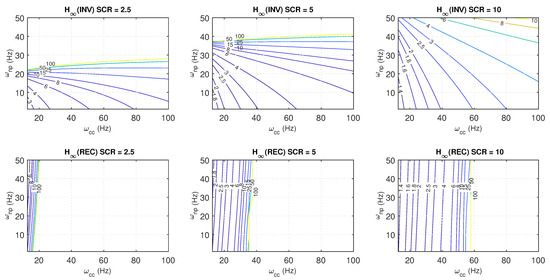
Figure 16.
-norm for inverter (top) and rectifier (bottom) operation for different values of SCR and the weighting factor .
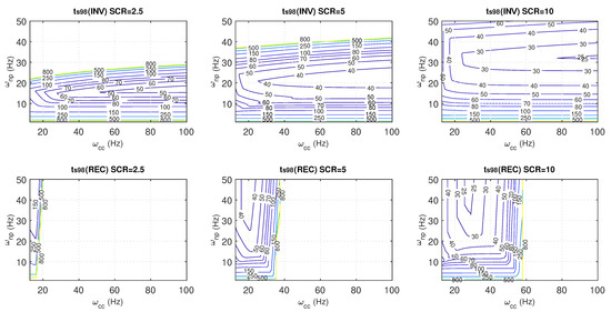
Figure 17.
Achieved settling times at 98% (in ms) for inverter (top) and rectifier (bottom) operation for different values of SCR and the weighting factor .
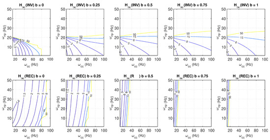
Figure 18.
-norm for inverter (top) and rectifier (bottom) operation for different values of the weighting factor b and SCR = 2.5.
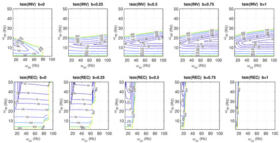
Figure 19.
Achieved settling times at 98% (in ms) for inverter (top) and rectifier (bottom) operation for different values of the weighting factor b and SCR = 2.5.
Figure 16 shows the contour plots of the norm values, which serve as the robustness metric, where for an acceptable performance, an -norm around 2 at most is considered [31]. The plots are generated for a sweep of PLL natural frequencies () and different closed-loop design frequencies of the current controller (), considering SCR values of 2.5, 5, and 10 for both inverter and rectifier modes. In both operation modes, the feasibility regions where the system remains stable reduce as the SCR decreases. In inverter mode, for a given current controller, faster PLLs tend to decrease robustness, eventually leading to instability beyond a certain limit. In contrast, in rectifier mode, faster PLLs slightly improve robustness (resulting in a lower ), while faster current controllers tend to reduce robustness and may induce instability. These results indicate that the PLL is the critical design element in inverter mode, with a slower PLL being favourable, whereas the current controller is more critical in rectifier mode, with slower controllers being interesting.
In weak grids, the achieved settling time may differ from that used to design the current controller due to variations in the PCC voltage during changes in active and reactive power, as well as potential oscillations in the current response if insufficient damping is provided. Figure 17 presents the achieved settling time at 98% (as defined in (40)) for the same conditions as in Figure 16, with the settling time derived from the dominant pole of the closed-loop system. It is observed that, for both operating modes, as the SCR decreases, the settling time increases and deviates further from the closed-loop time employed in the current controller design. In inverter mode, for a given current controller, an optimal PLL frequency exists that minimises the settling time, i.e., faster PLLs (or slower) lead to a slower system response. For instance, for SCR = 2.5, it can be observed that the PLL has a significant impact on the settling time. For a given , the fastest response is achieved with a PLL with a natural frequency around 15 Hz. If the PLL is faster or slower, the settling time of the current controller increases considerably. It is also observed that for a given PLL, faster controllers lead to smaller settling times; however, the speed of the response is much more influenced by the PLL design than the current controller parameters. Similarly, in rectifier mode, for a given PLL frequency, an optimal current controller minimises the achieved settling time and for a given controller, faster PLLs lead to smaller settling times and also improved robustness, with faster PLLs being favourable. However, in this case, the impact of the current controller is much more pronounced than that of the PLL.
For an SCR of 2.5 and a sweep of different values of the weighting parameter b (0, 0.25, 0.5, 0.75, and 1), the contour plots for the -norm (Figure 18) and the settling times (Figure 19) are presented for both inverter and rectifier modes. In inverter mode, reducing b generally results in lower -norm values. However, the size of the feasible (stable) regions also decreases as b is reduced. As noted previously, in inverter mode, the PLL is the most critical component, so for a given current controller, the minimum PLL frequency that triggers instability decreases slightly with a reduction in b. In this sense, adjusting b mainly affects performance (e.g., the oscillatory behaviour) rather than stability. For rectifier mode, the parameter b yields considerably greater improvements in stability. As b decreases, the feasible region expands and improved robustness is observed through lower -norm values. Regarding the achieved settling times, in addition to the conclusions drawn from Figure 17, it is observed that as b decreases, the settling times increase, indicating a slower overall system response that diverges further from the design values.
Figure 20 illustrates the time-domain responses in inverter and rectifier modes when the reference power changes from 0.95 pu to 1 pu (inverter) and from −0.95 pu to −1 pu (rectifier), considering an SCR of 2.5. The responses of four different controllers, as detailed in Table 5, are compared. Note that the same is used for all the controllers (25.5 Hz), which corresponds to a settling time of approximately 25 ms for the design of the current control loop. Therefore, in inverter mode, controllers with a slow PLL (C1 and C3) remain stable, with the weighting parameter b affecting only performance, as indicated by differences in oscillatory behaviour and settling times. In contrast, controllers with a fast PLL (C2 and C4) fall outside the feasible region, resulting in unstable system behaviour that cannot be corrected by adjusting b. For rectifier mode, controllers with a lower b value (C1 and C2) lead to a stable system response, with the PLL primarily influencing performance (with faster PLLs being more favourable). Controllers with (C3 and C4) fall outside the feasible region, leading to instability.
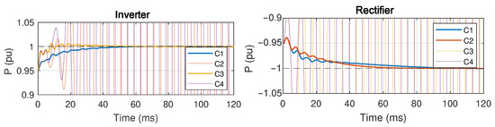
Figure 20.
Step response of four controllers (C1 to C4) to a power reference change in inverter and rectifier modes considering SCR = 2.5.
Table 5.
Comparison of controllers.
6. Conclusions
Numerous papers have studied the stability of VSCs connected to weak grids when operating as inverters. However, their stability when working as rectifiers has received little attention. This paper analyses the different impacts of the PLL and current controller parameters depending on the converter’s operation mode. The main findings are summarised as follows:
- During inverter operation, a low PLL bandwidth improves the system stability, enabling the connection of VSCs to weaker grids. Conversely, during rectifier operation, a high PLL bandwidth enhances the system stability.
- The settling time of the inner current control loops has a minor impact on the stability during inverter operation, with faster current controls only marginally increasing the stability. Conversely, faster current control loops significantly reduce the stability margins during rectifier operation, potentially leading to system instability.
- The reference weighting factor b of the 2DOF-PI used in the current loops has a minor impact on the stability during inverter operation, with smaller values of b worsening the stability. On the contrary, lower values of b improve the system stability during rectifier operation, with b having a significant impact.
- During rectifier operation, although a lower value of the parameter b reduces the stability limits, it enhances system performance for typical PLL and current controller design parameters by increasing the damping, consequently reducing oscillations.
The impacts of the PLL bandwidth, the settling time of the current control loops, and the reference weighting factor b have opposing effects on VSC stability when operating as a rectifier or inverter, results that have been validated through the root locus of the eigenvalues, the -norm of the sensitivity function and EMT-PSCAD simulations. Therefore, with the increasing number of VSCs working as rectifiers (e.g., HVDC links, energy storage systems, converter-interfaced loads), the typical design recommendations used for the inverter operation may not be valid for rectifier operation.
Author Contributions
Conceptualisation, R.V.-A., C.D.-S. and I.P.-A.; methodology, R.V.-A. and C.D.-S.; software, J.J.T.B.; validation, R.V.-A., J.J.T.B. and C.D.-S.; formal analysis, R.V.-A., C.D.-S. and I.P.-A.; investigation, R.V.-A., J.J.T.B., C.D.-S. and I.P.-A.; writing, R.V.-A., J.J.T.B. and C.D.-S.; supervision, R.V.-A. and I.P.-A. All authors have read and agreed to the published version of the manuscript.
Funding
The authors would like to acknowledge the support of the Spanish Research Agency through grant PID2020-112943RBI00 funded by MCIN/AEI/10.13039/501100011033; grant PID2021-125634OB-I00 funded by MCIN/AEI/10.13039/501100011033 and ERDF a way of making Europe; and grants TED2021-130120BB-C21 and TED2021-130120B-C22 funded by MCIN/AEI/10.13039/501100011033 and by the European Union NextGenerationEU/PRTR.
Data Availability Statement
The data are included in the article. Additional data are available from the corresponding author upon request.
Conflicts of Interest
The authors declare no conflicts of interest.
Abbreviations
The following abbreviations are used in this manuscript:
| 2DOF-PI | Two-Degree-of-Freedom Proportional Integral |
| GFL | Grid Following |
| GFM | Grid Forming |
| PI | Proportional Integral |
| PCC | Point of common coupling |
| PLL | Phase-Locked Loop |
| SCR | Short circuit ratio |
| VCC | Vector current control |
| VSC | Voltage Source Converter |
Appendix A
The results presented in Section 4 are obtained using an averaged ideal model of the VSC. To study the impact of delays, measurement filters, dead times and grid harmonics, a detailed model of a two-level converter has been developed. The switching frequency is 2500 Hz and the dead time is 7 s. The harmonic content of the grid voltage is 3rd harmonic (1%), 5th harmonic (2%), 7th harmonic (2%) and 15th harmonic (0.1%) according to real measurements in medium-voltage grids conducted by E.ON Distribution in the Czech Republic [32].
Figure A1 shows the results for a change in active power when the VSC works as an inverter. The SCR is 2 as in Section 4.1.1. Initially, the active and reactive powers are zero. From t = 0.1 s to t = 0.2 s, the power ramps up from 0 to 0.95 pu, and at t = 0.6 s, the power increases to 1 pu. Figure A1a and Figure A1b present the results for two designs of the PLLs with natural frequencies of 18 Hz and 23 Hz, respectively. The proportional and integral gains of the current controllers are those presented in Table 2. From top to bottom, both figures display the following variables: active power, grid-side current and grid voltage. As it is observed, a higher PLL natural frequency worsens the stability of the system. The system with a PLL with a lower natural frequency (Figure A1a) remains stable, whereas the other (Figure A1b) becomes unstable.
The same simulation has been repeated for the rectifier operation (Figure A2). The SCR is 3 as in Section 4.1.2. The changes in the active power are the same; however, the active power is now negative. The natural frequency of the PLL is 20 Hz (Figure A2a) and 30 Hz (Figure A2b). As observed, a higher PLL natural frequency enhances the stability of the system. Therefore, although the exact value of the SCR at which the VSC becomes unstable varies slightly with respect to the small-signal model, the conclusions drawn from the ideal model remain valid. A faster PLL worsens stability during the inverter operation while it improves the stability during the rectifier operation.

Figure A1.
Influence of the PLL natural frequency on the VSC stability when operating as an inverter. Left figure: Hz; right figure: Hz. From top to bottom: active power, grid-side current and grid voltage.

Figure A2.
Influence of the PLL natural frequency on the VSC stability when operating as a rectifier. Left figure (a) ; right figure (b) . From top to bottom: active power, grid-side current and grid voltage.
References
- Official Journal of the European Union. DIRECTIVE (EU) 2023/2413 Amending Directive (EU) 2018/2001, Regulation (EU) 2018/1999 and Directive 98/70/EC as Regards the Promotion of Energy from Renewable Sources. Available online: https://eur-lex.europa.eu/legal-content/EN/TXT/PDF/?uri=OJ:L_202302413 (accessed on 18 February 2025).
- Spanish Government. Plan Nacional Integrado de Energía y Clima (PNIEC) 2021–2030. Actualización del PNIEC 2023–2030. Available online: https://www.miteco.gob.es/content/dam/miteco/es/energia/files-1/_layouts/15/Borrador%20para%20la%20actualizaci%C3%B3n%20del%20PNIEC%202023-2030-64347.pdf (accessed on 18 February 2025).
- Kong, L.; Xue, Y.; Qiao, L.; Wang, F. Review of Small-Signal Converter-Driven Stability Issues in Power Systems. IEEE Open Access J. Power Energy 2022, 9, 29–41. [Google Scholar] [CrossRef]
- Chen, X.; Huang, T.; Zhang, D. Modeling, Control and Stability Analysis of Power Systems Dominated by Power Electronics. Energies 2022, 15, 6041. [Google Scholar] [CrossRef]
- Peng, Q.; Jiang, Q.; Yang, Y.; Liu, T.; Wang, H.; Blaabjerg, F. On the Stability of Power Electronics-Dominated Systems: Challenges and Potential Solutions. IEEE Trans. Ind. Appl. 2019, 55, 7657–7670. [Google Scholar] [CrossRef]
- Qays, M.O.; Ahmad, I.; Habibi, D.; Aziz, A.; Mahmoud, T. System strength shortfall challenges for renewable energy-based power systems: A review. Renew. Sustain. Energy Rev. 2023, 183, 113447. [Google Scholar] [CrossRef]
- Huang, Y.; Ma, R.; Zhan, M. Stability Analysis and Subsynchronous Oscillation of Grid-Tied VSC Under Different Grid Strengths. In Proceedings of the 2021 IEEE 4th International Electrical and Energy Conference (CIEEC), Wuhan, China, 28–30 May 2021; pp. 1–6. [Google Scholar] [CrossRef]
- Shakerighadi, B.; Johansson, N.; Eriksson, R.; Mitra, P.; Bolzoni, A.; Clark, A.; Nee, H.P. An overview of stability challenges for power-electronic-dominated power systems: The grid-forming approach. IET Gener. Transm. Distrib. 2023, 17, 284–306. [Google Scholar] [CrossRef]
- Blaabjerg, F. Control of Power Electronic Converters and Systems; Academic Press: Cambridge, MA, USA, 2021. [Google Scholar]
- Gao, X.; Zhou, D.; Anvari-Moghaddam, A.; Blaabjerg, F. Stability Analysis of Grid-Following and Grid-Forming Converters Based on State-Space Modelling. IEEE Trans. Ind. Appl. 2024, 60, 4910–4920. [Google Scholar] [CrossRef]
- Wu, X.; Du, Z.; Yuan, X.; Li, Y. Analytical investigation of factors affecting small-signal stability of grid-connected VSC. Int. J. Electr. Power Energy Syst. 2023, 153, 109347. [Google Scholar] [CrossRef]
- Wu, G.; Sun, H.; Zhang, X.; Egea-Àlvarez, A.; Zhao, B.; Xu, S.; Wang, S.; Zhou, X. Parameter Design Oriented Analysis of the Current Control Stability of the Weak-Grid-Tied VSC. IEEE Trans. Power Deliv. 2021, 36, 1458–1470. [Google Scholar] [CrossRef]
- Wu, X.; Du, Z.; Li, Y.; Yuan, X. Stability Analysis of Grid-Connected VSC Dominated by PLL Using Electrical Torque Method. IEEE Trans. Energy Convers. 2022, 37, 1864–1874. [Google Scholar] [CrossRef]
- Kocewiak, L.; Blasco-Gimenez, R.; Buchhagen, C.; Kwon, J.B.; Larsson, M.; Trevisan, A.S.; Sun, Y.; Wang, X. Instability mitigation methods in modern converter-based power systems. In Proceedings of the 20th International Workshop on Large-Scale Integration of Wind Power into Power Systems as well as on Transmission Networks for Offshore Wind Power Plants (WIW 2021), Berlin, Germany, 29–30 September 2021; pp. 464–480. [Google Scholar] [CrossRef]
- Morris, J.F.; Ahmed, K.H.; Egea-Àlvarez, A. Analysis of Controller Bandwidth Interactions for Vector-Controlled VSC Connected to Very Weak AC Grids. IEEE J. Emerg. Sel. Top. Power Electron. 2021, 9, 7343–7354. [Google Scholar] [CrossRef]
- Diaz-Sanahuja, C.; Peñarrocha-Alós, I.; Vidal-Albalate, R. Multivariable phase-locked loop free strategy for power control of grid-connected voltage source converters. Electric Power Syst. Res. 2022, 210, 108084. [Google Scholar] [CrossRef]
- Yin, R.; Sun, Y.; Wang, S.; Zhao, B.; Wu, G.; Qin, S.; Yu, L.; Zhao, Y. Modeling and stability analysis of grid-tied VSC considering the impact of voltage feed-forward. Int. J. Electr. Power Energy Syst. 2022, 135, 107483. [Google Scholar] [CrossRef]
- Liu, A.; Liu, J. Stability analysis and improved control of voltage source converters based on impedance models in weak grids. Electr. Eng. 2025, 107, 1265–1280. [Google Scholar] [CrossRef]
- Wang, W.; Li, K.; Sun, K.; Wang, J. Operation Zone Analysis of the Voltage Source Converter Based on the Influence of Different Grid Strengths. Symmetry 2022, 14, 153. [Google Scholar] [CrossRef]
- Burgos-Mellado, C.; Costabeber, A.; Sumner, M.; Cárdenas-Dobson, R.; Sáez, D. Small-Signal Modelling and Stability Assessment of Phase-Locked Loops in Weak Grids. Energies 2019, 12, 1227. [Google Scholar] [CrossRef]
- Dimitropoulos, D.; Wang, X.; Blaabjerg, F. Stability Analysis in Multi-VSC (Voltage Source Converter) Systems of Wind Turbines. Appl. Sci. 2024, 14, 3519. [Google Scholar] [CrossRef]
- Zhang, L.; Harnefors, L.; Nee, H.P. Power-Synchronization Control of Grid-Connected Voltage-Source Converters. IEEE Trans. Power Syst. 2010, 25, 809–820. [Google Scholar] [CrossRef]
- Liu, A.; Cao, H.; Liu, J. Enhancing stability control of Phase-Locked loop in weak power grids. Int. J. Electr. Power Energy Syst. 2024, 161, 110145. [Google Scholar] [CrossRef]
- Ling, Z.; Xu, J.; Wu, Y.; Hu, Y.; Xie, S. Adaptive Tuning of Phase-Locked Loop Parameters for Grid-Connected Inverters in Weak Grid Cases. In Proceedings of the 2021 IEEE 16th Conference on Industrial Electronics and Applications (ICIEA), Chengdu, China, 1–4 August 2021. [Google Scholar] [CrossRef]
- Wang, M.; Milanović, J.V. The Impacts of Demand Side Management on Combined Frequency and Angular Stability of the Power System. IEEE Trans. Power Syst. 2023, 38, 3775–3786. [Google Scholar] [CrossRef]
- Song, M.; Amelin, M.; Shayesteh, E.; Hilber, P. Impacts of flexible demand on the reliability of power systems. In Proceedings of the 2018 IEEE Power & Energy Society Innovative Smart Grid Technologies Conference (ISGT), Washington, DC, USA, 19–22 February 2018; pp. 1–5, ISSN 2472-8152. [Google Scholar] [CrossRef]
- Taguchi, H.; Araki, M. Two-Degree-of-Freedom PID Controllers — Their Functions and Optimal Tuning. IFAC Proc. Vol. 2000, 33, 91–96. [Google Scholar] [CrossRef]
- Brantsæter, H.; Kocewiak, L.; Ardal, A.R.; Tedeschi, E. Passive Filter Design and Offshore Wind Turbine Modelling for System Level Harmonic Studies. Energy Procedia 2015, 80, 401–410. [Google Scholar] [CrossRef]
- IEEE Std 1547-2018; IEEE Standard for Interconnection and Interoperability of Distributed Energy Resources with Associated Electric Power Systems Interfaces. Institute of Electrical and Electronics Engineers: Piscataway, NJ, USA, 2018. Available online: https://standards.ieee.org/ieee/1547/5915/ (accessed on 8 April 2025).
- IEEE Std 2800-2022; IEEE Standard for Interconnection and Interoperability Requirements for Inverter-Based Resources Interconnecting with Associated Transmission Electric Power Systems. Institute of Electrical and Electronics Engineers: Piscataway, NJ, USA, 2022. Available online: https://standards.ieee.org/ieee/2800/10453/ (accessed on 8 April 2025).
- Skogestad, S.; Postlethwaite, I. Multivariable Feedback Control: Analysis and Design, 2nd ed.; Wiley: Chichester, UK, 2005. [Google Scholar]
- Kaspirek, M.; Mikulas, L.; Mezera, D.; Prochazka, K.; Santarius, P.; Krejci, P. Analysis of voltage quality parameters in MV distribution grid. In Proceedings of the 24th International Conference & Exhibition on Electricity Distribution (CIRED), Glasgow, UK, 12–15 June 2017; Volume 2017, pp. 517–521. [Google Scholar] [CrossRef][Green Version]
Disclaimer/Publisher’s Note: The statements, opinions and data contained in all publications are solely those of the individual author(s) and contributor(s) and not of MDPI and/or the editor(s). MDPI and/or the editor(s) disclaim responsibility for any injury to people or property resulting from any ideas, methods, instructions or products referred to in the content. |
© 2025 by the authors. Licensee MDPI, Basel, Switzerland. This article is an open access article distributed under the terms and conditions of the Creative Commons Attribution (CC BY) license (https://creativecommons.org/licenses/by/4.0/).