

A Grating Lobe Near-Field Image Enhancement Method: Sparse Reconstruction Based on Alternating Direction Method of Multipliers


Abstract
1. Introduction
2. Sparse Array Signal Model
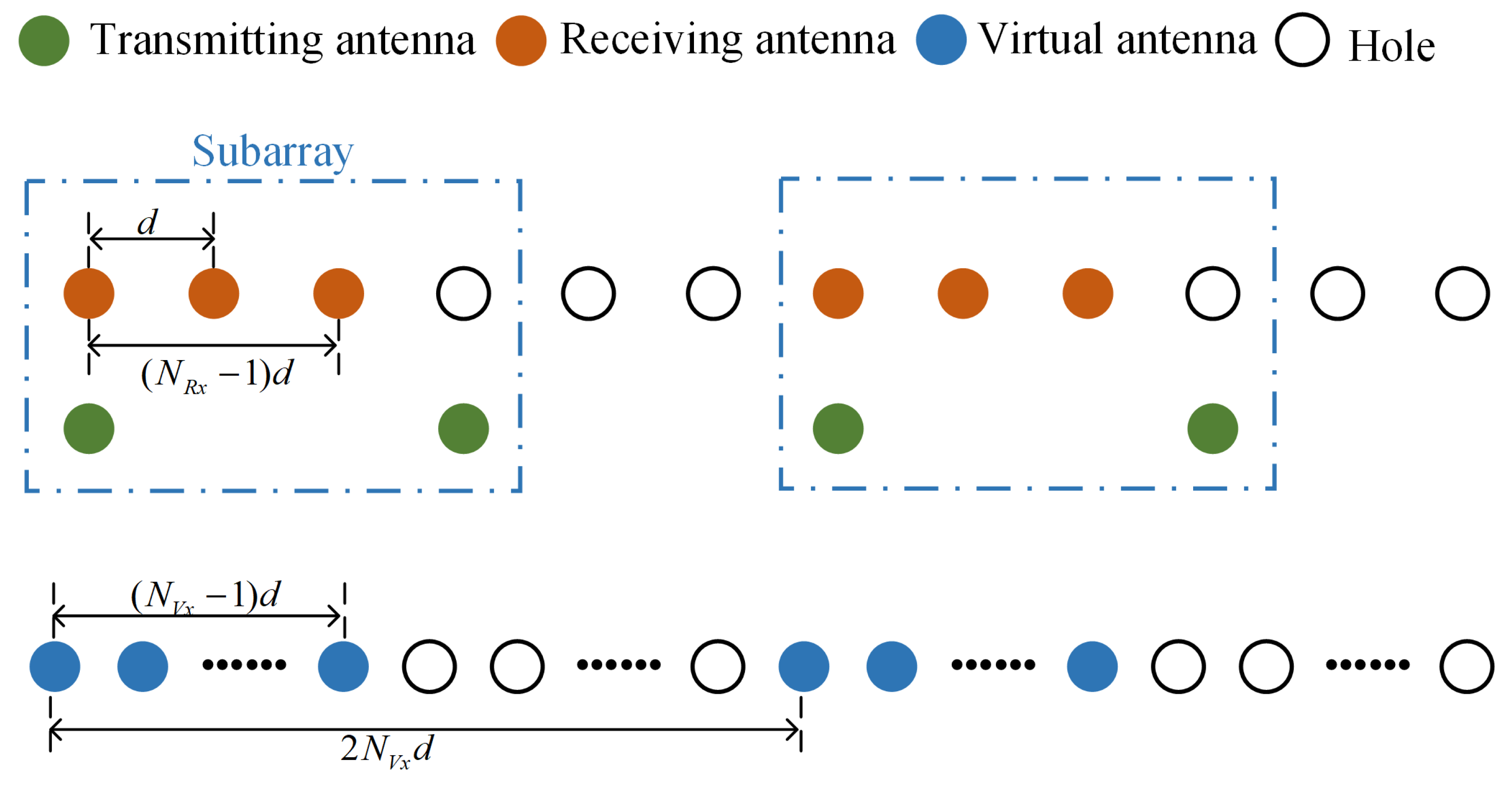
2.1. Sparse Array
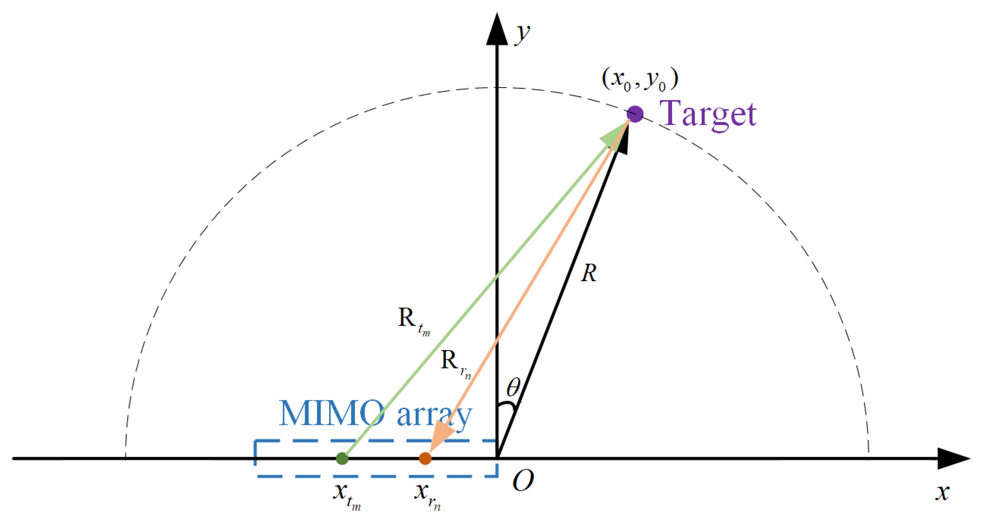
2.2. Array Imaging
3. Sparse Reconstruction Issues and Solving
3.1. Optimization Problem Expression
3.2. Implementation Using ADMM
| Algorithm 1 Sparse reconstruction algorithm. |
|
4. Results
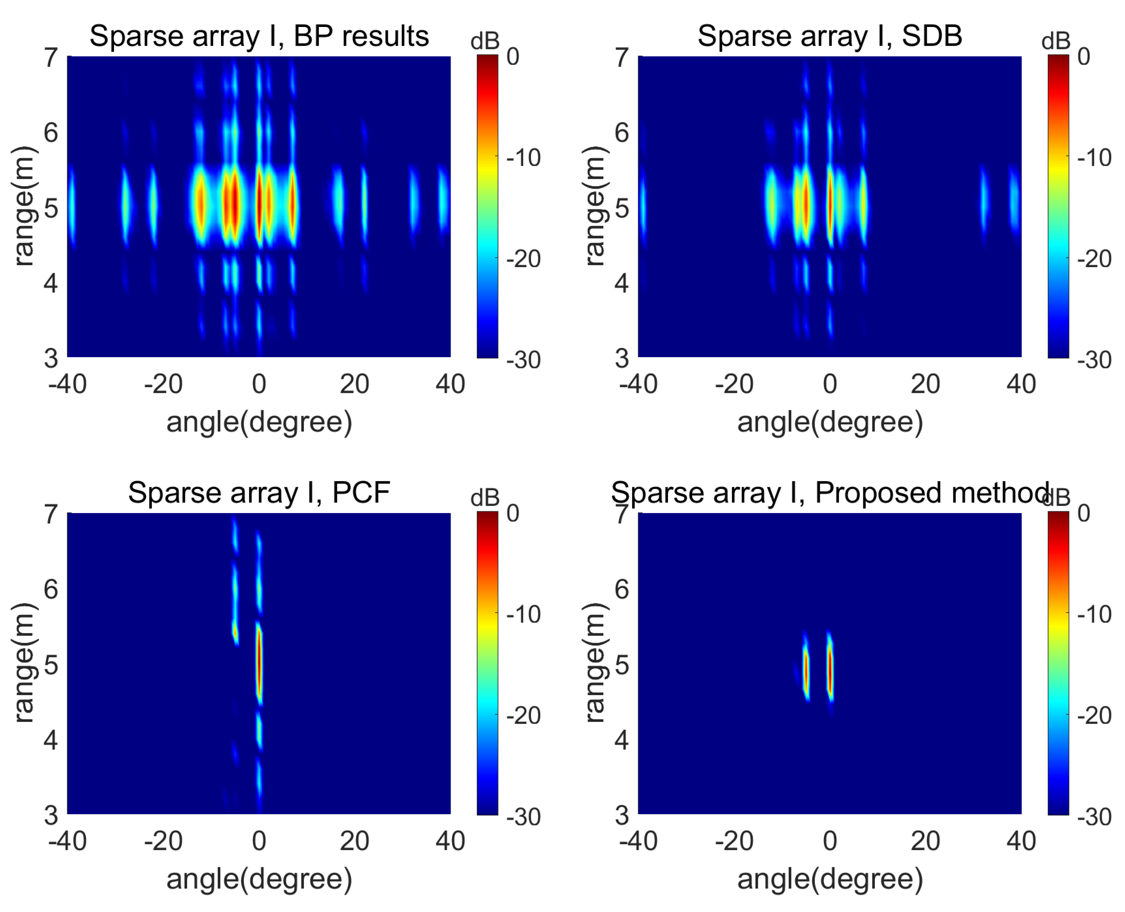
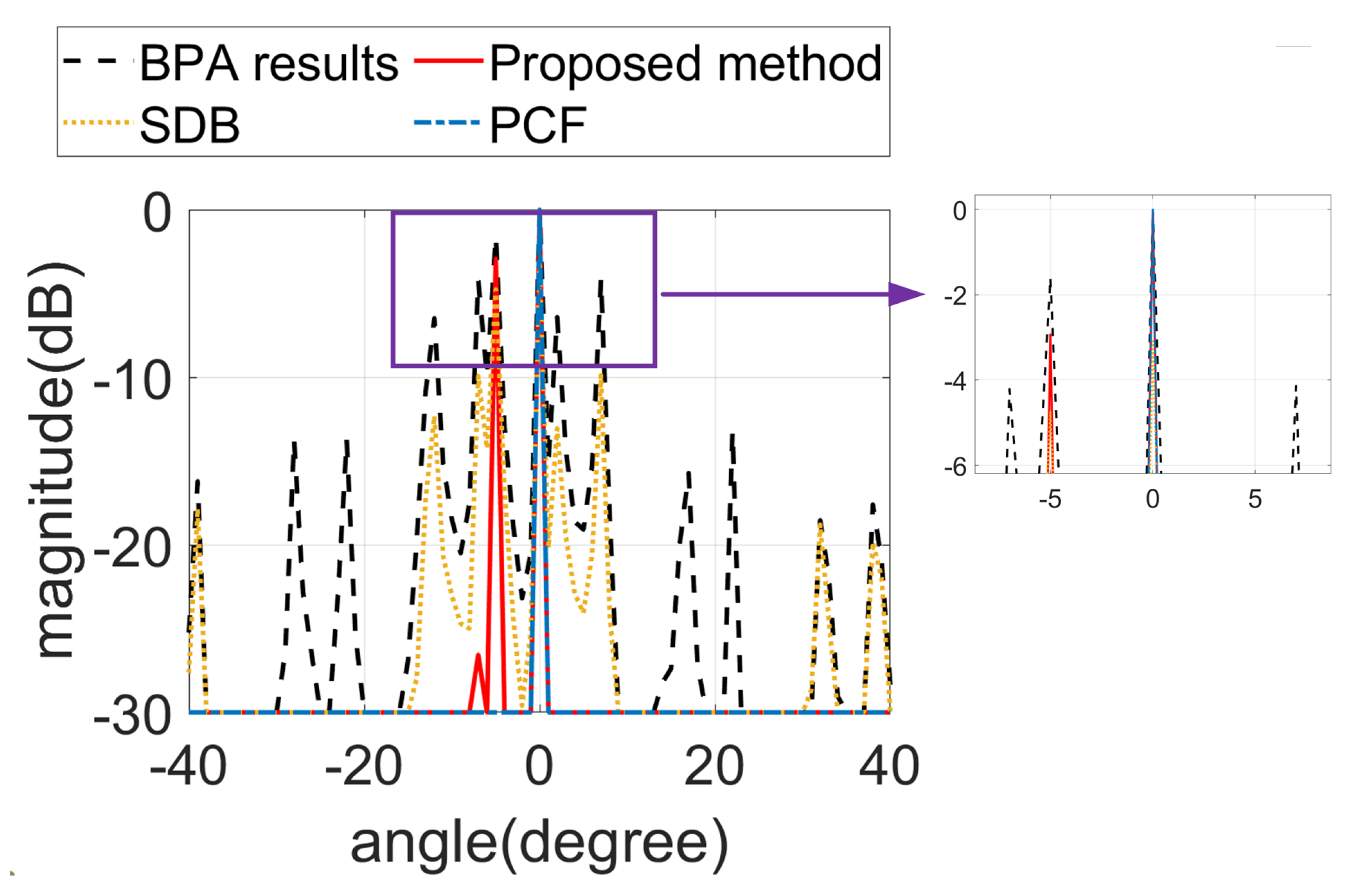
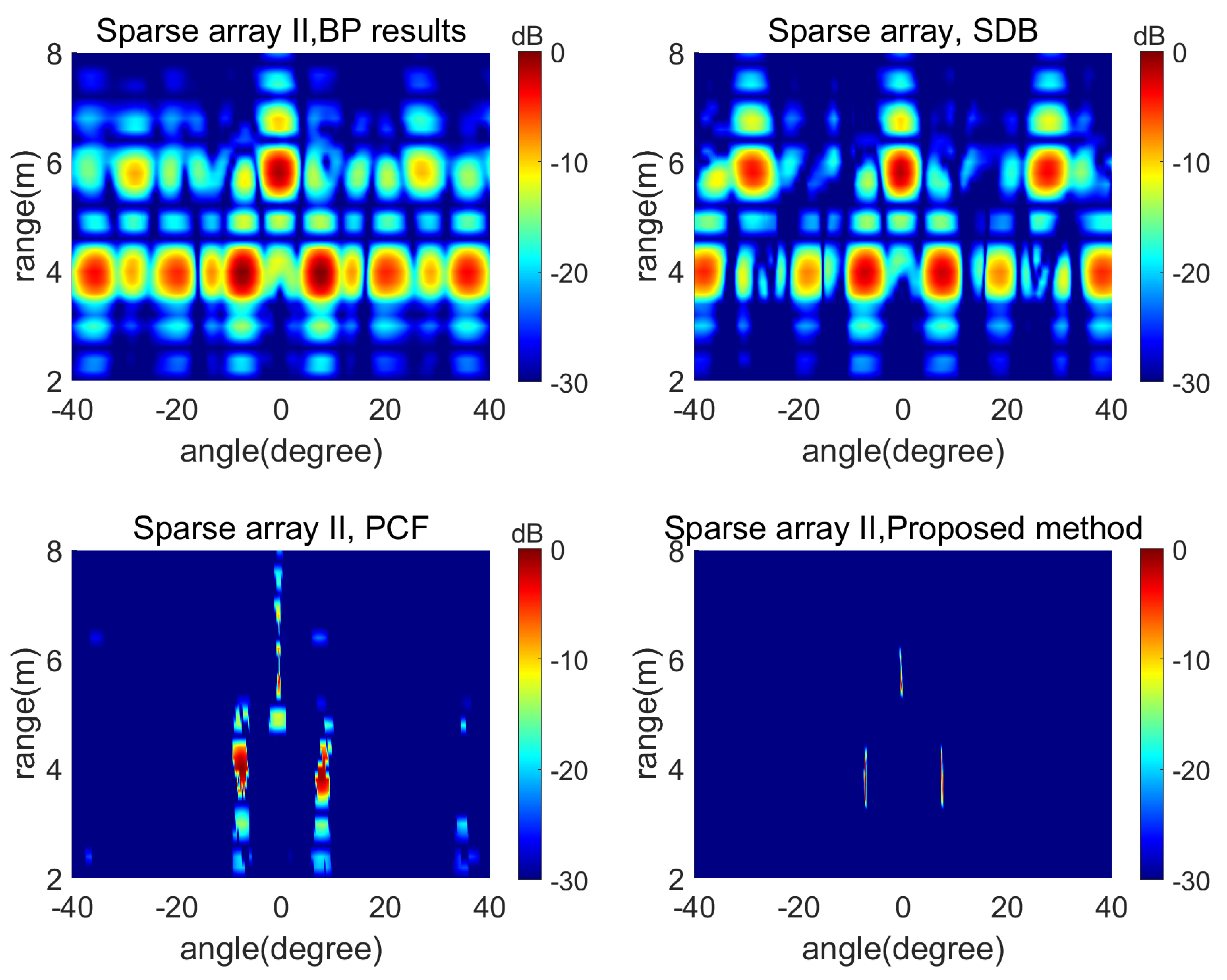
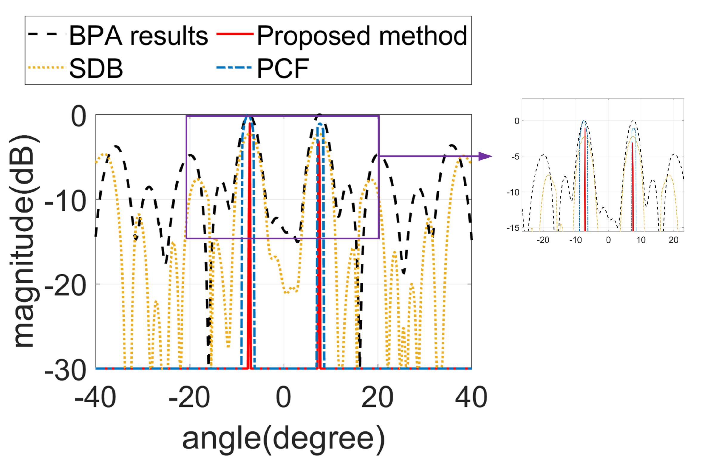
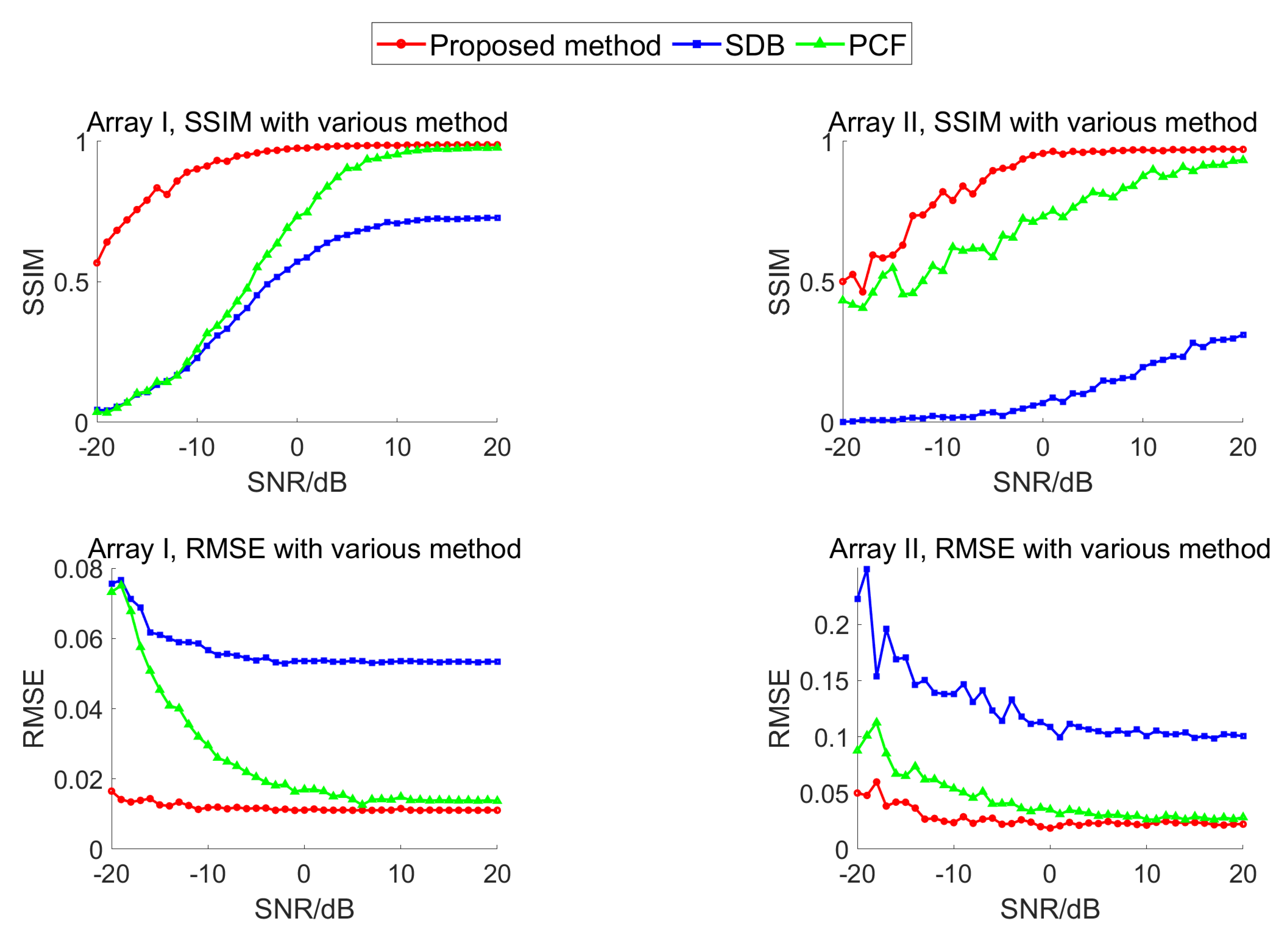
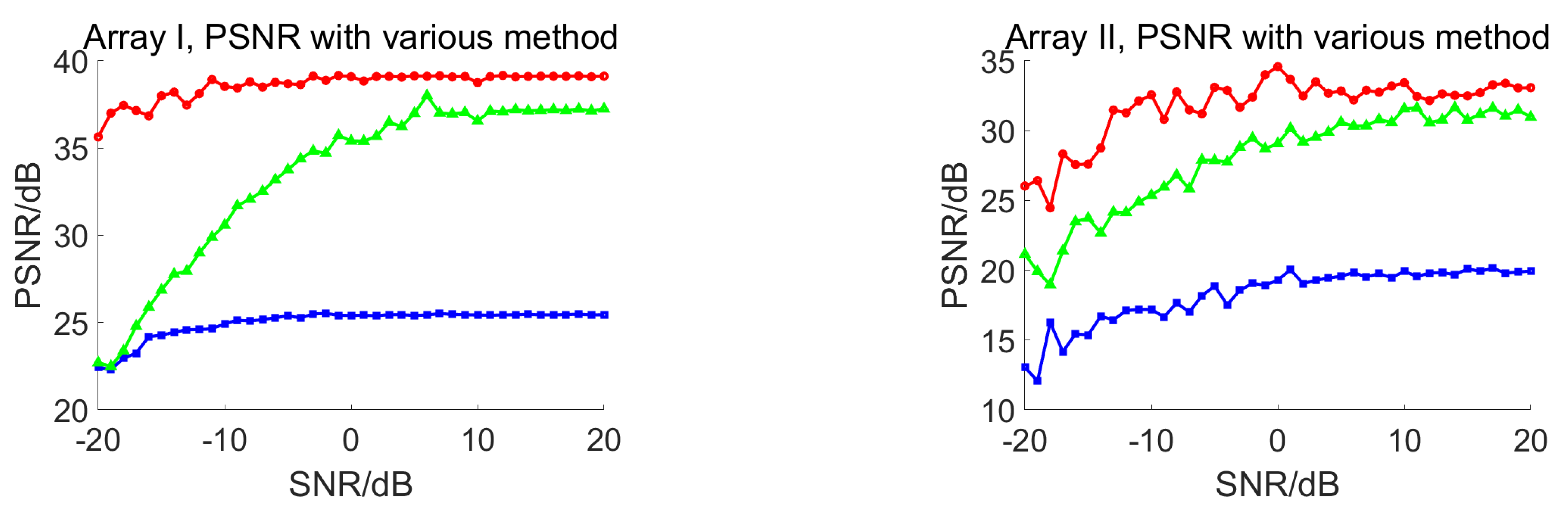
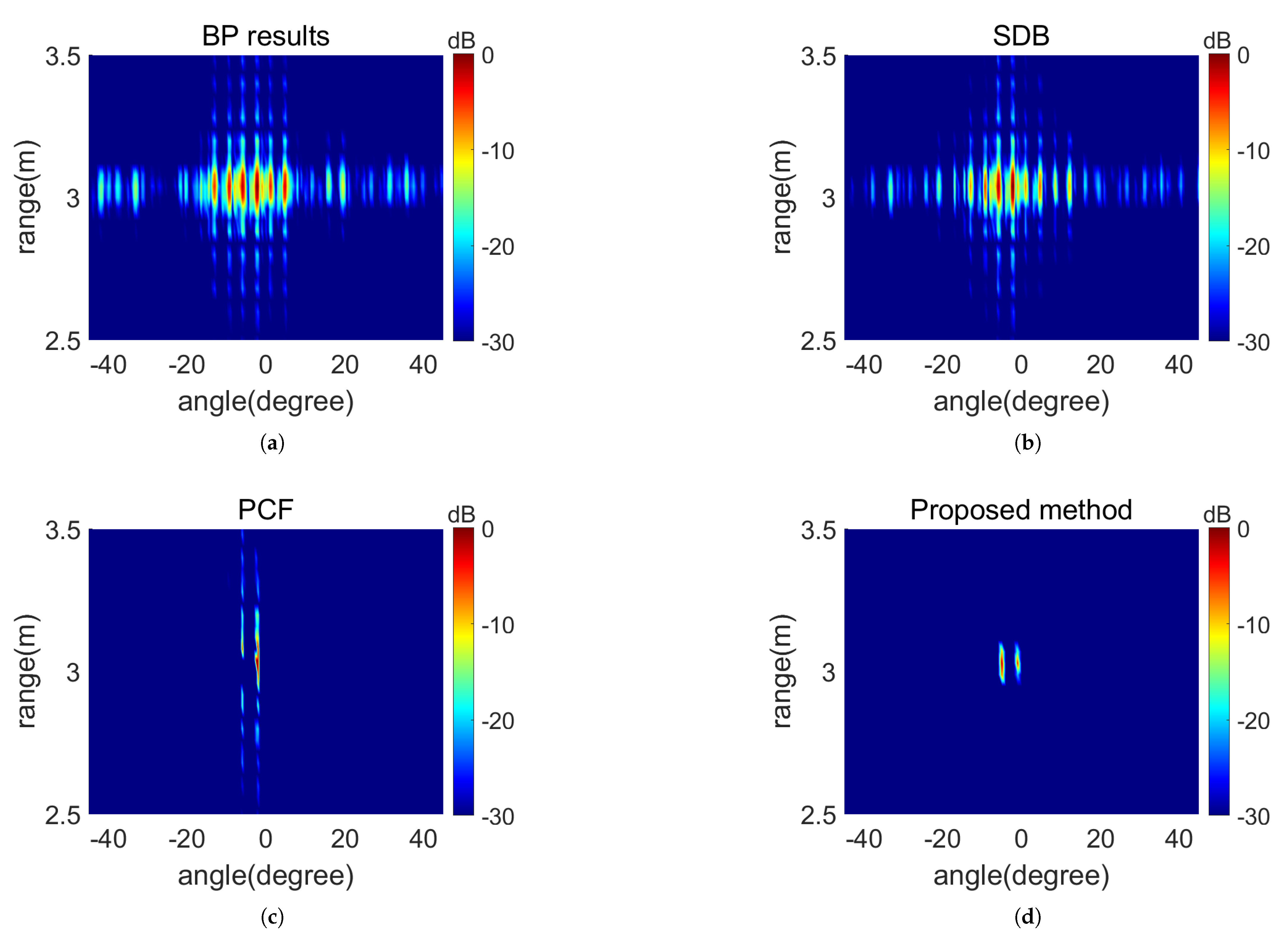
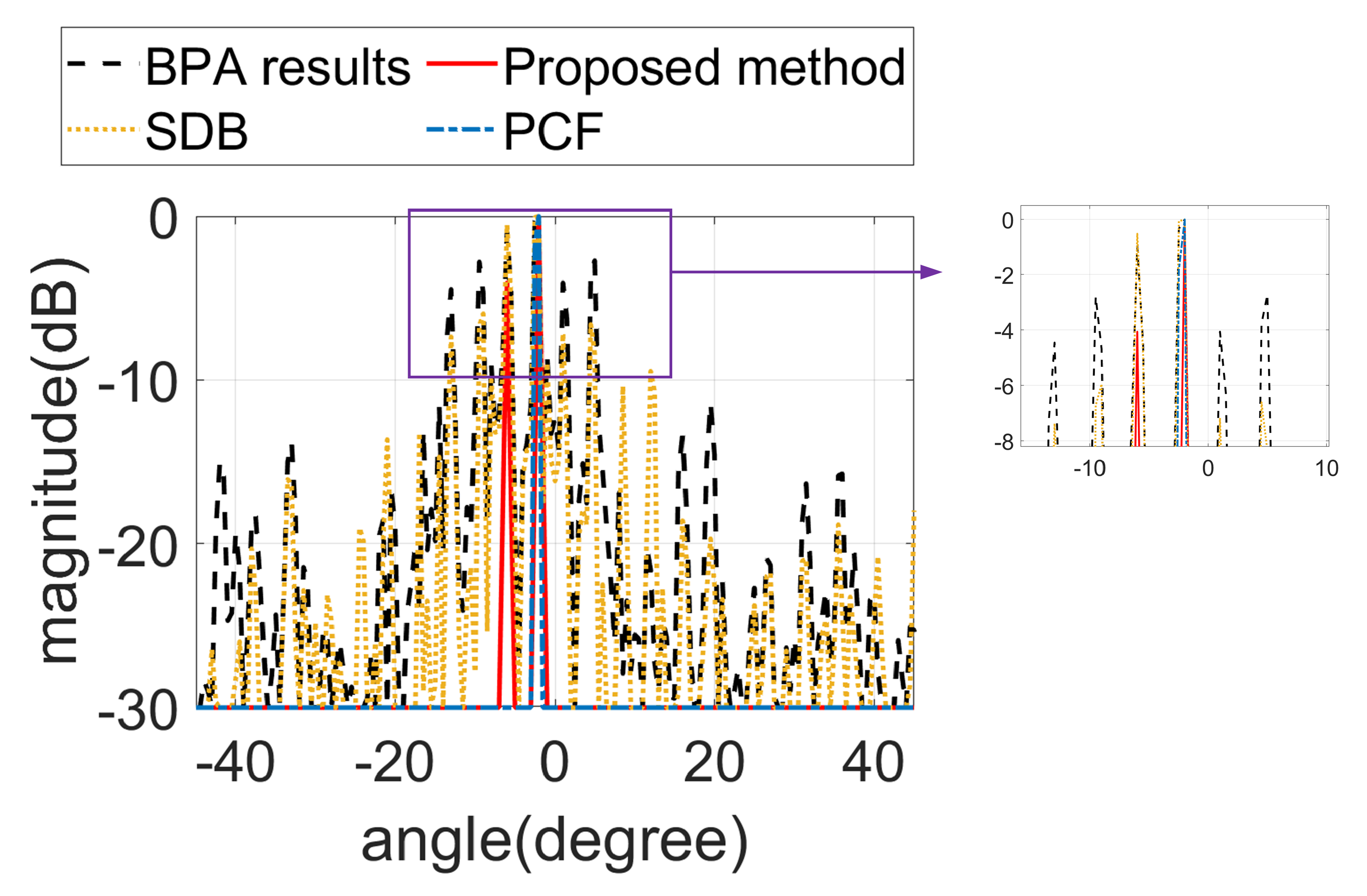
4.1. Simulation Results
4.2. Experimental Results
4.3. Analysis of Computational Speed
5. Conclusions
Author Contributions
Funding
Data Availability Statement
Conflicts of Interest
References
- Chen, D.; Nanzer, J.A. Privacy Preserving Contraband Detection Using a Millimeter-Wave Dynamic Antenna Array. IEEE Microw. Wireless Technol. Lett. 2023, 33, 915–918. [Google Scholar] [CrossRef]
- Bono, F.M.; Polinelli, A.; Radicioni, L.; Benedetti, L.; Castelli-Dezza, F.; Cinquemani, S.; Belloli, M. Wireless Accelerometer Architecture for Bridge SHM: From Sensor Design to System Deployment. Future Internet 2025, 17, 29. [Google Scholar] [CrossRef]
- Guo, T.; Wang, Y.; Xu, L.; Mei, M.; Shi, J.; Dong, L.; Xu, Y.; Huang, C. Joint communication and sensing design for multihop RIS-aided communication systems in underground coal mines. IEEE Internet Things J. 2023, 10, 19533–19544. [Google Scholar] [CrossRef]
- Shen, Z.; Nunez-Yanez, J.; Dahnoun, N. Advanced millimeter-wave radar system for real-time multiple-human tracking and fall detection. Sensors 2024, 24, 3660. [Google Scholar] [CrossRef]
- Chen, X.; Yang, Q.; Wang, H.; Zeng, Y.; Deng, B. Adaptive ADMM based high-quality fast imaging algorithm for short-range MMW MIMO-SAR systems. IEEE Trans. Antennas Propag. 2023, 71, 8925–8935. [Google Scholar] [CrossRef]
- Song, T.; Yao, X.; Wang, L.; Wang, Y.; Sun, G. Fast Factorized Kirchhoff Migration Algorithm for Near-Field Radar Imaging with Sparse MIMO Arrays. IEEE Trans. Geosci. Remote Sens. 2024, 62, 1–14. [Google Scholar] [CrossRef]
- Syeda, R.Z.; Adela, B.B.; van Beurden, M.C.; Zeijl, P.T.M.v.; Smolders, A.B. Design of a mm-wave MIMO radar demonstrator with an array of FMCW radar chips with on-chip antennas. In Proceedings of the 16th European Radar Conference, Paris, France, 2–4 October 2019; pp. 33–36. [Google Scholar]
- Qu, H.; Zhai, L. Optimization of Sparse synthesis aperture imaging array on hexagonal grids with difference basis. In Proceedings of the 2014 IEEE International Conference on Signal Processing, Communications and Computing, Guilin, China, 5–8 August 2014; pp. 544–548. [Google Scholar]
- Merlo, J.M.; Wagner, S.; Lancaster, J.; Nanzer, J.A. Fully Wireless Coherent Distributed Phased Array System for Networked Radar Applications. IEEE Microw. Wirel. Technol. Lett. 2024, 34, 837–840. [Google Scholar] [CrossRef]
- Bhattacharyya, A.; Merlo, J.M.; Mghabghab, S.R.; Schlegel, A.; Nanzer, J.A. Multiobjective Distributed Array Beamforming in the Near Field Using Wireless Syntonization. IEEE Microw. Wirel. Technol. Lett. 2023, 33, 775–778. [Google Scholar] [CrossRef]
- Zhu, J.; Lei, P.; Wang, J.; Zhang, Y.; Yuan, C. Grating Lobe Suppression and Angle Estimation Based on Virtual Antennas Filling in Sparse Array. IEEE Antennas Wirel. Propag. Lett. 2023, 22, 502–506. [Google Scholar] [CrossRef]
- Goffer, A.P.; Kam, M.; Herczfeld, P.R. Design of phased arrays in terms of random subarrays. IEEE Trans. Antennas Propag. 1994, 42, 820–826. [Google Scholar] [CrossRef]
- Alshammary, A.; Weiss, S.; Almorqi, S. Grating lobe suppression in rotationally tiled arrays. In Proceedings of the 11th European Conference on Antennas and Propagation, Paris, France, 19–24 March 2017; pp. 1158–1161. [Google Scholar]
- Feng, B.K.; Jenn, D.C. Two-way pattern grating lobe control for distributed digital subarray antennas. IEEE Trans. Antennas Propag. 2015, 63, 4375–4383. [Google Scholar] [CrossRef]
- Feng, B.K.; Jenn, D.C. Grating lobe suppression for distributed digital subarrays using virtual filling. IEEE Antennas Wirel. Propag. Lett. 2013, 12, 1323–1326. [Google Scholar] [CrossRef]
- Lv, J.; Song, Y.; Li, Z.; Wu, J. A Grating Lobe Suppression Approach for Distributed Mimo Array Radar Backprojection Algorithm. In Proceedings of the IEEE International Geoscience and Remote Sensing Symposium (IGARSS), Kuala Lumpur, Malaysia, 17–22 July 2022; pp. 3444–3447. [Google Scholar]
- Han, K.; Hong, S. High-resolution phased-subarray MIMO radar with grating lobe cancellation technique. IEEE Trans. Microw. Theory Techn. 2022, 70, 2775–2785. [Google Scholar] [CrossRef]
- Zhu, R.; Zhou, J.; Jiang, G.; Cheng, B.; Fu, Q. Grating lobe suppression in near range MIMO array imaging using zero migration. IEEE Trans. Microw. Theory Techn. 2020, 68, 387–397. [Google Scholar] [CrossRef]
- Bazzi, A.; Slock, D.T.M.; Meilhac, L.; Panneerselvan, S. A comparative study of sparse recovery and compressed sensing algorithms with application to AoA estimation. In Proceedings of the 2016 IEEE 17th International Workshop on Signal Processing Advances in Wireless Communications, Edinburgh, UK, 3–6 July 2016; pp. 1–5. [Google Scholar]
- Mwisomba, C.; Abdalla, A.T.; Amour, I.; Mkemwa, F.; Maiseli, B. Fast sparse image reconstruction method in through-the-wall radars using limited memory Broyden–Fletcher–Goldfarb–Shanno algorithm. Int. J. Microw. Wirel. Technol. 2022, 14, 739–749. [Google Scholar] [CrossRef]
- Hashempour, H.R. A fast ADMM-based approach for high resolution ISAR imaging. Electron. Lett. 2020, 56, 954–957. [Google Scholar] [CrossRef]
- Dedai, M.D.; Jenkins, W.K. Convolution back-projection image reconstruction for Spotlight Mode Synthetic Aperture radar. IEEE Trans. Image Process. 1992, 1, 505–516. [Google Scholar]
- Wang, Y.; Wang, J.; He, G.; Song, T.; Zhu, J.; Zhang, C.; He, X. Enhancing 3D SAR Imaging: A Near-Field Back Projection Algorithm for Addressing Geometric Distortion. In Proceedings of the IGARSS 2024 IEEE International Geoscience and Remote Sensing Symposium, Athens, Greece, 7–12 July 2024; pp. 9648–9652. [Google Scholar]
- He, J.; Wang, J.; Yang, B.; Zhao, K.; Bao, Y.; Wang, Y.; Geng, X. Near-Field Radar Imaging Using MMIC-Based Large-Aperture Array. IEEE Sens. J. 2024, 24, 30863–30874. [Google Scholar] [CrossRef]
- Zou, H. The Adaptive Lasso and Its Oracle Properties. J. Am. Stat. Assoc. 2006, 101, 1418–1429. [Google Scholar] [CrossRef]
- Boyd, S. Distributed optimization and statistical learning via the alter-ating direction method of multipliers. Found. Trends Mach. Learn. 2010, 3, 1–122. [Google Scholar] [CrossRef]
- Kim, S.-J.; Koh, K.; Lustig, M.; Boyd, S.; Gorinevsky, D. An interior-point method for large-scale ℓ1-regularized least squares. IEEE J. Sel. Topics Signal Process. 2007, 1, 606–617. [Google Scholar] [CrossRef]
- Xu, L.; Sun, S.; We, R.; Ren, D.; Li, J. Generalized Optimization of Sparse Antenna Arrays for High-Resolution Automotive Radar Imaging. In Proceedings of the 2023 57th Asilomar Conference on Signals, Systems, and Computers, Pacific Grove, CA, USA, 29 October–1 November 2023; pp. 1215–1219. [Google Scholar]
- Haji, S.H.; Abdulazeez, A.M. Comparison of optimization techniques based on gradient descent algorithm: A review. PalArch’s J. Archaeol. Egypt/Egyptol. 2021, 18, 2715–2743. [Google Scholar]
- Parikh, N.; Boyd, S. Proximal algorithms. Found. Trends Optim. 2014, 1, 127–239. [Google Scholar] [CrossRef]


| Parameter | Value |
|---|---|
| Center frequency | 75 GHz |
| Bandwidth | 1.75 GHz |
| Sweep frequency time | 30 µs |
| Sampling frequency | 20 MHz |
| Pulse period | 45 µs |
| µ in (18) | 1 |
| Image region | [0, 10 m] × [−45°, 45°] |
| Image size | 100 × 91 |
| Algorithm | IE | IC |
|---|---|---|
| BP results | 2.35 | 2.06 |
| SDB | 1.86 | 2.43 |
| PCF | 0.25 | 6.26 |
| Proposed method | 0.09 | 7.74 |
| Algorithm | Runtime (s) |
|---|---|
| Gradient descent | 29.5 |
| PPA | 20.1 |
| ADMM | 2.3 |
| SDB | 0.29 |
| PCF | 0.35 |
Disclaimer/Publisher’s Note: The statements, opinions and data contained in all publications are solely those of the individual author(s) and contributor(s) and not of MDPI and/or the editor(s). MDPI and/or the editor(s) disclaim responsibility for any injury to people or property resulting from any ideas, methods, instructions or products referred to in the content. |
© 2025 by the authors. Licensee MDPI, Basel, Switzerland. This article is an open access article distributed under the terms and conditions of the Creative Commons Attribution (CC BY) license (https://creativecommons.org/licenses/by/4.0/).
Share and Cite
Wang, Y.; Wang, J.; Chen, P.; He, G.; He, J. A Grating Lobe Near-Field Image Enhancement Method: Sparse Reconstruction Based on Alternating Direction Method of Multipliers. Electronics 2025, 14, 1514. https://doi.org/10.3390/electronics14081514
Wang Y, Wang J, Chen P, He G, He J. A Grating Lobe Near-Field Image Enhancement Method: Sparse Reconstruction Based on Alternating Direction Method of Multipliers. Electronics. 2025; 14(8):1514. https://doi.org/10.3390/electronics14081514
Chicago/Turabian StyleWang, Yuanhao, Jun Wang, Penghui Chen, Guidong He, and Jiacheng He. 2025. "A Grating Lobe Near-Field Image Enhancement Method: Sparse Reconstruction Based on Alternating Direction Method of Multipliers" Electronics 14, no. 8: 1514. https://doi.org/10.3390/electronics14081514
APA StyleWang, Y., Wang, J., Chen, P., He, G., & He, J. (2025). A Grating Lobe Near-Field Image Enhancement Method: Sparse Reconstruction Based on Alternating Direction Method of Multipliers. Electronics, 14(8), 1514. https://doi.org/10.3390/electronics14081514