
A Novel Fault Diagnosis and Accurate Localization Method for a Power System Based on GraphSAGE Algorithm


Abstract
1. Introduction
2. Graph Neural Network
2.1. Graph Convolutional Neural Network
2.2. GraphSAGE Algorithm
3. Database Construction
3.1. Fault Simulation in Power Systems
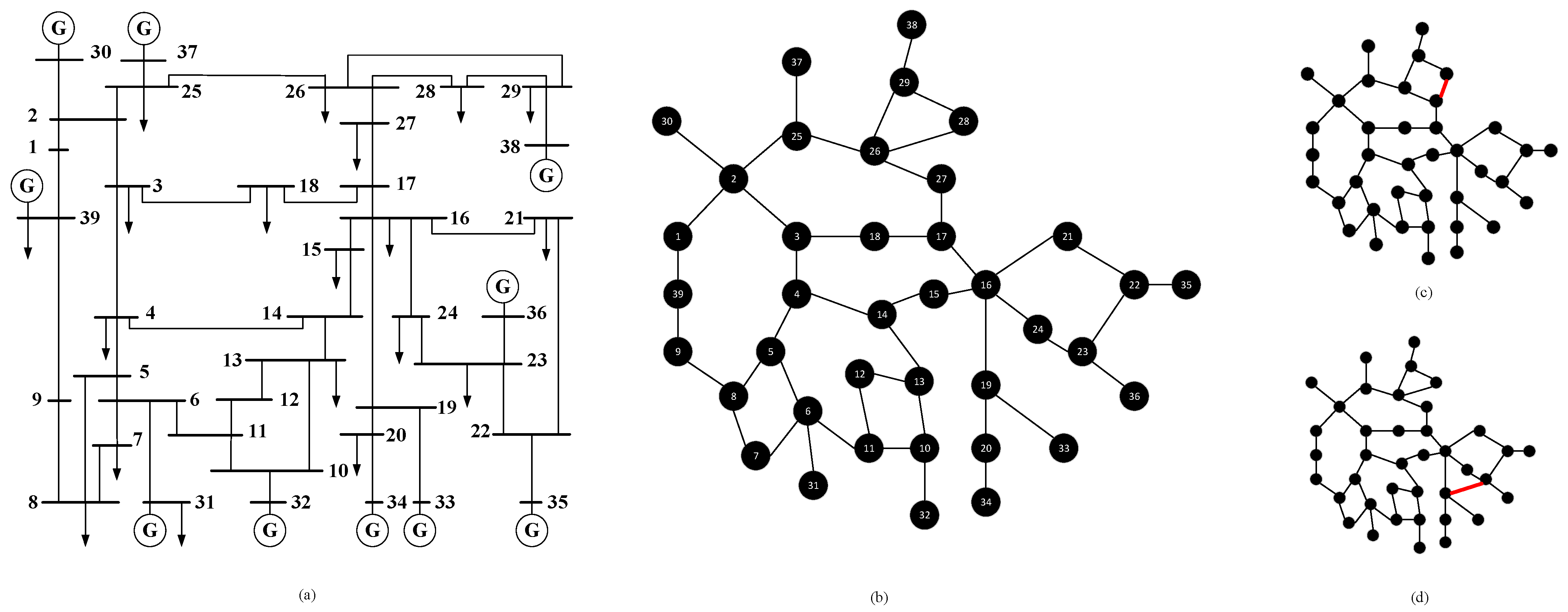
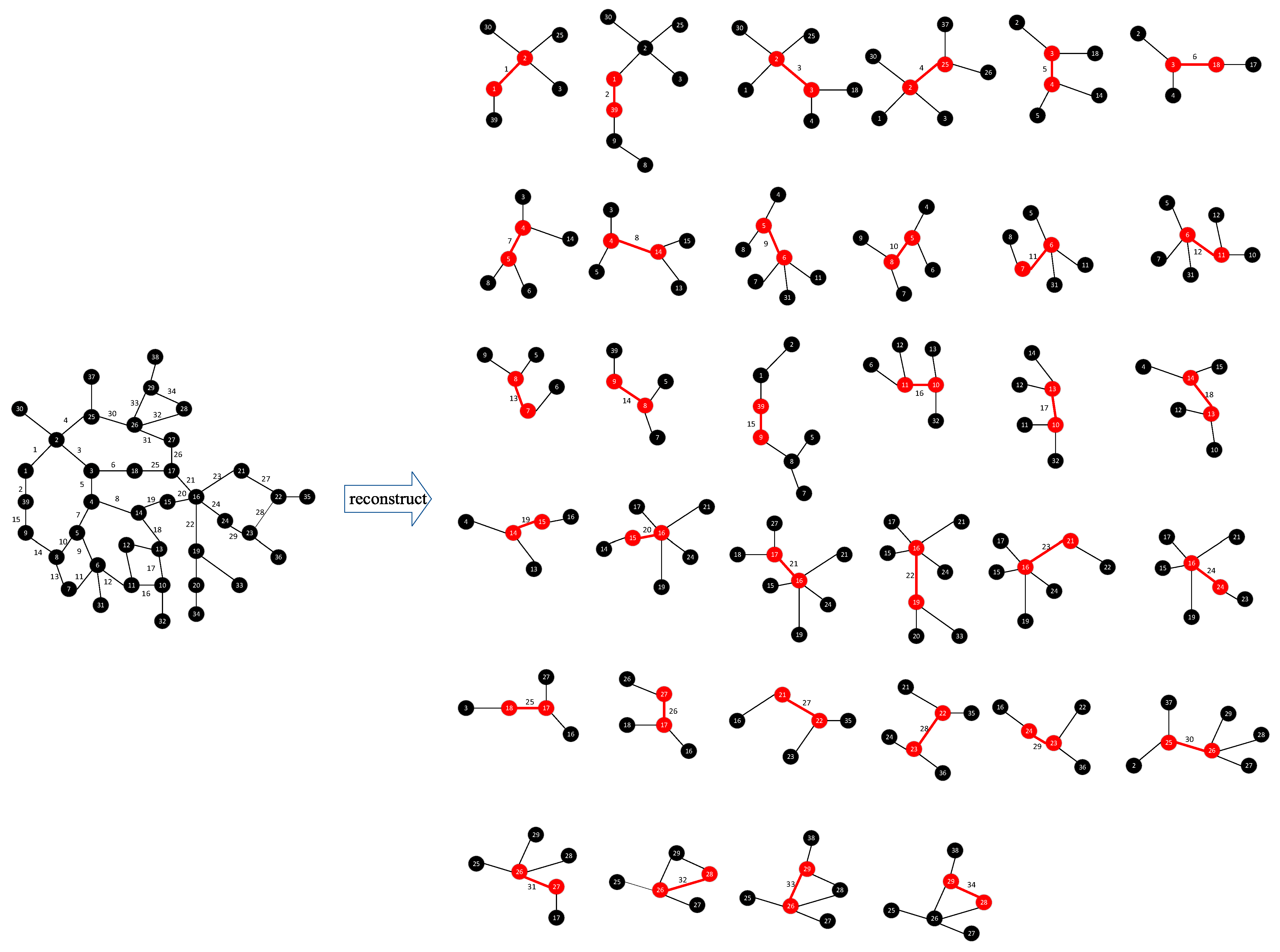
3.2. Graph Structure Construction
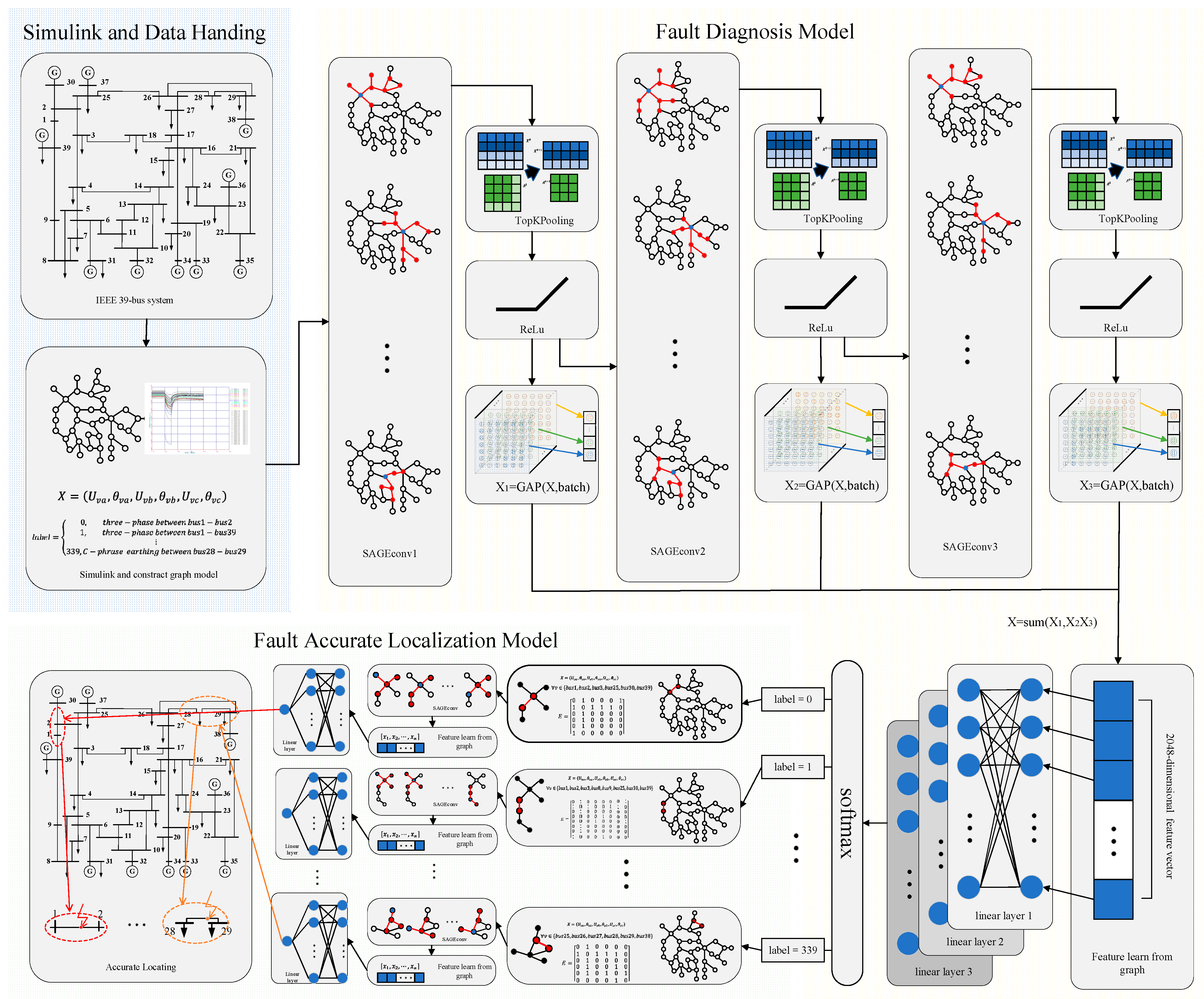
4. Fault Diagnosis and Accurate Localization Model of Power System Based on GraphSAGE Algorithm
5. Validation Experiments
5.1. Diagnosis Model Validation
5.2. Accurate Localization Model Validation
6. Conclusions
- (1)
- While some studies have used GCN, GAT, classical deep learning (CNN), and machine learning (Bayesian network) methods to address fault type classification and fault interval localization in power grids. Few studies have also established an AI-based model for accurate fault localization. This article introduces an innovative approach by using GraphSAGE to build an accurate fault localization model, leveraging its inductive learning capability and fully utilizing topological information to realize accurate fault localization;
- (2)
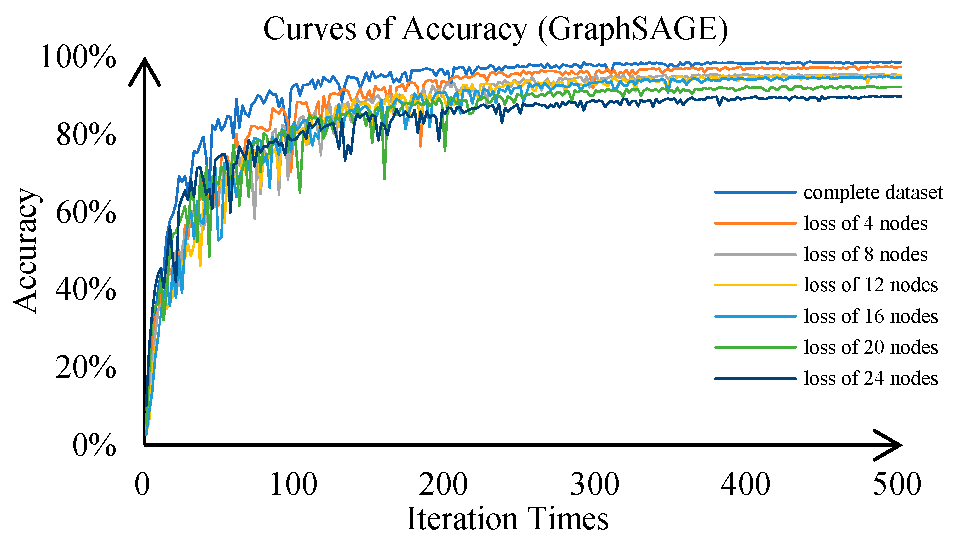
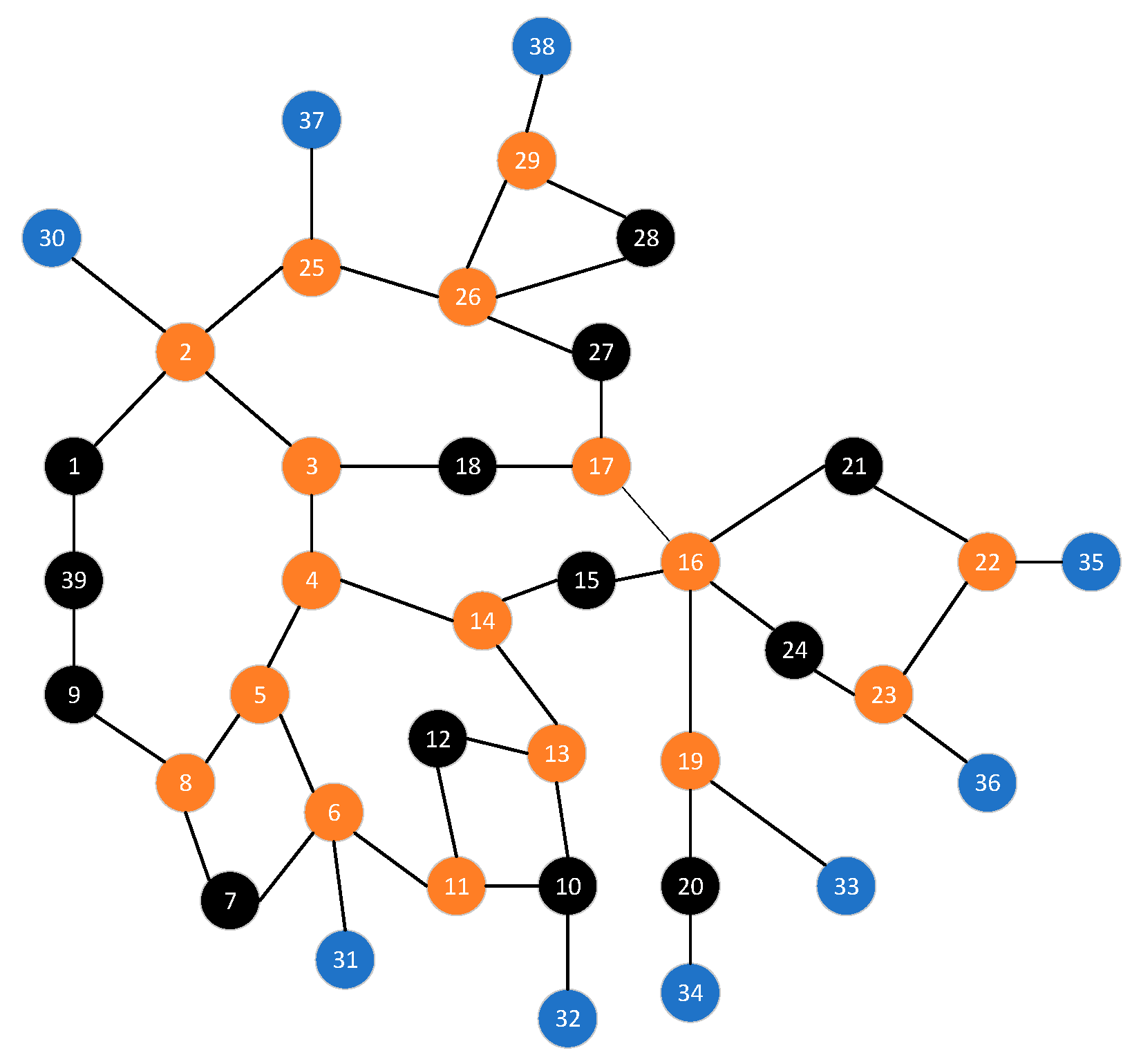
- Extensive validation data demonstrate that the higher the degree of a node, the more effectively it can learn features from neighboring nodes. This property allows for the identification of key nodes when processing large-scale power grid data, thereby reducing the complexity of the model while maintaining accuracy;
- (3)
- In simulations involving topology changes in the power grid, GraphSAGE consistently outperforms GCN and GAT, with an accuracy improvement of about 3% and 2%. This demonstrates its strong adaptability to topology variations and excellent practical applicability;
- (4)
- In the accurate localization model, the random sampling characteristic and inductive learning capability of the GraphSAGE algorithm can achieve significantly higher localization accuracy compared to GAT and GCN;
- (5)
- When the line length does not exceed 7.5 km, this method offers certain advantages over the traveling wave method. Moreover, this method offers greater economic practicality compared to the traveling wave method.
Author Contributions
Funding
Data Availability Statement
Conflicts of Interest
References
- Tong, H.; Qiu, R.C.; Zhang, D.; Yang, H.; Ding, Q.; Shi, X. Detection and classification of transmission line transient faults based on graph convolutional neural network. CSEE J. Power Energy Syst. 2021, 7, 456–471. [Google Scholar]
- Meghwani, A.; Srivastava, S.C.; Chakrabarti, S. Local measurement-based technique for estimating fault location in multi-source DC microgrids. IET Gener. Transm. Distrib. 2018, 12, 3305–3313. [Google Scholar] [CrossRef]
- Nougain, V.; Mishra, S.; Nag, S.S.; Lekić, A. Fault Location Algorithm for Multi-Terminal Radial Medium Voltage DC Microgrid. IEEE Trans. Power Deliv. 2023, 38, 4476–4488. [Google Scholar] [CrossRef]
- Han, H.; Zheng, X.L.; Su, M.; Sun, Y.; Liu, Z.J.; Liu, H.Y. A Fast Fault Diagnosis Scheme for Ring Bus DC Microgrids with Fewer Sensors. IEEE Trans. Power Deliv. 2024, 39, 283–295. [Google Scholar] [CrossRef]
- Ahmed, M.S.; Vokony, I.; Muhammad, A.K.; Muhammad, W.; Amgad, N.A.A. Power system stability in the Era of energy Transition: Importance Opportunities, Challenges, and future directions. Energy Convers. Manag. X 2024, 24. [Google Scholar] [CrossRef]
- Yu, J.J.Q.; Hou, Y.; Lam, A.Y.S.; Li, V.O.K. Intelligent Fault Detection Scheme for Microgrids with Wavelet-Based Deep Neural Networks. IEEE Trans. Smart Grid 2019, 10, 1694–1703. [Google Scholar] [CrossRef]
- Liao, W.; Yang, D.; Wang, Y.; Ren, X. Fault diagnosis of power transformers using graph convolutional network. CSEE J. Power Energy Syst. 2021, 7, 241–249. [Google Scholar]
- Chen, K.; Hu, J.; Zhang, Y.; Yu, Z.; He, J. Fault Location in Power Distribution Systems via Deep Graph Convolutional Networks. IEEE J. Sel. Areas Commun. 2021, 38, 119–131. [Google Scholar] [CrossRef]
- Li, P.; Liu, X.Y.; Yuan, Z.Y.; Chen, W.; Yu, L.; Xu, Q. Precise Fault Location Method of Traveling Wave in Distribution Grid Based on Multiple Measuring Point. In Proceedings of the 2020 IEEE 4th Conference on Energy Internet and Energy System Integration (EI2), Wuhan, China, 30 October–1 November 2020; pp. 1867–1872. [Google Scholar]
- Nityananda, G.; Pravati, N.; Ranjan, K.M.; Sairam, M.; Aymen, F.; Habib, K.; Lukas, P.; Mohammad, K. Wavelet-Based ensembled intelligent technique for a better quality of fault detection and classification in AC microgrids. Energy Convers. Manag. 2024, 24, 100813. [Google Scholar]
- Bhargav, R.; Bhalja, B.R.; Gupta, C.P. Novel fault detection and localization algorithm for low-voltage DC microgrid. IEEE Trans. Ind. Inform. 2019, 16, 4498–4511. [Google Scholar] [CrossRef]
- Bayati, N.; Balouji, E.; Baghaee, H.R.; Hajizadeh, A.; Soltani, M.; Lin, Z.; Savaghebi, M. Locating high-impedance faults in DC microgrid clusters using support vector machines. Appl. Energy 2022, 308, 118338. [Google Scholar] [CrossRef]
- Nikolaos, S.; Jesus, L.; Bertrand, R. Fault diagnosis in low voltage smart distribution grids using gradient boosting trees. Electr. Power Syst. Res. 2020, 182, 106254. [Google Scholar]
- Zheng, C.; Zhu, G.; Qin, F.; Lan, J.; Li, S. Distribution Network Fault Segment Location Algorithm Based on Bayesian Estimation in Intelligent Distributed Control Mode. In Proceedings of the 2020 Asia Energy and Electrical Engineering Symposium (AEEES), Chengdu, China, 19 June 2020; pp. 592–596. [Google Scholar]
- Govind, V.; Sumika, C.; Mert, S.; Justyna, H.S.; Radoslaw, Z.; Patrick, D.; Rajesh, K. Advancing Machine Fault Diagnosis: A Detailed Examination of Convolutional Neural Networks. Meas. Sci. Technol. 2024, 36, 022001. Available online: https://iopscience.iop.org/article/10.1088/1361-6501/ada178 (accessed on 20 January 2025).
- Meng, Z.; Du, W.; Wang, H. Distribution network fault area location based on deep convolution neural network with transfer learning. South. Power Syst. Technol. 2019, 13, 25–33. (In Chinese) [Google Scholar]
- Liao, W.; Bak-Jensen, B.; Pillai, J.R.; Wang, Y.; Wang, Y. A review of graph neural networks and their applications in power systems. J. Mod. Power Syst. Clean Energy 2022, 10, 345–360. [Google Scholar] [CrossRef]
- Ling, W.; Gao, S.; Wei, X.; Wu, X.; Shi, J.; Lei, J. GCN for Identifying Critical Branches Based on Unlabeled Power Outage Data. IEEE Trans. Power Syst. 2024, 39, 7441–7444. [Google Scholar] [CrossRef]
- Xia, S.W.; Zhang, C.H.; Li, Y.H.; Li, G.Y.; Ma, L.L.; Zhou, N. GCN-LSTM Based Transient Angle Stability Assessment Method for Future Power Systems Considering Spatial-Temporal Disturbance Response Characteristics. Prot. Control Mod. Power Syst. 2024, 9, 108–121. [Google Scholar] [CrossRef]
- Hu, J.; Wang, Q.; Ye, Y.; Wu, Z.; Tang, Y. A High Temporal-Spatial Resolution Power System State Estimation Method for Online DSA. IEEE Trans. Power Syst. 2024, 39, 877–889. [Google Scholar] [CrossRef]
- Vincent, E.; Korki, M.; Seyedmahmoudian, M.; Stojcevski, A.; Mekhilef, S. Reinforcement Learning-Empowered Graph Convolutional Network Framework for Data Integrity Attack Detection in Cyber-Physical Systems. CSEE J. Power Energy Syst. 2024, 10, 797–806. [Google Scholar]
- Yang, H.; Li, X.W.; ZhiJian, S.; Zhang, X. Accident prediction of power distribution network based on graph neural network. Comput. Syst. Appl. 2020, 29, 131–135. (In Chinese) [Google Scholar]
- Zhai, Y.; Wang, Q.; Yang, X.; Zhao, Z.; Zhao, W. Multi-Fitting Detection on Transmission Line Based on Cascade Reasoning Graph Network. IEEE Trans. Power Deliv. 2022, 37, 4858–4868. [Google Scholar] [CrossRef]
- Azizi, S.; Sanaye-Pasand, M.; Abedini, M.; Hasani, A. A traveling-wave-based methodology for wide-area fault location in multiterminal DC systems. IEEE Trans. Power Deliv. 2014, 29, 2552–2560. [Google Scholar] [CrossRef]
- Dhar, S.; Patnaik, R.K.; Dash, P.K. Fault detection and location of photovoltaic based DC microgrid using differential protection strategy. IEEE Trans. Smart Grid 2017, 9, 4303–4312. [Google Scholar] [CrossRef]
- Hamilton, W.L.; Ying, R.; Leskovec, J. Inductive representation learning on large graphs. In Proceedings of the 31st International Conference on Neural Information Processing Systems, Long Beach, CA, USA, 4–9 December 2017; pp. 1025–1035. [Google Scholar]
- Yin, Z.; Wang, S.; Zhao, Q. A Flexibility Scheduling Method for Distribution Network Based on Robust Graph DRL Against State Adversarial Attacks. J. Mod. Power Syst. Clean Energy 2024, 1–13. [Google Scholar]
- Zhao, Y.; Liu, J.; Liu, X.; Yuan, K.; Ren, K.; Yang, M. A Graph-based Deep Reinforcement Learning Framework for Autonomous Power Dispatch on Power Systems with Changing Topologies. In Proceedings of the 2022 IEEE Sustainable Power and Energy Conference (iSPEC), Perth, Australia, 4–7 December 2022; pp. 1–5. [Google Scholar]
- Ding, Y.; Wu, H.; Xu, Z.; Yang, H. GraphSAGE-Based Probabilistic Optimal Power Flow in Distribution System. In Proceedings of the 2023 International Conference on Power System Technology (PowerCon), Jinan, China, 21–22 September 2023; pp. 1–5. [Google Scholar]
- Lin, H.; Chen, Z.; Chen, J.; Chen, W. Transient Stability Analysis of AC-DC Hybrid Power Grid under Topology Changes Based on Deep Learning. In Proceedings of the 2022 12th International Conference on Power and Energy Systems (ICPES), Guangzhou, China, 23–25 December 2022; pp. 514–519. [Google Scholar]


| Parameter Settings | |
|---|---|
| Fault type | single-phase grounding (A-phase, B-phase, C-phase), two-phase short circuit (AB-phase, BC-phase, AC-phase), two-phase grounding (AB-phase, BC-phase, AC-phase), three-phase short circuit |
| Fault point position | 10%, 20%, …, 90% |
| Load level | 80%, 85%, …, 120% |
| Total sampling duration | 40 cycles |
| Sampling step size | 0.1 cycles |
| Fault start time | 10th cycle |
| Fault end time | 15th cycle |
| Types of sampling data | three-phase voltage amplitude three-phase voltage phase angle |
| Topological structure changes | connection relationship between bus1–bus2 changes to bus2–bus3 add connection relationship bus19–bus23 |
| Models | GraphSAGE | GCN | GAT | CNN | Bayesian Network |
|---|---|---|---|---|---|
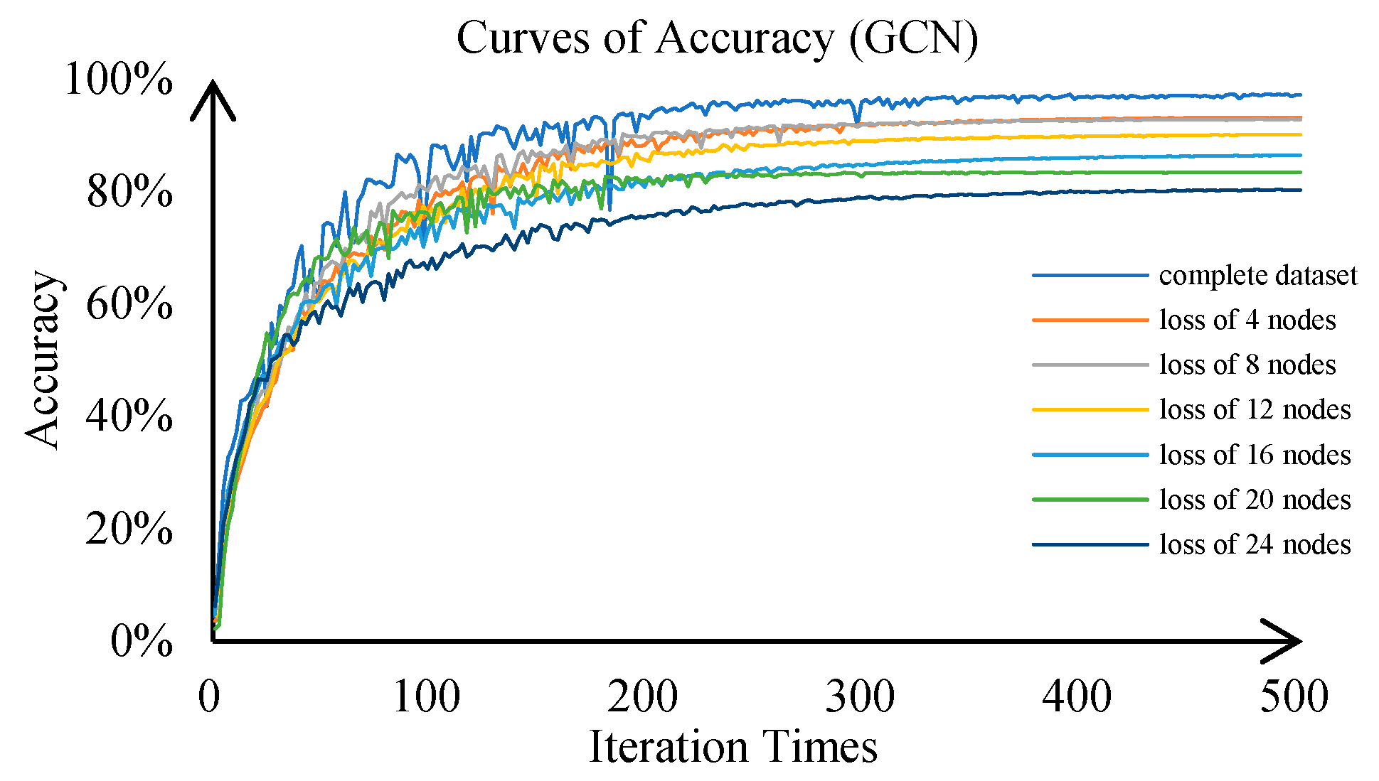
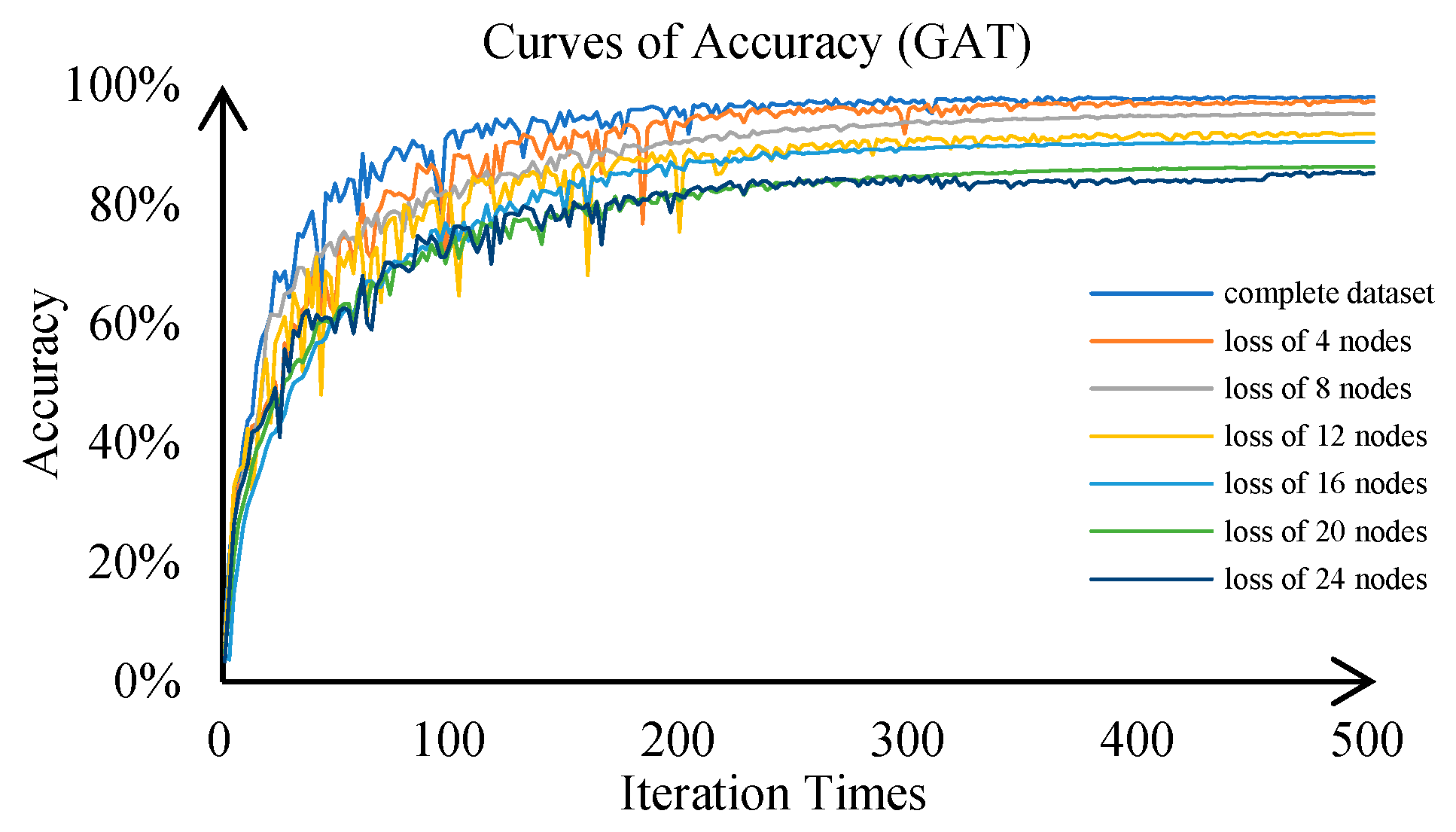
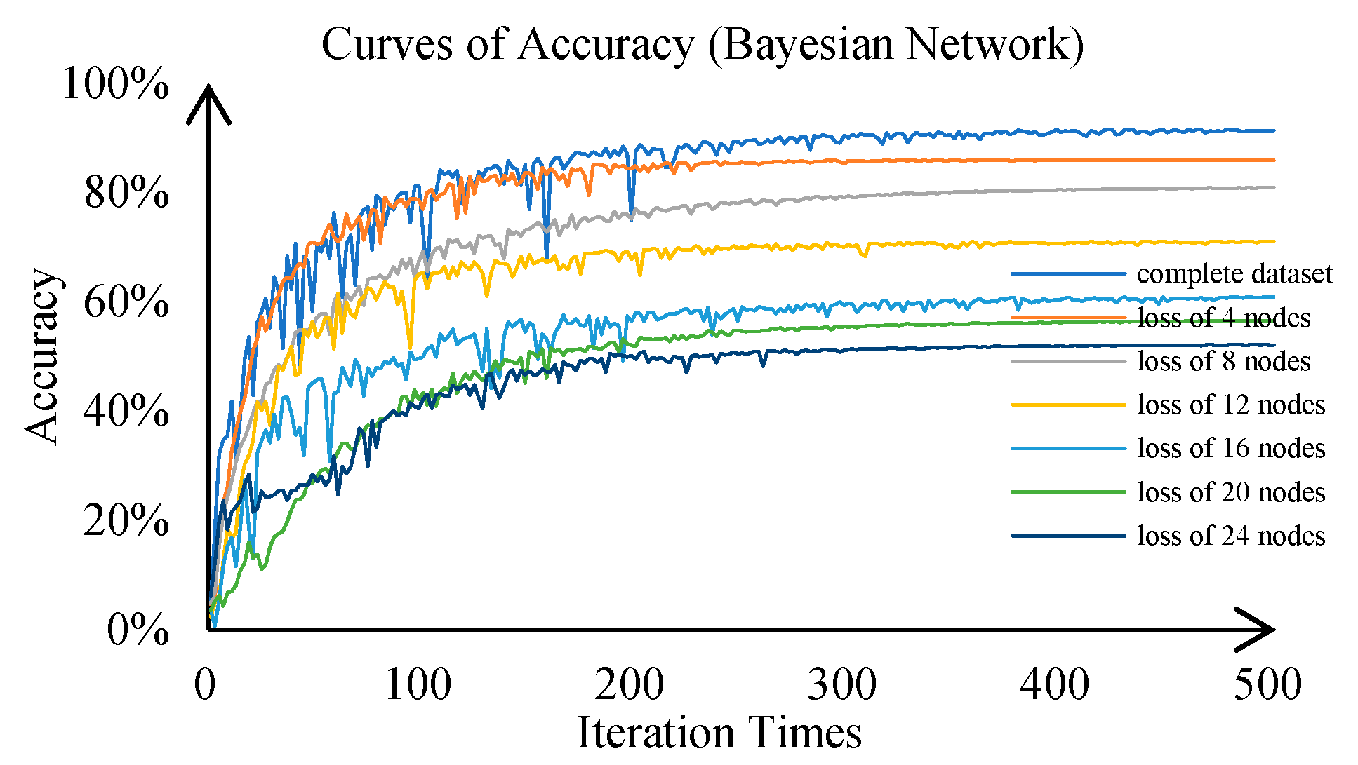
| Complete dataset | 98.59% | 97.15% | 98.08% | 95.38% | 91.32% |
| Loss of 4 nodes | 97.35% | 93.13% | 97.25% | 92.33% | 85.93% |
| Loss of 8 nodes | 95.32% | 92.81% | 95.24% | 89.42% | 80.89% |
| Loss of 12 nodes | 95.13% | 90.07% | 91.89% | 84.5% | 71.01% |
| Loss of 16 nodes | 94.67% | 86.42% | 90.57% | 79.18% | 60.83% |
| Loss of 20 nodes | 92.19% | 83.36% | 86.42% | 73.49% | 56.52% |
| Loss of 24 nodes | 89.79% | 80.24% | 85.35% | 66.31 | 52.13% |
| Connection relationship changes from bus26–bus28 to bus27–bus28 | 97.86% | 94.75% | 96.37% | 91.42% | 86.13% |
| Add connection relationship bus19–bus23 | 97.63% | 94.28% | 95.84% | 91.14% | 84.75% |
| Range | Number | Proportion |
|---|---|---|
| [0, 0.5%) | 185 | 6.72% |
| [0.5%, 1%) | 552 | 20.04% |
| [1%, 1.5%) | 639 | 23.20% |
| [1.5%, 2%) | 784 | 28.47% |
| [2%, 2.5%) | 335 | 12.16% |
| [2.5%, 3%) | 201 | 7.30% |
| [3%, 3.5%) | 45 | 1.63% |
| [3.5%, 4%) | 13 | 0.47% |
Disclaimer/Publisher’s Note: The statements, opinions and data contained in all publications are solely those of the individual author(s) and contributor(s) and not of MDPI and/or the editor(s). MDPI and/or the editor(s) disclaim responsibility for any injury to people or property resulting from any ideas, methods, instructions or products referred to in the content. |
© 2025 by the authors. Licensee MDPI, Basel, Switzerland. This article is an open access article distributed under the terms and conditions of the Creative Commons Attribution (CC BY) license (https://creativecommons.org/licenses/by/4.0/).
Share and Cite
Wang, F.; Hu, Z. A Novel Fault Diagnosis and Accurate Localization Method for a Power System Based on GraphSAGE Algorithm. Electronics 2025, 14, 1219. https://doi.org/10.3390/electronics14061219
Wang F, Hu Z. A Novel Fault Diagnosis and Accurate Localization Method for a Power System Based on GraphSAGE Algorithm. Electronics. 2025; 14(6):1219. https://doi.org/10.3390/electronics14061219
Chicago/Turabian StyleWang, Fang, and Zhijian Hu. 2025. "A Novel Fault Diagnosis and Accurate Localization Method for a Power System Based on GraphSAGE Algorithm" Electronics 14, no. 6: 1219. https://doi.org/10.3390/electronics14061219
APA StyleWang, F., & Hu, Z. (2025). A Novel Fault Diagnosis and Accurate Localization Method for a Power System Based on GraphSAGE Algorithm. Electronics, 14(6), 1219. https://doi.org/10.3390/electronics14061219