An Index of Refraction Adaptive Neural Refractive Radiance Field for Transparent Scenes

Abstract

Reconstructions and novel view syntheses of transparent object scenes are of great significance in numerous fields such as design, animation, and scientific research. The refraction of transparent objects brings challenges to the reconstruction of the geometry and radiance fields. Traditional photogrammetry methods and Neural Radiance Fields (NeRFs) establish geometric relationships based on the rectilinear propagation of light rays and thus fail in refraction scenes. In addition, different transparent objects have significantly different indexes of refraction (IORs) due to differences in materials, which pose challenges to the training of refraction radiance fields based on ray tracing. We propose a refractive radiance field method for the novel view synthesis of transparent object scenes. The method can reconstruct the geometry and radiance field using only a sequence of scene images of transparent objects, and it can automatically search for the optimal IOR without prior information. Our method consists of three stages, including geometric reconstruction, radiance field training, and IOR optimization. We verified our method on different datasets. In terms of its indicators, it is close to previous refraction radiance fields and other relatively advanced transparent scene rendering methods, while possessing higher flexibility.

1. Introduction

Transparent objects are extremely common in daily life, such as glass, plastics, or water. They play a non-negligible role in our daily lives. The rendering of scenes containing transparent objects is of great significance in fields like design, animation, and scientific research. To achieve the rendering of transparent object scenes, it is first necessary to conduct inverse rendering on the scenes. After obtaining the geometric, radiative, and other information of the scenes, the method of forward rendering can be adopted to synthesize images from novel views. However, the non-Lambertian characteristics of transparent objects make the inverse rendering of transparent objects difficult. The commonly used 3D reconstruction and radiance field reconstruction methods in computer vision are all designed based on the assumption of the rectilinear propagation of light. And the colors of transparent objects are completely determined by the transmitted or reflected ambient light, which leads to the failure of these common methods [1,2]. In addition, due to the strong refraction and reflection properties of transparent objects, general detection methods such as structured light [3,4] and photometric stereo vision [5] are also difficult to work well in such scenes.

Currently, many scholars have proposed different methods on inverse rendering and rendering transparent objects. Inverse rendering usually consists of two parts: 3D reconstruction in geometry and radiance field reconstruction in radiance. In the following sections, these methods will be introduced.

1.1. Three-Dimensional Reconstruction Methods for Transparent Objects

The reconstruction methods for general scenes are relatively mature, but the influence brought by refraction will make many existing methods ineffective for transparent objects [2]. Refraction causes the surface color of transparent objects to be related to the viewing angle, resulting in the failure of feature matching between views and thus the failure of reconstruction. One solution is to smear substances such as pigments on the surface of transparent objects. By avoiding refraction, the accuracy of feature matching can be ensured. It is also possible to immerse lens-shaped objects in liquid and then conduct reconstruction using Archimedes’ principle [6] or tomography [7,8]. However, such methods may cause damage to transparent objects, which limits their application range.

Non-contact methods can avoid causing damage, but they often require relatively complex equipment. Some methods directly adopt a scanning-like approach for reconstruction without relying on the refraction characteristics of transparent objects, such as specially designed line laser plane mirrors [9], RGB-D cameras [10], lasers [11], and scanners in the thermal infrared or ultraviolet bands [12,13,14]. There are also many methods that encode the scene and conduct the reconstruction of transparent objects according to the encoded values that are deformed after refraction and reflection [15,16]. Some scholars combine fringe screens for position encoding and combine multilayer perceptrons for the reconstruction of transparent objects [17]. Many methods conduct reconstruction based on the normal consistency of the same point on the object surface, such as the measurement method based on mobile display screens [18] or the improved triangulation reconstruction method [15]. They reconstruct multiple corresponding 3D coordinate points at each pixel to fit the possible refraction paths.

The environment matting technique solves the deformation of the background by transparent objects, enabling it to be composited onto different backgrounds [19,20]. However, the above methods have complex processes and all require specific equipment, such as specific display screens or turntables to assist the methods. Moreover, most methods require the known IOR, have a large number of assumptions and high computational complexity. Ihrke et al. [21] have conducted a detailed review on the 3D reconstruction of transparent objects.

1.2. Radiance Field Reconstruction Methods

According to the degree of restoration from low to high, the reconstruction of radiance fields is mainly divided into three types: view-independent radiance field reconstruction, view-dependent radiance field reconstruction, and illumination–material reconstruction. The first type of methods simply restores the radiance at each position of the scene at the time of taking pictures. The view-dependent radiance field reconstruction takes into account the change in radiance brought about by the change in viewing angle and obtains novel views using the rendering equation. The illumination–material reconstruction decouples the radiance field and reconstructs the illumination and the material of the object separately. This method enables the manipulation of illumination and material properties and has more flexible application scenarios.

In recent years, methods based on differentiable rendering have developed relatively rapidly [22,23]. Currently, the most commonly used method is the Neural Radiance Field (NeRF) [24] series. This method models the entire scene as a radiance field. The color and volume density at a certain position in the radiance field depend on the position and the viewing angle to achieve anisotropic rendering effects, and then the rendering image is obtained using forward rendering according to the radiation transfer equation. The parameters of the neural network are updated according to the gradient calculated from the difference between the rendered image and the real image. On the one hand, such methods can learn only with visible light images and camera poses. Many scholars have optimized the rendering accuracy and speed of NeRF from multiple aspects, such as position encoding, up to now [25,26,27,28].

Some scholars have modified the luminous particles in NeRF into luminous and reflective particles and reconstructed the direct illumination, indirect illumination, and material at each position when the position of the light source is known [29], but this method is not applicable to general scenes. There are methods to calculate the normal by taking the gradient of the volume density [30]. Jin et al. [31] directly uses neural networks to calculate the normal. Li et al. [32] reconstructs the normal through dense point clouds. Regarding the propagation process of light rays, those methods use neural network visibility estimation networks to model direct light and scattered light. Generally speaking, due to the implicit representation of NeRF, the estimation of the normal is not accurate and the phenomenon of being overly smooth may occur.

To accurately express the geometric shape of the object surface, Wang et al. [33] used the Signed Distance Function (SDF) to store the scene, adopted the Neural Signed Distance Field (NeuS) to fit the SDF at each position, and derived the corresponding relationship between the SDF value at a certain position in space and the volume density in NeRF according to the rendering equation, so as to use the same radiation transfer equation as NeRF for rendering. There are many studies on inverse rendering based on NeuS [34,35,36]. Most of these methods are similar to the inverse rendering process based on NeRF, that is, using neural networks to estimate the SDF, material, indirect illumination, and direct illumination. The only difference is that the SDF can provide more accurate normals and more direct occlusion information, which is convenient for obtaining more accurate normals and direct light.

The point-based scene representation method can effectively render unstructured point cloud samples [37,38] and can use parallel computing to complete rasterization imaging [37,39]. Kerbl et al. [40] set the points as Gaussian ellipsoids and established a fast rasterization process based on this for rendering and gradient backpropagation. This method uses the gradient for adaptive ellipsoid density control, enabling the ellipsoids to be completely and accurately covered on the object surface guided by the gradient. While having a rendering effect comparable to that of NeRF, its speed far exceeds that of NeRF. Since the method can be calculated in parallel and does not require inference, it can achieve a rendering speed of more than 100 frames per second.

Although the above methods can provide rendering effects with a sense of realism, they do not restore illumination and materials and cannot perform relighting. Some scholars have restored the materials of each Gaussian sphere using ray tracing between Gaussian spheres [41]. During the training process of 3D Gaussian spheres, they will tend to be flattened to fit the surface of objects. Inspired by this phenomenon, some scholars initialize the shortest axis of the ellipsoid as the normal of the ellipsoid and add small residuals to correct the surface [42,43]. The former still adopts a relatively complete Bidirectional Reflectance Distribution Function (BRDF) modeling scheme and determines visibility using single-stage ray tracing to decompose direct light and indirect light, while the latter sets a unified diffuse color for the range covered by each Gaussian sphere and only calculates the specular reflection color to improve computational efficiency. It improves the sense of realism while retaining the real-time rendering ability of 3D Gaussian splatting. However, due to the inconsistency between the distribution of 3D ellipsoids and the actual surface distribution, the assumption of regarding the short axis of the ellipsoid as the normal still has relatively large errors.

1.3. Radiance Field Reconstruction Methods for Transparent Object Scene

In the method described in Section 1.2, light still travels in a straight line. Although some algorithms have considered the reflection effect, these algorithms are not designed for the refraction characteristics of transparent objects. These methods will cause serious blurring and artifacts during the reconstruction process of transparent objects. For the reconstruction of the radiance field in transparent object scenes, Bemana et al. [44] introduced the eikonal equation to optimize the IOR field on the light propagation path, and Pan et al. [45] further proposed the hierarchical path sampling technique to improve surface details and clarity. Sun et al. [46] proposed a two-stage method for the three-dimensional reconstruction of nested transparent objects. In the first stage, the environmental radiance field and the outer surface are reconstructed, and the Multi-Layer Perceptron (MLP) is used to approximate the refracted light. In the second stage, ray tracing is used to reconstruct the internal surface. However, this method requires manually specifying the transparent parts in the three-dimensional scene and requires prior information on the IOR.

The Neural Refractive Radiance Field (NeRRF) [47] decomposes the rendering problem into two parts: geometric reconstruction and ray tracing rendering. First, the object is reconstructed in three dimensions by using the Deep Marching Tetrahedra (DMTet) [48] algorithm combined with masks. Then, ray tracing is carried out according to the IOR, and sampling and radiance field training are performed on the modified light path. However, this method requires ray tracing for each outgoing light ray, and the training and novel view synthesis speeds are extremely slow. Moreover, in actual situations, it is difficult to obtain the accurate IOR of transparent objects, which brings difficulties to accurate ray tracing and limits the use of this method.

We make improvements based on NeRRF and propose an IOR-adaptive inverse rendering method, which can perform surface reconstruction and radiance field reconstruction of transparent objects only based on a sequence of scene images of transparent objects, and then conduct novel view synthesis according to the reconstructed scene. The main contributions of this paper are as follows:

• A framework for scene reconstruction and novel view synthesis that only relies on a set of multi-view transparent object scene images or videos without any other prior knowledge.
• An IOR estimation algorithm that can automatically search for the best IOR during the process of radiance field training, which ensures the accuracy of subsequent radiance field training without the need for an accurate IOR value.
• We correct the inaccurate calculation method of the refractive effect in NeRRF, enabling us to render the phenomenon of the foreground darkening caused by refraction more accurately, especially at the edges.
• A mask-based ray-tracing acceleration algorithm that can reduce the training time by approximately 60% and rendering time by 75%.
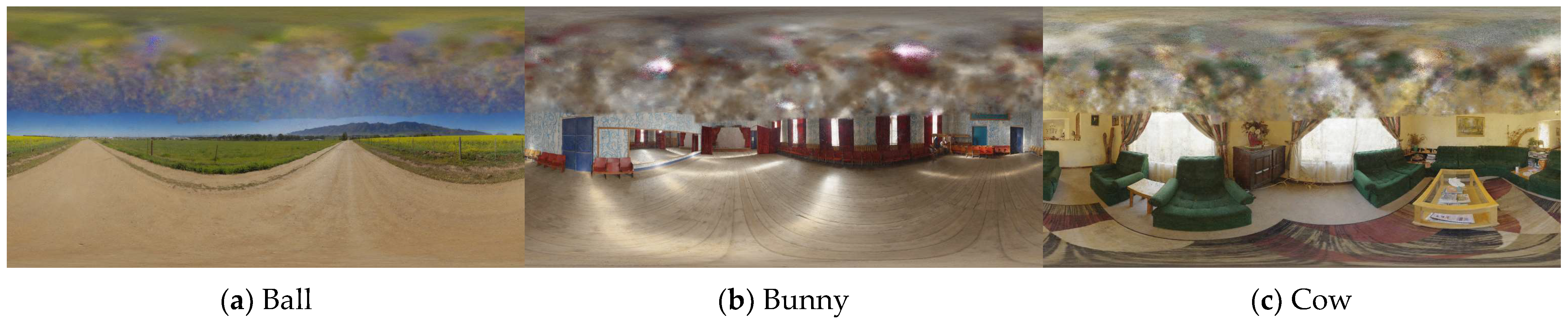
• Our method performs complete inverse rendering on the scene to obtain relatively accurate ambient light, transparent object geometry, and IOR, enabling various downstream tasks such as object editing, environment editing, and IOR editing.

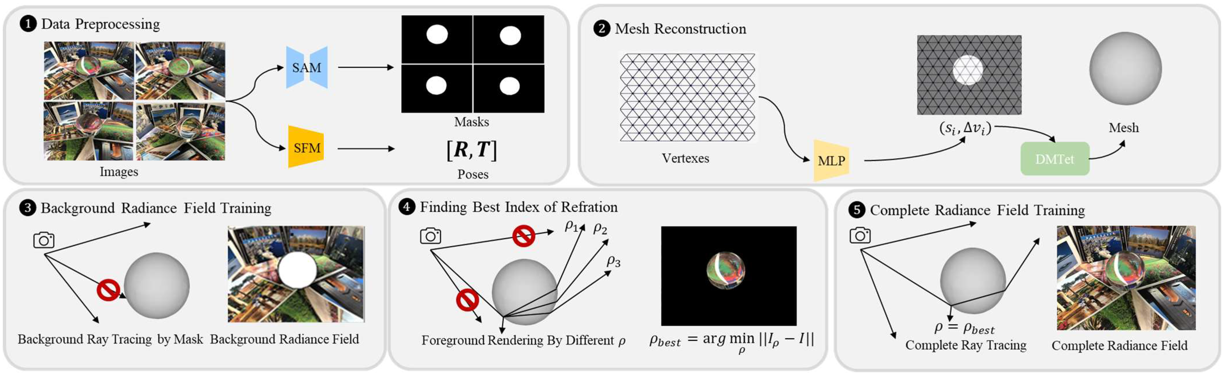
2. IOR-Adaptive Refraction Scene Reconstruction Method

In this section, an IOR adaptive refraction scene reconstruction method, including a 3D reconstruction and novel view synthesis framework, is proposed. This framework includes the DMTet 3D reconstruction algorithm and the refractive radiance field algorithm. In addition, the ray-tracing acceleration module with masks and the IOR optimization module are incorporated.

This method follows a series of steps, including data preprocessing, mesh reconstruction based on DMTet, background radiance field training, best IOR searching, and complete radiance field training. The method architecture is shown in Figure 1.

Data preprocessing mainly includes mask extraction based on the Segment Anything Model (SAM) [49] and camera pose reconstruction based on Structure from Motion (SfM) [50]. Next, the camera poses and masks were used to reconstruct the surface geometry using DMTet. Then, the radiance field was trained. Firstly, the background radiance field was trained in combination with the masks. Subsequently, the foreground was rendered according to the trained background radiance field using different IORs, and the IOR that maximized the Peak Signal-to-Noise Ratio (PSNR) of the foreground was selected as the optimal IOR. Finally, training the complete radiance field was carried out.

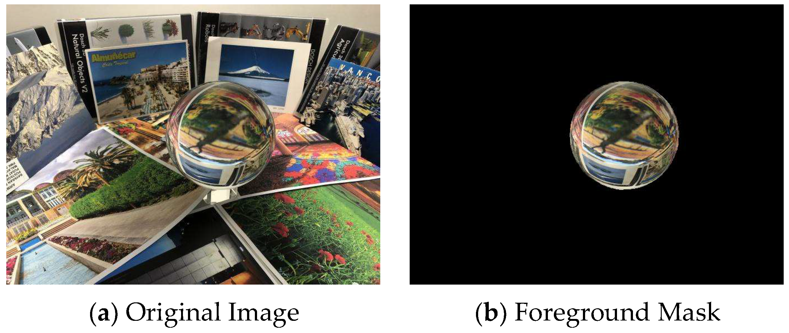
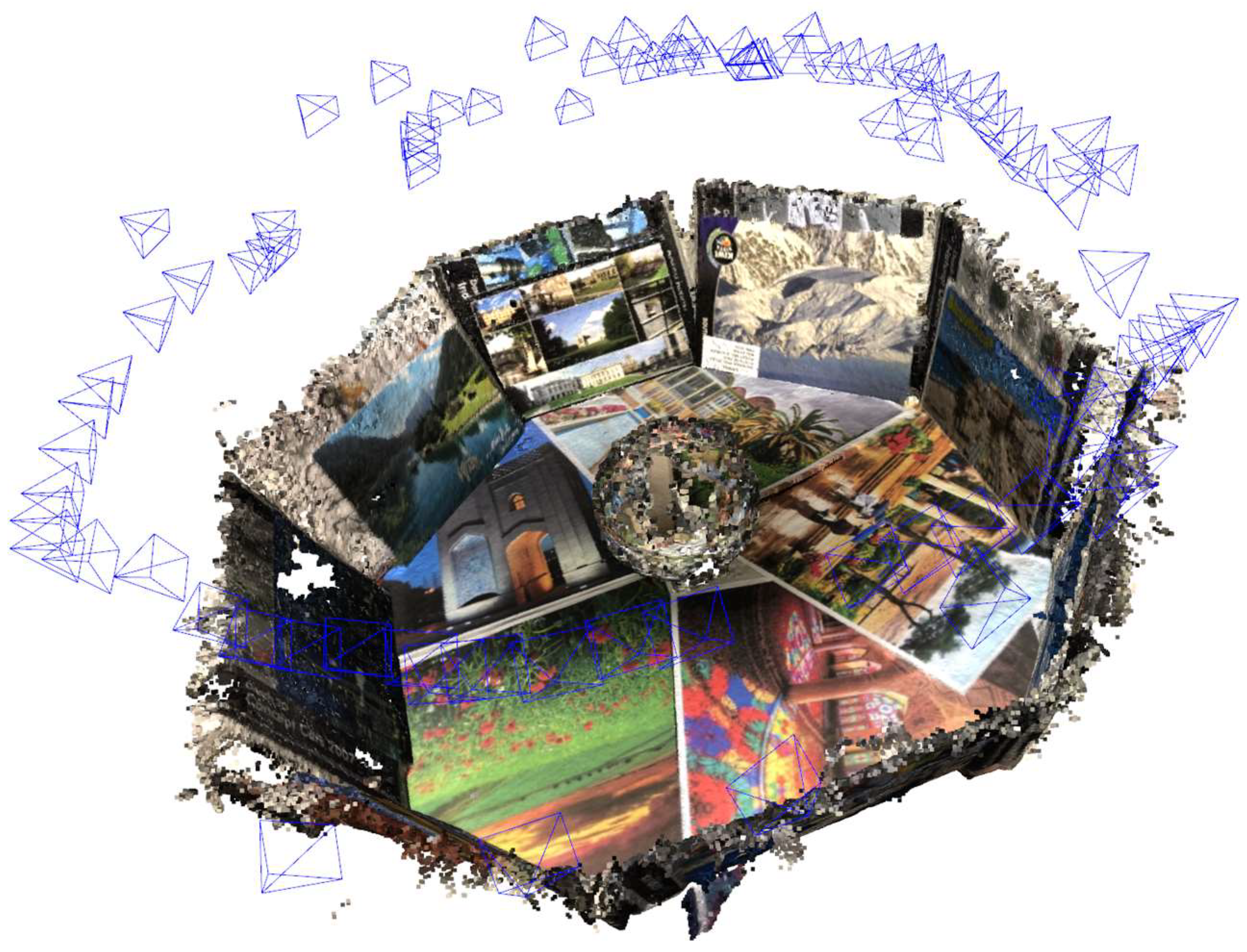
2.1. Data Preprocessing

The training of DMTet and NeRF requires the masks of objects and the camera poses of images as supervision. We extracted masks based on the SAM. The pre-trained SAM was used to obtain all of the masks of the pictures first. Then, the $top-3$ matching masks for the remaining pictures were automatically selected and stored based on their position information, color histograms, and mask sizes. The intersection of the above three masks is taken, and the largest connected region in terms of area is extracted as the best mask. Subsequently, we eliminate the burrs in the masks using the opening operation. We repaired excessively inaccurate masks manually, but, in fact, most masks were of reliable quality. In addition, the deviation in a few pixels at the boundary did not have an excessive impact on the subsequent geometric reconstruction effect, as shown in Section 3.2.1. The recovery of camera poses was completed using the open-source software COLMAP 3.8 [50].

2.2. Mesh Reconstruction

After obtaining the masks and camera poses, we used DMTet to conduct surface reconstruction for the object. This algorithm defines the geometric shape of the object as a SDF on the mesh $T$. Each vertex $v_i$ on $T$ is characterized by an SDF value $S_i\in R$ and a deformation value ${∆v}_i\in R^3$. In each update, the mesh is deformed as ${v_i^{\prime }=v_i+∆v}_i$. In order to obtain an explicit mesh, the DMTet is used to extract the surface of the object from the mesh.

This process is supervised by the object masks. The object is projected according to the camera pose to obtain the rendered masks. We use $L_1$ loss for training.

$$L_{mask}={\left|\left|M-M^{\prime }\right|\right|}_2$$

(1)

Directly optimizing the SDF values of each vertex in the mesh may introduce high-frequency noise. Adopting position encoding with a lower frequency can effectively alleviate this problem, but it will lead to the loss of important high-frequency details during the reconstruction process. Therefore, this paper employs progressive position encoding [47]. The encoding frequency is gradually increased after the training has reached a certain stage so as to minimize noise while retaining details.

During the reconstruction process using DMTet, implicit geometric regularization (IGR) [51] is added. The regularization term is added to the training in the form of eikonal loss to constrain the gradient magnitude of the SDF field to be close to 1 [51]:

$$L_{eikonal}=E_{v_0\in V_0}{\left(||\nabla f_{\theta }\left(v_0\right){\left|\right|}_2-1\right)}^2$$

(2)

2.3. Radiance Field Training and IOR Optimization Based on Ray Tracing

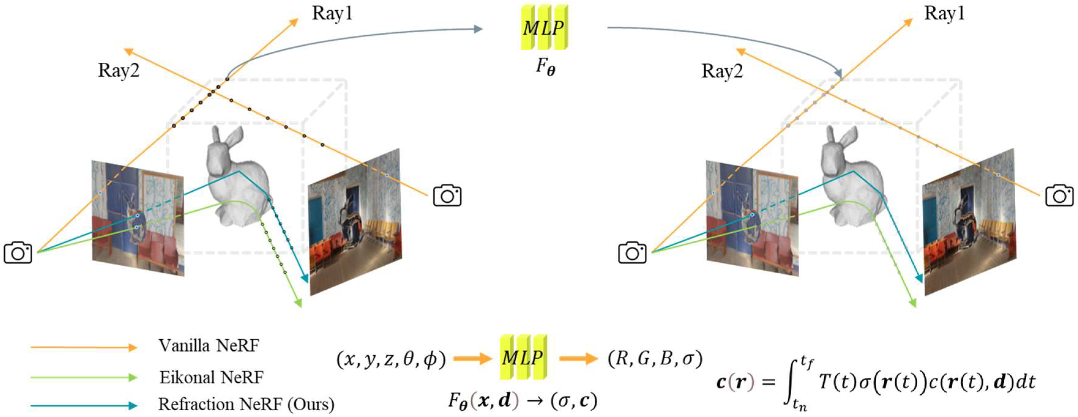
2.3.1. Neural Radiance Field

We used NeRF, a new and efficient way of representing the radiance field, to reconstruct the radiance field. The process of NeRF is shown by the orange arrows in Figure 2. NeRF represents the radiance field of a scene as a five-dimensional function $F_{\mathit{\theta }}\left(\mathit{x},\mathit{d}\right)\to (\sigma ,\mathit{c})$, where $\mathit{x}=(x,y,z)$ represents the 3D position, $\mathit{d}=\left(\theta ,\varphi \right)$ represents the view direction, $\sigma$ represents volume density, and $\mathit{c}=[R,G,B]$ represents the radiance in the R, G, and B bands. NeRF uses a single MLP to represent the neural radiance field and performs rendering according to the rendering equation. For a ray $\mathit{r}=\mathit{o}+t\mathit{d}$ emitted by a camera located at point $\mathit{o}$, the color value of the corresponding pixel is as follows:

$$\mathit{c}\left(\mathit{r}\right)={\int }_{t_n}^{t_f}T\left(t\right)\sigma \left(\mathit{r}\right(t\left)\right)\mathit{c}(\mathit{r}\left(t\right),\mathit{d})dt$$

(3)

where $T\left(t\right)=\mathrm{e}\mathrm{x}\mathrm{p}(-{\int }_{t_n}^t\sigma \left(\mathit{r}\right(s\left)\right)ds)$.

In order to calculate the integral using the program, the rendering equation is discretized by a stratified sampling approach:

$$t_i\sim U[t_n+{\displaystyle \frac{i-1}{N}}\left(t_f-t_n\right),t_n+{\displaystyle \frac{i}{N}}(t_f-t_n)]$$

(4)

The propagation path of the light ray is divided into $N$ parts and randomly samples a point in each interval according to a uniform distribution to calculate the integral:

$$\widehat{\mathit{c}}\left(\mathit{r}\right)=\sum _{i=1}^N{T}_i\left(1-\exp \left(-{\sigma }_i{\delta }_i\right)\right){\mathit{c}}_i$$

(5)

where $T_i=\mathrm{e}\mathrm{x}\mathrm{p}(-\sum _{j=1}^{i-1}{\sigma }_j{\delta }_j)$.

To enable the network to learn higher-frequency information, position encoding is used to map the original input to a high-dimensional space. In the original NeRF, the trigonometric function encoding method was adopted. Müller et al. [52] proposed Instant-NGP, a position encoding method with multi-resolution hash encoding. It improves the representational ability of the scene while reducing the number of network parameters and increasing the rendering speed. In this paper, we use this method to perform position encoding.

During the initial training, since the positions of the objects are unknown and the weights of each position for the color during the light propagation process cannot be determined, a uniform sampling method is adopted, which is called coarse sampling. After the coarse sampling is completed, the positions where the objects exist in the scene are roughly determined. On this basis, NeRF conducts fine sampling based on the volume density of each position on the light path as the weight to improve the detail representation. The final loss includes the color loss of the coarse sampling and fine sampling:

$$L=\sum _{r\in R}[{‖{\widehat{\mathit{c}}}_{\mathit{c}}\left(\mathit{r}\right)-\mathit{c}\left(r\right)‖}_2+{‖{\widehat{\mathit{c}}}_{\mathit{f}}\left(\mathit{r}\right)-\mathit{c}\left(r\right)‖}_2]$$

(6)

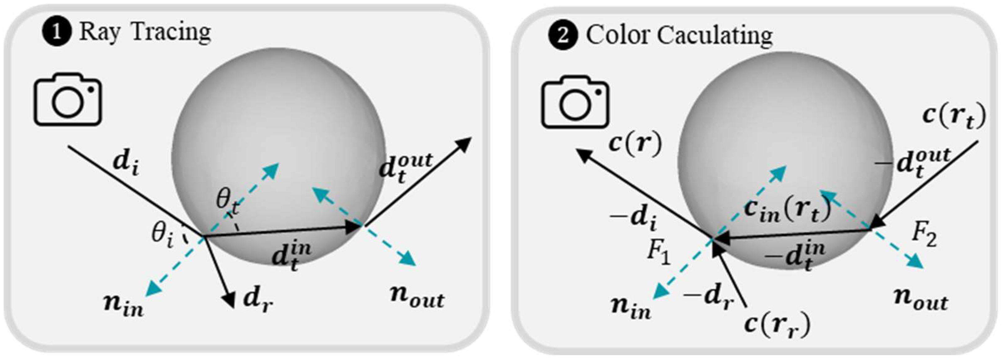
2.3.2. Refraction Radiance Field

We performed pixel-by-pixel ray tracing on the images to modify the light path based on the surface reconstructed. The process is shown by the blue arrows in Figure 2. Firstly, we calculate the intersection of each ray with the transparent object. For rays that do not intersect with the object, there is no need to modify the light path, and color rendering can be directly calculated according to Equation (5). Additionally, when conducting radiance field training using the simulation dataset based on Blender, the ambient light can be regarded as being at an infinite distance, and the color is only related to the viewing direction. At this time, the color and volume density of each sampling point in space are represented as $F_{\sigma ,\mathit{c}}\left(\mathit{d}\right)\to (\sigma ,\mathit{c})$.

For rays that intersect with the transparent object, since the object itself is colorless, the color of the transparent object depends only on the color of the emergent rays. It is necessary to calculate the outgoing direction of light rays through ray tracing to obtain the correct color of the incident points. The process of ray tracing is shown in Figure 3.

The rays will refract according to Snell’s law. The IOR of air is approximately 1. For a ray $\mathit{r}=\mathit{o}+t{\mathit{d}}_{\mathit{i}}$ that intersects with the object, and where the IOR of the object is $\eta$, the cosine value of the refraction angle $cos{\theta }_t$ is as follows:

$$cos{\theta }_t=\sqrt{1-{\sin }^2{\theta }_t}=\sqrt{1-{\eta }^2(1-{\cos }^2{\theta }_i)}$$

(7)

and refracted ray direction ${\mathit{d}}_{\mathit{r}}=2\mathit{n}\left({\mathit{d}}_{\mathit{i}}\cdot \mathit{n}\right)-{\mathit{d}}_{\mathit{i}}$, reflected ray direction ${\mathit{d}}_{\mathit{t}}=-\eta {\mathit{d}}_{\mathit{i}}+(\eta \left({\mathit{d}}_{\mathit{i}}\cdot \mathit{n}\right)-\mathrm{c}\mathrm{o}\mathrm{s}({\theta }_t)\mathit{n}$.

Suppose that the ray intersects the object at point $\mathit{p}$, then the reflected ray is ${\mathit{r}}_{\mathit{r}}=\mathit{p}+t{\mathit{d}}_{\mathit{r}}$ and the refracted ray is ${\mathit{r}}_{\mathit{t}}=\mathit{p}+t{\mathit{d}}_{\mathit{t}}$. When the radiance of the ray is $L$, the ratio of the radiance of the reflected ray $L_r$ and that of the refracted ray $L_t$ is given by Fresnel’s law:

$$F={\displaystyle \frac{1}{2}}{\left({\displaystyle \frac{{\mathit{d}}_{\mathit{i}}\cdot \mathit{n}-\lambda {\mathit{d}}_{\mathit{t}}\cdot \mathit{n}}{{\mathit{d}}_{\mathit{i}}\cdot \mathit{n}+\lambda {\mathit{d}}_{\mathit{t}}\cdot \mathit{n}}}\right)}^2+{\displaystyle \frac{1}{2}}{\left({\displaystyle \frac{{\lambda \mathit{d}}_{\mathit{i}}\cdot \mathit{n}-{\mathit{d}}_{\mathit{t}}\cdot \mathit{n}}{{\lambda \mathit{d}}_{\mathit{i}}\cdot \mathit{n}+{\mathit{d}}_{\mathit{t}}\cdot \mathit{n}}}\right)}^2,$$

(8)

$$L_r=FL, L_t=\left(1-F\right)L.$$

(9)

We only perform ray tracing twice for each light to obtain the initial incident light and the emergent light. For the case shown in Figure 3, the color c received by the camera is weighted by the color ${\mathit{c}}_{\mathit{r}}$ reflected by the object and the refracted light ct emitted from the object according to Fresnel’s law. We can calculate the Fresnel coefficient of the incident light $F_1$ and the Fresnel coefficient of the emergent light $F_2$ after ray tracing using Equation (8). Then, the color inside the object ${\mathit{c}}_{\mathit{i}\mathit{n}}\left({\mathit{r}}_{\mathit{t}}\right)$ is

$${\mathit{c}}_{\mathit{i}\mathit{n}}\left({\mathit{r}}_{\mathit{t}}\right)=\left(1-{\mathit{F}}_2\right)\mathit{c}\left({\mathit{r}}_{\mathit{t}}\right).,$$

(10)

Finally, the color of the pixel is determined simultaneously by the color $\mathit{c}\left({\mathit{r}}_{\mathit{r}}\right)$ of the light reflected into the camera and the color ${\mathit{c}}_{\mathit{i}\mathit{n}}\left({\mathit{r}}_{\mathit{t}}\right)$ of the light refracted into the camera:

$$\mathit{c}\left(\mathit{r}\right)=F_1\mathit{c}\left({\mathit{r}}_{\mathit{r}}\right)+\left(1-F_1\right){\mathit{c}}_{\mathit{i}\mathit{n}}\left({\mathit{r}}_{\mathit{t}}\right),$$

(11)

$$\mathit{c}\left(\mathit{r}\right)=F_1\mathit{c}\left({\mathit{r}}_{\mathit{r}}\right)+\left(1-F_1\right)(1-F_2)\mathit{c}\left({\mathit{r}}_{\mathit{t}}\right).$$

(12)

The loss function for training adopts Equation (6) and optimizes the color values of both coarse sampling and fine sampling simultaneously.

It should be noted that NeRRF complies simply with the law of conservation of energy. They simply set the weight sum of reflected light and refracted light to 1, which does not conform to the real situation. The ray tracing process only simulates the interaction between the outgoing light of the camera and the object. It can provide us with accurate Fresnel coefficients $F$ and the direction of refracted and reflected rays. When calculating the final color, forward rendering based on the above results is more consistent with physical principles. Since there is no $(1-F_2)$ term in the color calculation method, the color of the foreground tends to be brighter, especially at the edges. Although this way of calculating colors slightly violates the law of conservation of energy, it best conforms to the propagation rules of direct light. The missing terms mainly come from reflections and scatterings in other directions inside the object.

During the ray tracing process, finding the intersection of each ray with the object is a very time-consuming process. In this paper, mask information is added during the ray tracing process. Since only the rays emitted by the foreground pixels will intersect with the object, other pixels will definitely not intersect with the object. Therefore, during the training and rendering processes, only the pixels with a mask value of $1$ are traced. To ensure that our mask can completely cover all intersecting pixels, we added a buffer of 5 pixels on the basis of the mask obtained using SAM. This operation will bring some redundant calculation of non-foreground pixels, but can achieve an accurate ray tracing effect. Note that only the mask used for this step will be added to the buffer, and the mask used for geometric reconstruction will not. This operation can reduce the training time by approximately 60% and the rendering time by 70–80% depending on the proportion of the foreground.

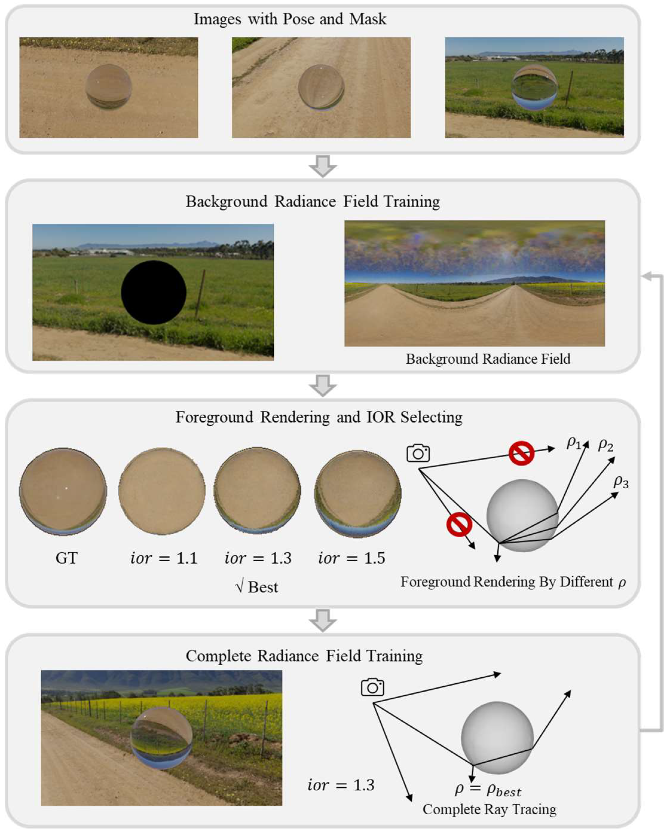
2.3.3. IOR Optimization

In practical applications, obtaining the accurate IOR is difficult. Influenced by the work of Pan et al. [45] and Sun et al. [46], we propose an algorithm for adaptively optimizing the IOR, which iteratively obtains the optimal IOR during the training process. The algorithm is shown in Figure 4.

This algorithm mainly includes three steps: (1) background radiance field training, (2) foreground rendering and IOR selecting, and (3) complete radiance field training. Firstly, the colors of the pixels with a mask value of 0, representing the background radiance field, are trained. Studies have proved that the background radiance field is basically not affected by refraction [45,46] and can provide a reference for the IOR. After several rounds of training, we obtain a basically correct background radiance field. Since the color of the transparent object depends only on the ambient light, we believe that only with the background radiance field and the correct IOR can we obtain the correct rendering effect.

Subsequently, we searched for the best IOR within a possible IOR interval. The interval was evenly divided into ten equal parts, and each partition value was used to render the foreground, respectively. The IOR that minimizes the Mean Squared Error (MSE) between the foreground rendered image and the real image was found:

$$IO{R}_{best}=\underset{\mathit{IOR}}{\max }PSNR({\mathit{c}}_{\mathit{i}\mathit{o}\mathit{r}}\left(\mathit{r}\right),{\mathit{c}}_{\mathit{l}\mathit{a}\mathit{b}\mathit{e}\mathit{l}}\left(\mathit{r}\right)).$$

(13)

Then, with the intervals on both sides of this IOR as the new search interval, the optimal IOR was determined again to obtain the final optimal IOR. Finally, the rays of both the foreground and the background were trained simultaneously to train the few rays that only appeared in the foreground. The pseudo-code of the algorithm is shown in Algorithm 1.

Algorithm 1 Optimal IOR searching.

Input: A MLP $F_{\mathit{\theta }}\left(\mathit{x},\mathit{d}\right)\to (\sigma ,\mathit{c})$, IOR range $[IO{R}_{min}, IO{R}_{max}]$, the number of IOR search segments $k$, transparent object mesh $M$, foreground camera rays $\mathit{r}=\{{\mathit{r}}_{\mathbf{1}},\dots ,{\mathit{r}}_{\mathit{n}}\}$, foreground pixel color ${\mathit{c}}_{\mathit{l}\mathit{a}\mathit{b}\mathit{e}\mathit{l}}=\{{\mathit{c}}_{\mathbf{1}},\dots ,{\mathit{c}}_{\mathit{n}}\}$.

Output: Optimal IOR $IO{R}_{best}$.

1: Divide the IOR range into $k$ equal parts $IO{R}_{list}=[IO{R}_{min},\dots , IO{R}_{max}]$.

2: Init $PSN{R}_{max}=-\infty$, $IO{R}_{best}=IO{R}_{min}$

3: for ($i=1; i\le k; i++$) do 4:  $IO{R}_{now}=IO{R}_{list}\left[i\right]$ 5:  Calculate the emergent light rays after refraction ${\mathit{r}}_{\mathit{r}\mathit{e}\mathit{f}\mathit{r}}=RayTracing\left(\mathit{r}\right)$. 6:  Render color of each pixel by Equation (5), ${\mathit{c}}_{\mathit{I}\mathit{O}\mathit{R}}=\{{\mathit{c}}_{\mathbf{1}}^{\mathit{I}\mathit{O}\mathit{R}},\dots ,{\mathit{c}}_{\mathit{n}}^{\mathit{I}\mathit{O}\mathit{R}}\}$. 7:  Calculate $PSN{R}_{IOR}=\mathsf{\Sigma }{\left|\left|{\mathit{c}}_{\mathit{l}\mathit{a}\mathit{b}\mathit{e}\mathit{l}}-{\mathit{c}}_{\mathit{I}\mathit{O}\mathit{R}}\right|\right|}_2$ 8:  if $PSN{R}_{IOR}>PSN{R}_{max}$ then 9:   $IO{R}_{best}=IO{R}_{now}$ 10:   end if 11: end for 12: new IOR range $IO{R}_{range}^{new}=\left(IO{R}_{max}-IO{R}_{min}\right)\ast 0.4$ 13: Set the IOR range for the next search. $[IO{R}_{best}-IO{R}_{range}^{new}/2, IO{R}_{best}+IO{R}_{range}^{new}/2]$

14: return $IO{R}_{best}$

3. Experiments and Results

3.1. Experiment Settings

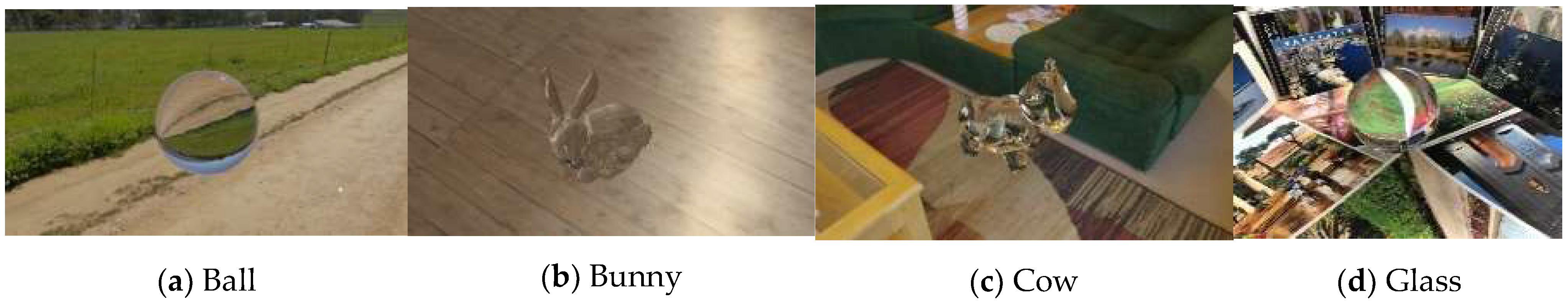
3.1.1. Dataset

We employed synthetic datasets based on Blender synthetic and real-scene datasets to test our method. Blender can accurately render the physical processes of light rays in scenes with transparent objects, including reflection and refraction. The synthetic dataset includes images, refractive indices, camera poses, and masks for training and evaluating the performance of different methods. This dataset consists of three groups, namely “Ball”, “Bunny”, and “Cow”, as shown in Figure 5a–c. The real dataset is the “Glass” dataset from [44], as shown in Figure 5d. We adopt the method in Section 2.1 to extract masks and poses. Figure 6 presents examples of images and extracted masks, and the poses reconstructed are illustrated in Figure 7.

3.1.2. Evaluation

We conducted comprehensive experiments on four groups of datasets to evaluate the performance of our method. These mainly included evaluations of the geometric reconstruction effect and evaluations of the novel view rendering effect. In addition, we also carried out some additional experiments, including ambient light reconstruction and scene and IOR editing.

For the reconstruction results, due to the lack of ground truth data, a qualitative comparison was made between the geometric structures reconstructed by the algorithm in this paper and those reconstructed by the commercial software Metashape 2.1.0 [53], which is specialized for 3D reconstruction. We also compared our method with NeuS [33], a relatively advanced 3D reconstruction algorithm based on deep learning.

For the rendering effect, PSNR, Structural Similarity Index Measure (SSIM), and Learned Perceptual Image Patch Similarity (LPIPS) were used to compare the rendered images in the test set with the real images. Meanwhile, the native NeRF algorithm encoded with Instant-NGP [52] was used as a benchmark for comparison. In addition, the approximately optimal IOR after IOR optimization was also compared with the true IOR to evaluate the IOR optimization algorithm.

3.1.3. Experimental Details

The algorithm in this paper is implemented based on PyTorch 1.10.0, and all experiments are conducted on a single NVIDIA A40.

1.

Details of Surface Reconstruction

The parameter settings for surface reconstruction adopted in this paper follow similar settings in NeRRF [47]. The position encoding adopts six-channel Fourier frequency encoding and is gradually activated during training. The learning rate for training is set to 0.01. Each scene undergoes three epochs of iteration. Each epoch traverses the dataset 50 times, and each traversal randomly samples a batch size of 640 pixels in the images for training. For the rabbit and cow, which have more high-frequency details, the coefficient of the eikonal loss is set to 0.01 in the first two epochs and 0.001 in the last epoch. For the sphere with fewer high-frequency details, this coefficient is set to 0.1 in the first two epochs and 0.001 in the last epoch.

2.

Details of Radiance Field Reconstruction

During training, we use Equation (6) as the loss function, and the coefficients of the coarse sampling loss term and fine sampling loss term are both set to 1. We use the Adam optimizer with a learning rate of 0.01. For the Blender dataset, each scene undergoes four epochs of iteration. Each epoch traverses the dataset 50 times, and each traversal randomly samples a batch size of 640 pixels in the images for training. For the real dataset, each scene undergoes eight epochs of iteration, and each epoch traverses the dataset 100 times. During the IOR optimization process, since the IOR of most transparent objects is within 1–2.5, the initial IOR search interval is set to [1, 2.5] and the number of search intervals is 10. We conducted an IOR search for every epoch during the training of the background radiance field, and then the foreground radiance field is trained for another epoch.

3.2. Experiment Results

In this section, we show the effect of this method on geometric reconstruction and new view synthesis tasks, respectively. At the same time, we also conducted ablation experiments and some supplementary experiments, mainly including ambient light reconstruction and scene editing.

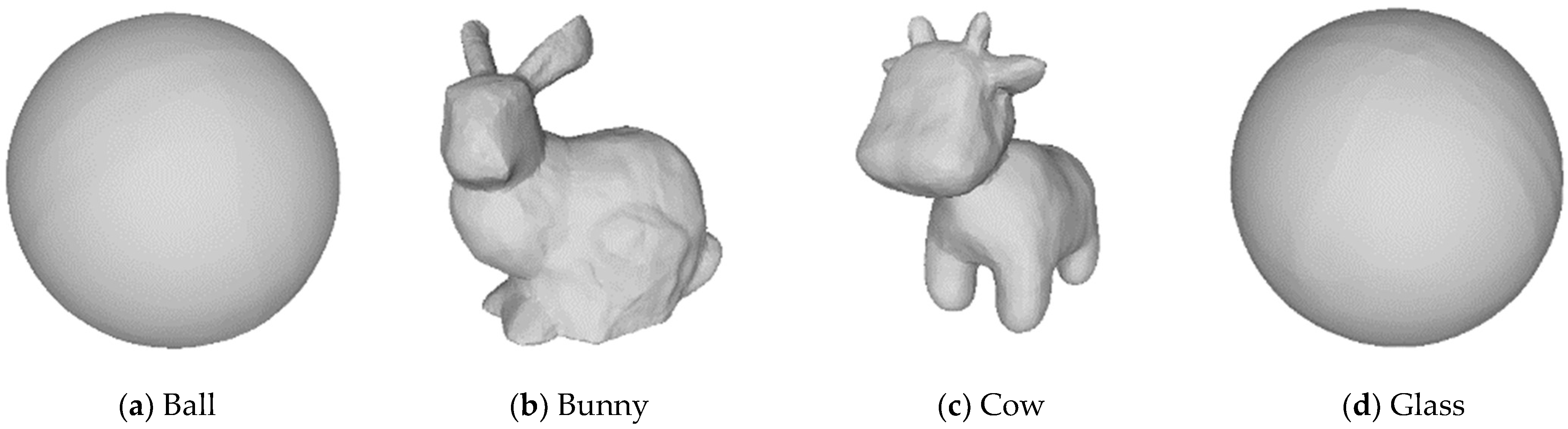
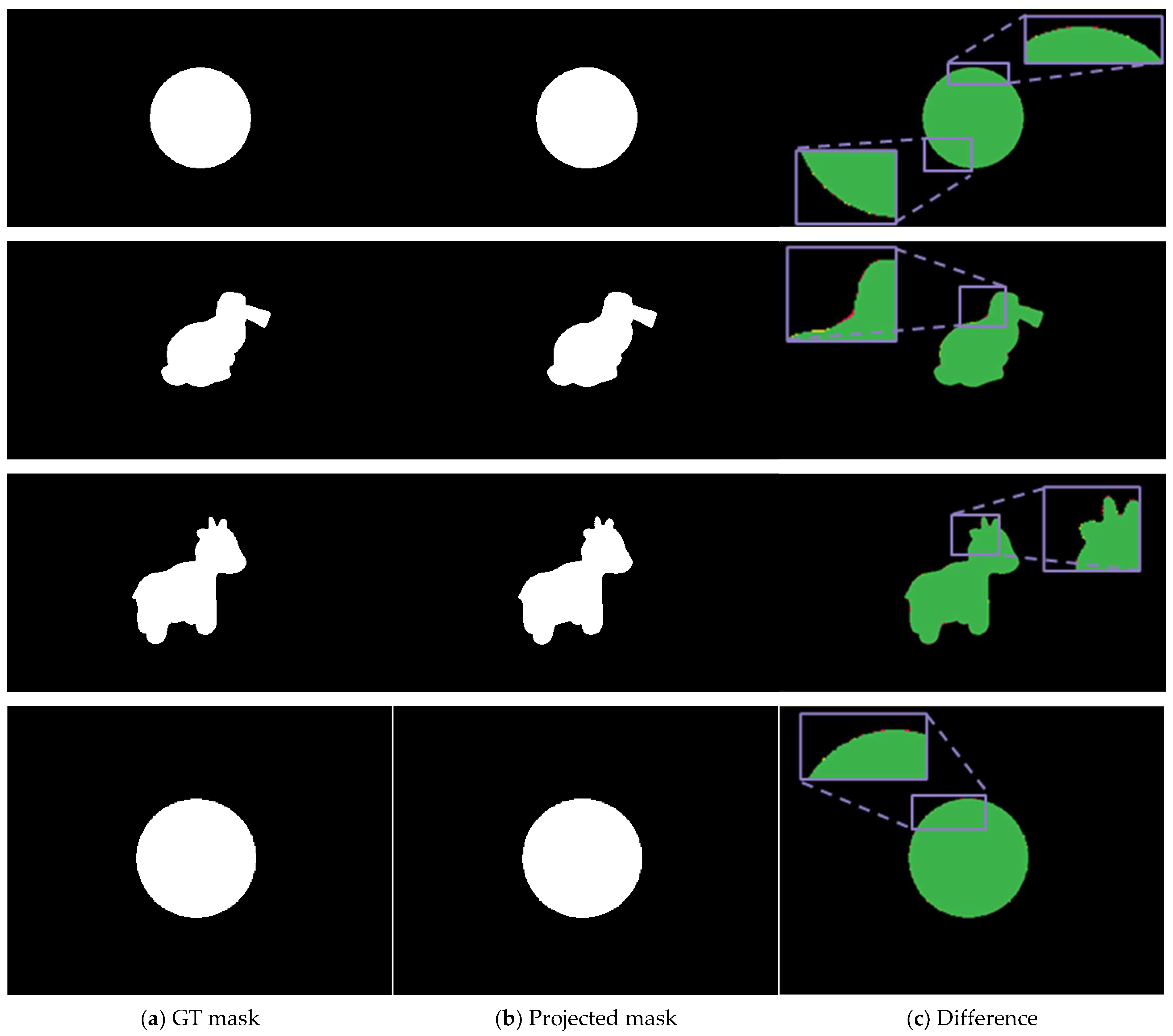
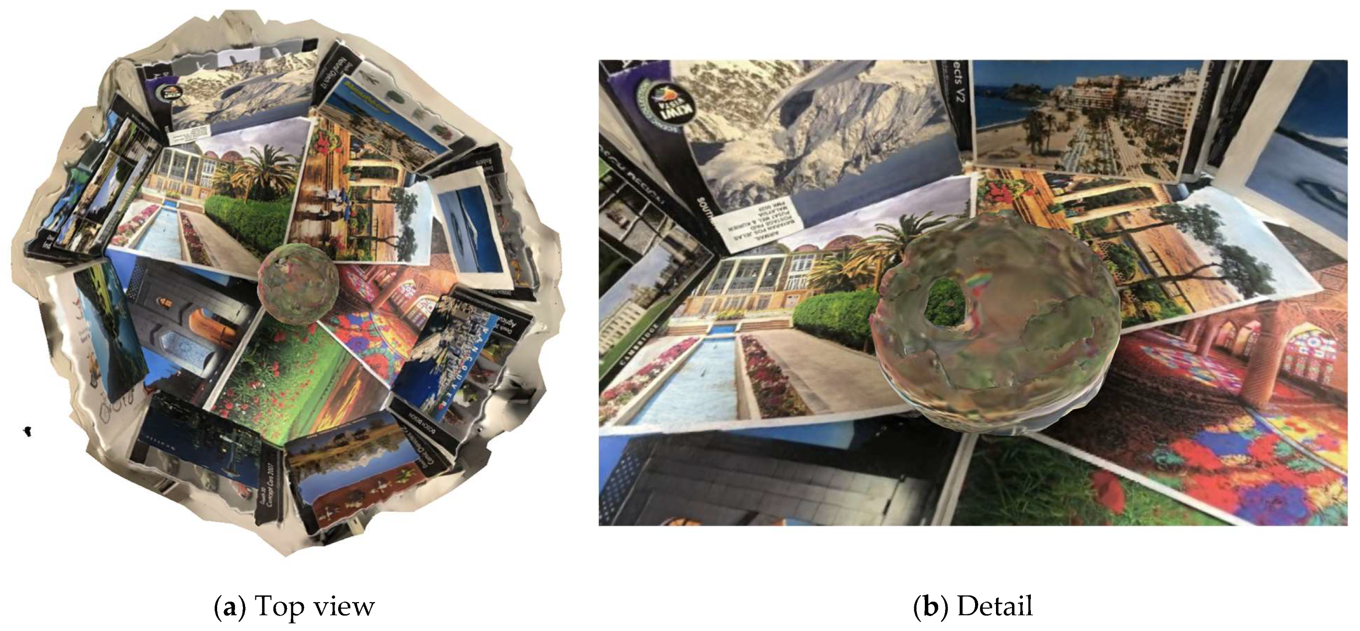
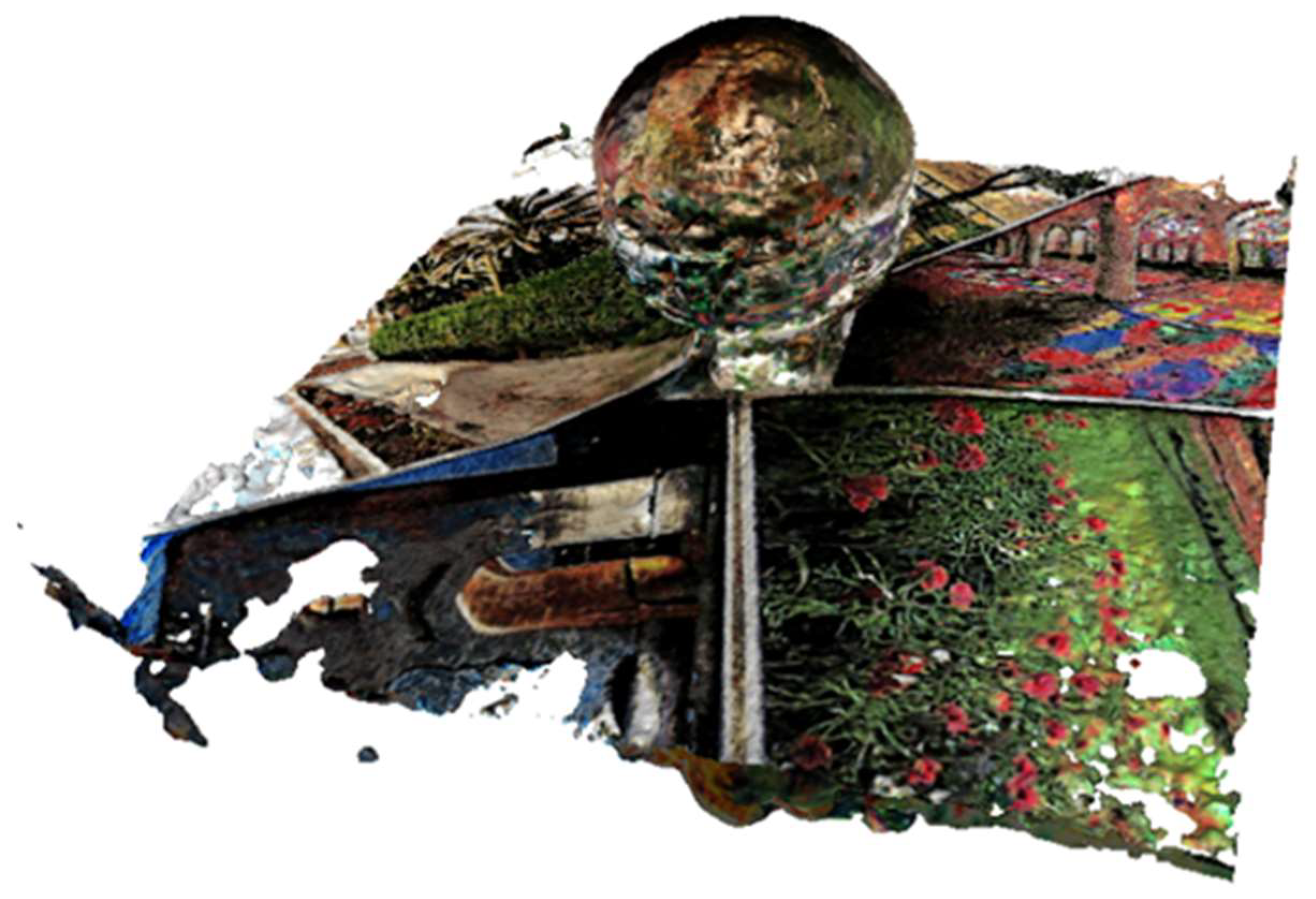
3.2.1. Geometric Reconstruction Results

The reconstruction results of transparent objects in different datasets are shown in Figure 8. Qualitatively, the surface geometric reconstruction based on DMTet achieved relatively stable effects on different datasets. Meanwhile, the geometric reconstruction algorithm based solely on the mask has relatively low requirements for input data, and the mask is not affected by refraction and reflection, which improves the practicability of the algorithm. Despite a deviation in several pixels at the edges of the mask that we extracted, we were still able to obtain reliable reconstruction results.

Due to the lack of geometric ground truth, we cannot directly evaluate the accuracy of mesh reconstruction. There are some quantitative evaluation methods for mesh quality without ground truth reference [54,55]. To adapt to the requirements of our method, we have designed an indirect quantitative evaluation approach. The projection of the reconstructed mesh under the camera poses can be obtained. We compared the projected mask with the manually refined ground truth mask in the test set and used Intersection over Union (IoU) as the evaluation metric.

Table 1. Pixel-level IoU between the ground truth and predicted mask for different scenes.

Datasets	Ball	Bunny	Cow	Glass
IoU	0.995	0.984	0.987	0.994

provides the IoU values for the test set across different scenes, demonstrating that our algorithm is capable of generating accurate meshes. We also show visual results of the ground truth mask, predicted mask, and the differences between them in Figure 9. We see that the mesh reconstructed using our algorithm can still produce generally correct projection results on the test set.

To compare the effect of our method in surface reconstruction, we use the mature commercial software, Metashape [53], to conduct 3D reconstruction on the glass scene, as shown in Figure 10. Since the ground truth is lacking, we only make a qualitative comparison. Apparently, refractive property of the glass causes the positions of the corresponding points in the foreground to change with the view, resulting in the failure of feature matching and model fitting.

We also applied NeuS, a relatively advanced geometry reconstruction algorithm based on deep learning, to reconstruct the glass dataset, as shown in Figure 11. Refraction makes the network learn the wrong SDF, resulting in holes and color errors on the object’s surface.

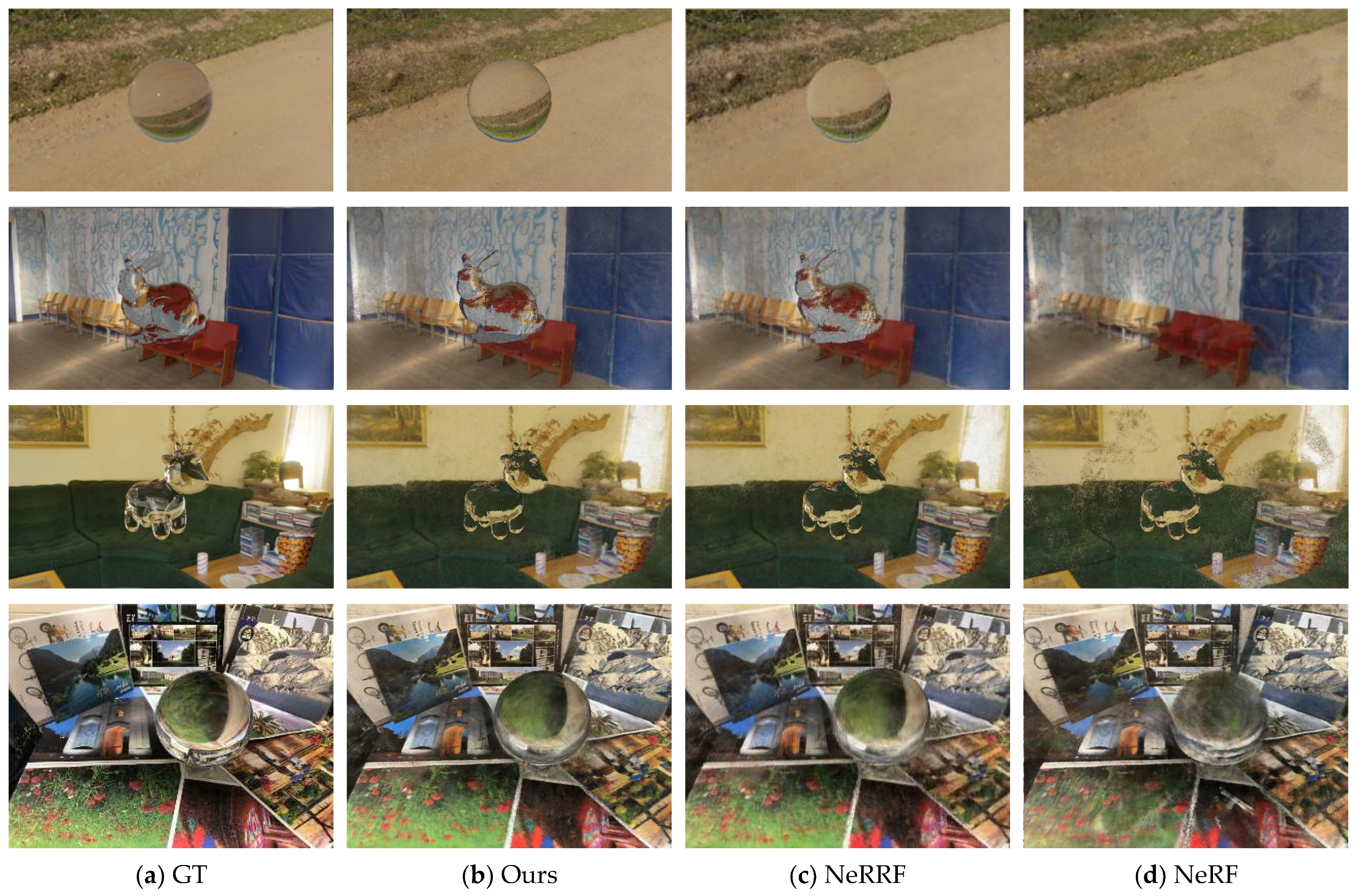
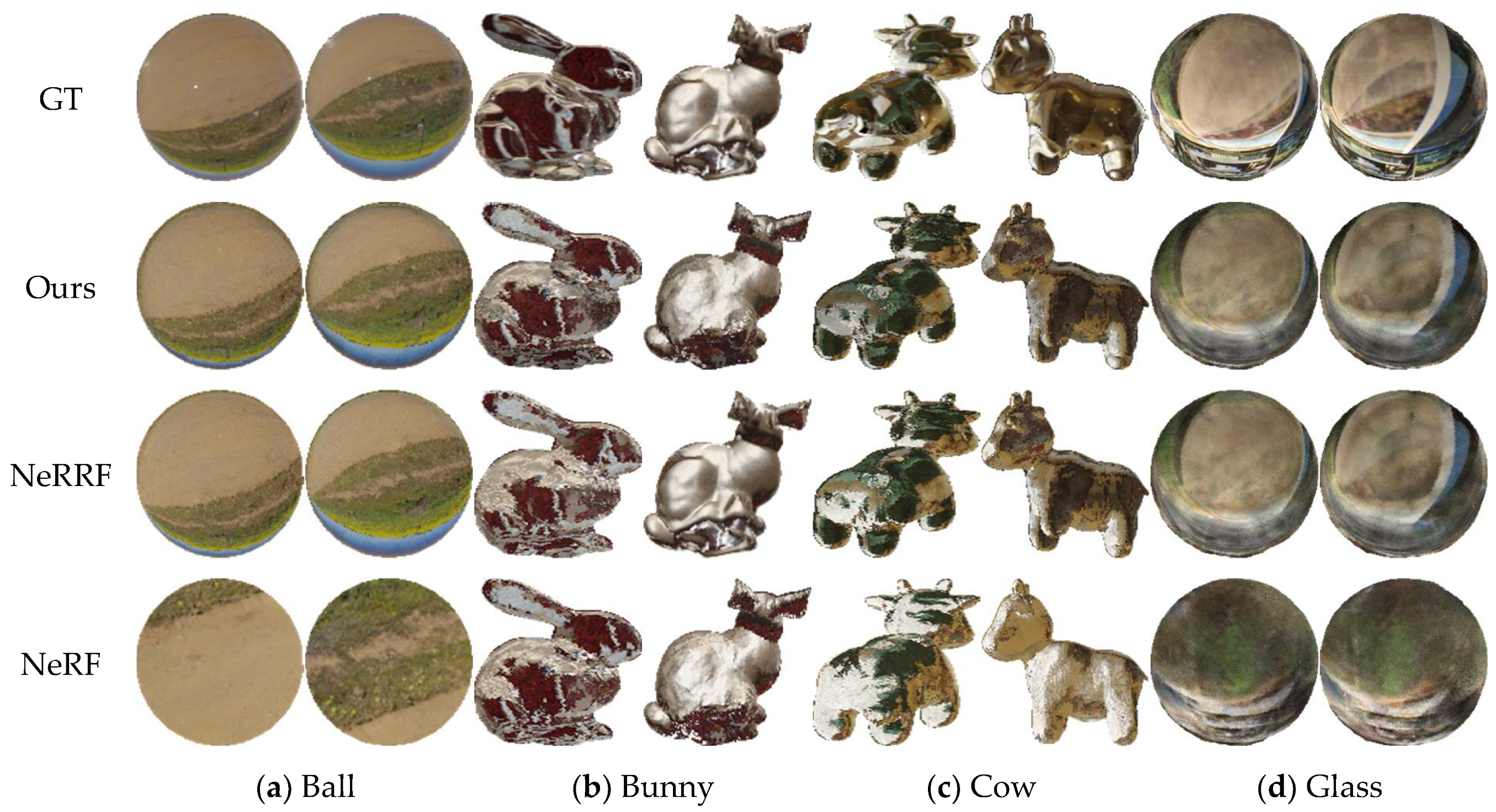
3.2.2. Results of Novel View Synthesis and IOR Optimization

Accurate geometric reconstruction supports us in executing reconstruction of the radiance field. We tested the effect of the proposed method in a novel view synthesis task on the test sets of the Blender dataset and the real-scene dataset and compared it with the Instant-NGP method.

Figure 12 provides a qualitative comparison among NeRF, the original NeRRF, our method, and the ground truth. To accelerate training and inference and improve the effect of novel view synthesis, we also adopted Instant-NGP for position encoding in NeRF. NeRF has a large deviation in radiance field training on the dataset of transparent objects due to refraction. Specifically, artifacts appear at multiple incorrect positions on the transparent objects. This is because the network wrongly learns the radiance field in that direction due to the refraction of light rays. In contrast, NeRRF and the method in this paper effectively avoid this problem.

We compared the results between the foreground detail of ground truth, our method, NeRRF, and NeRF, as illustrated in Figure 13. Our model effectively models the refraction phenomenon and achieves a realistic rendering effect. Due to the incorrect light modeling, NeRF learned the wrong distribution of the radiance field, resulting in severe blurring and position distortion on the object’s surface. In the ball and bunny datasets, NeRF could not even restore the foreground objects. In the cow dataset, incorrect ray directions caused NeRF to learn the wrong radiance fields, making artifacts of transparent objects appear in the background. In the glass datasets, NeRF had serious blurring on the surfaces of transparent objects.

Meanwhile, our method outperforms NeRRF in modeling the phenomenon of foreground darkening, especially at the edge parts. This is because we used a more accurate calculation formula for the radiance in ray tracing. This effect is quantitatively presented in

Table 2. Quantitative results on Blender the dataset for NeRF [52], NeRRF [47], NeRFRO [45], and ours. Comp. represents the results calculated using complete images (Complete Image), and Forg. represents the results calculated using foreground Images. The top three metrics are marked with gold, silver, and bronze. $\uparrow$: Larger values indicate better results; $\downarrow$: Smaller values are preferred.

Methods	$\mathbf{PSNR}\uparrow$		$\mathbf{SSIM}\uparrow$		$\mathbf{LPIPS}\downarrow$
	Comp.	Forg.	Comp.	Forg.	Comp.	Forg.
NeRF [52]	23.63	17.35	0.752	0.276	0.202	0.091
NeRRF [47]	26.72	17.53	0.830	0.404	0.123	0.092
NeRFRO 1 [45]	23.77	—	0.756	—	0.379	—
Ours	27.14	18.20	0.830	0.408	0.121	0.092

¹ The experimental data are from the work of [47].

. The comparison includes the complete image (Comp.) and the foreground image (Forg.). Our method, with the help of ray tracing, has achieved a far greater advantage over NeRF. Compared to vanilla NeRRF, our method does not require the prior knowledge of the initial IOR. This enables our method to be applied in scenes with transparent objects of any unknown materials.

Quantitative results on the glass dataset are summarized in

Table 3. Quantitative results on the glass dataset for NeRF [52], NeRRF [47], Mip-NeRF [25], NeRFRO [45], Eikonal [44], and our method. The top three metrics are marked with gold, silver, and bronze. $\uparrow$: Larger values indicate better results; $\downarrow$: Smaller values are preferred.

Methods	$\mathbf{PSNR}\uparrow$		$\mathbf{SSIM}\uparrow$		$\mathbf{LPIPS}\downarrow$
	Comp.	Forg.	Comp.	Forg.	Comp.	Forg.
NeRF [52]	16.90	14.00	0.505	0.254	0.313	0.211
NeRRF [47]	17.23	15.90	0.497	0.286	0.312	0.179
Mip-NeRF 1 [25]	16.29	—	0.523	—	0.418	—
NeRFRO 1 [45]	17.62	—	0.491	—	0.275	—
Eikonal 1 [44]	18.38	—	0.583	—	0.239	—
Ours	17.19	15.57	0.497	0.288	0.312	0.183

¹ The experiment data are from the work of [45].

. We compared our method with some relatively advanced algorithms currently available. The comparison includes the complete image and the foreground. Our evaluation reveals that our method is also comparable in terms of metrics.

Thanks to our IOR-adaptive algorithm, we can still obtain relatively accurate IORs. The comparison between the estimated IOR and the real IOR is shown in

Table 4. A quantitative comparison between the ground truth (GT) of IOR and the predicted values of our method.

Datasets	Ball	Bunny	Cow	Glass
IOR-GT	1.30	1.20	1.20	1.50
IOR-predicted	1.31	1.15	1.19	1.47

. The experiments demonstrate that our IOR estimation algorithm proposed in this paper can obtain a relatively accurate IOR, and the IOR that maximizes the foreground PSNR is selected. Although the IOR may deviate slightly, the rendering effect is still guaranteed.

Table 5. A quantitative comparison between our mask-based ray tracing and vanilla ray tracing in training and rendering. $\uparrow$: Larger values indicate better results; $\downarrow$: Smaller values are preferred.

	Ball		Bunny		Cow		Glass
	Training Time↓	$\mathbf{FPS}\uparrow$	Training Time↓	$\mathbf{FPS}\uparrow$	Training Time↓	$\mathbf{FPS}\uparrow$	Training Time↓	$\mathbf{FPS}\uparrow$
Complete	5 h 07 min	0.008	5 h 42 min	0.007	4 h 55 min	0.007	18 h 03 min	0.003
Mask-Based (Ours)	1 h 45 min	0.033	1 h 33 min	0.029	1 h 21 min	0.030	7 h 49 min	0.011

illustrates the quantitative speed comparison between our mask-based ray tracing and vanilla complete image ray tracing in training and rendering. Calculating the intersection of each pixel’s ray and mesh is a time-consuming operation. Our method effectively avoids the meaningless operation of the intersection between a large number of background pixels and mesh, which greatly improves the training speed and rendering speed.

To evaluate the effectiveness of the IOR optimization module and the new color calculation equation we introduced, we conducted ablation experiments. We incrementally added the IOR optimization module and the new color calculation equation during training. When the optimization is not applied, an IOR must be specified for training. To simulate the scenario without prior knowledge of the IOR, we subtracted 0.2 from the ground truth IOR and used this value for training.

The quantitative impact of different components on the synthetic dataset is shown in

Table 6. Novel view synthesis quality impacts of disabling various algorithm components on the synthetic dataset. $\uparrow$: Larger values indicate better results; $\downarrow$: Smaller values are preferred.

Methods	$\mathbf{PSNR}\uparrow$		$\mathbf{SSIM}\uparrow$		$\mathbf{LPIPS}\downarrow$
	Comp.	Forg.	Comp.	Forg.	Comp.	Forg.
Full Model	27.14	18.20	0.830	0.408	0.121	0.092
w/o Physical Constraints	26.64	17.14	0.811	0.385	0.129	0.097
w/o IOR Optimization	23.28	13.26	0.783	0.319	0.173	0.137

, and its impact on the real dataset is shown in

Table 7. Novel view synthesis quality impacts of disabling various algorithm components on the real dataset. $\uparrow$: Larger values indicate better results; $\downarrow$: Smaller values are preferred.

Methods	$\mathbf{PSNR}\uparrow$		$\mathbf{SSIM}\uparrow$		$\mathbf{LPIPS}\downarrow$
	Comp.	Forg.	Comp.	Forg.	Comp.	Forg.
Full Model	17.19	15.57	0.497	0.288	0.312	0.183
w/o Physical Constraints	17.11	15.28	0.487	0.272	0.332	0.239
w/o IOR Optimization	17.04	13.07	0.461	0.212	0.344	0.252

. The experiments demonstrate the effectiveness of our method, particularly in the foreground, where the addition of the two steps significantly improves the novel view synthesis.

The visual impact is illustrated in Figure 14. When the refractive index is unknown and not optimized, training the refractive radiance field leads to severe distortion in foreground colors and also affects the accuracy of the background radiance field due to incorrect light propagation paths. The color calculation formula we employ can more accurately model the darkening effect caused by refraction in the foreground, especially at the edges where the incident angle is large, causing the refraction phenomenon to disappear and making the edge part dark.

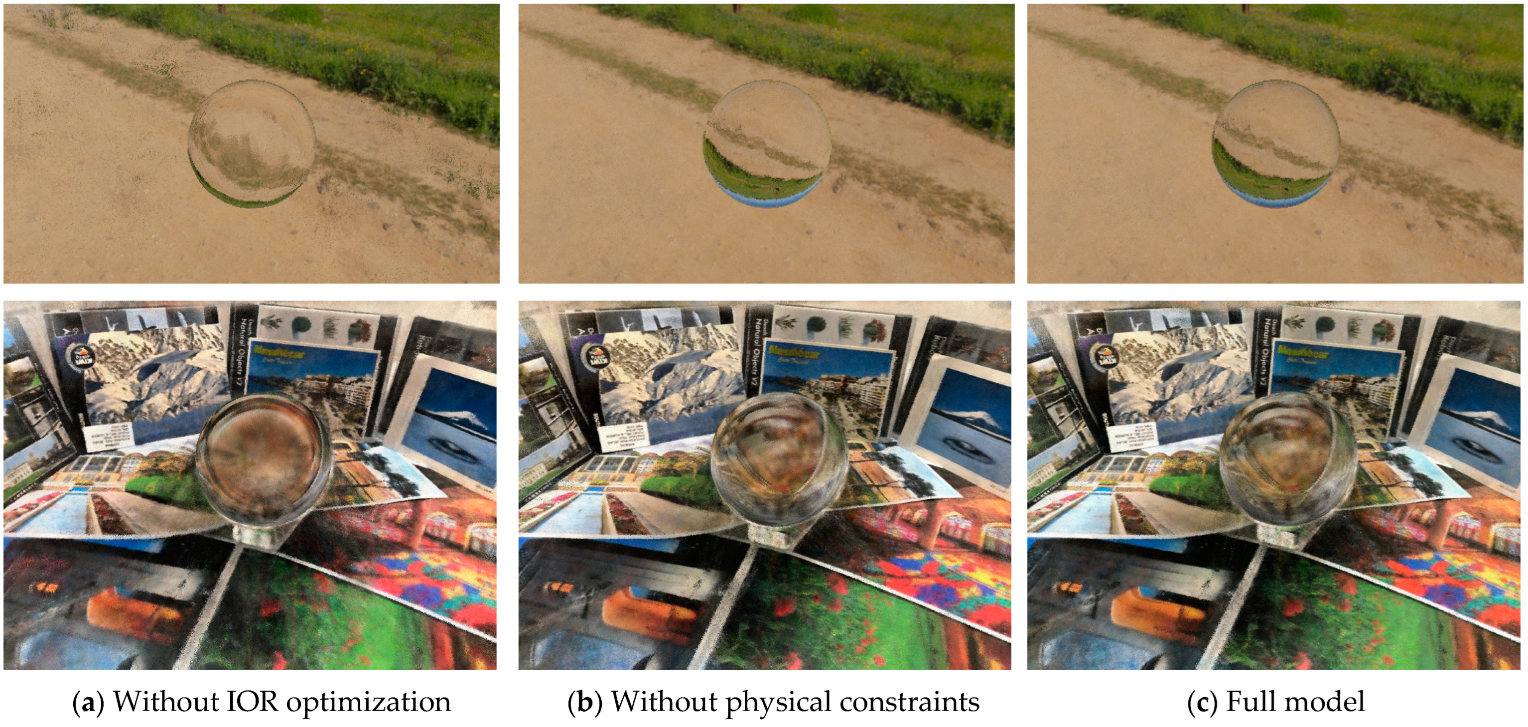
3.2.3. Supplementary Experiments

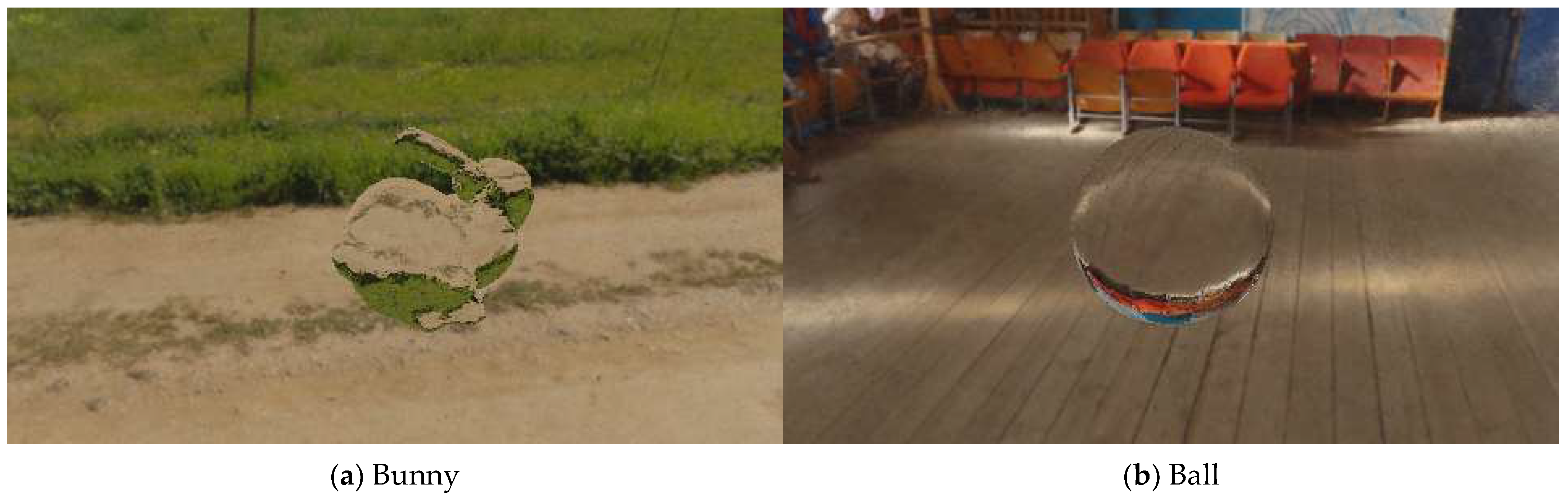
In addition to the novel view synthesis, since our method can obtain the environmental radiance field and object geometry, it can also perform scene editing, including object replacement and relighting. The results of ambient light estimation are given in Figure 15. Our method relatively accurately reconstructs the ambient light of the visible light paths in the dataset. The poor reconstruction effect of the upper ambient light is mainly due to the limitation of the views in the dataset. There is no upward shooting view in these datasets.

Thanks to our decoupling of object geometry and ambient light, we can edit scenes, as shown in Figure 16. These operations can be regarded as either object replacement under the existing ambient light or relighting of the existing objects.

Meanwhile, we can also modify the IOR. We demonstrate the IOR editing results of the ball dataset in Figure 17. Our method relatively accurately reconstructs the complete radiance field and decouples the radiance field from the IOR, making it possible to edit the IOR of the object. When the IOR is 1, transparent objects can be regarded as air, and no refraction phenomenon will occur. As the IOR increases, the refraction phenomenon gradually becomes more obvious, presenting more backgrounds in other directions. And when the IOR is set to 1.3, which is equal to the real IOR, the rendering image closest to GT is obtained.

4. Discussion

Using experiments on different datasets, we verified the effectiveness of our method. Our method enables high-quality novel view syntheses in various scenes. And no prior knowledge of IOR is required. Our method achieves more accurate refraction effect rendering, especially in the boundary part, using more accurate color calculations. Mask-based ray tracing greatly accelerates training and reasoning. In addition, we also tested ambient light reconstruction, scene editing, and refractive index editing. Experiments show that our method completely decouples all optical elements in the scene and can play a role in different tasks downstream.

5. Conclusions

We introduced an IOR-adaptive neural refractive radiance field. This algorithm consists of three main steps: geometric reconstruction, radiance field training, and IOR optimization. It can achieve novel view synthesis and IOR estimation without prior knowledge of the IOR. Based on retaining the characteristics of NeRRF, this algorithm realizes the adaptive optimization of the IOR and is comparable to the current best methods in terms of metrics. Meanwhile, our method has a foreground rendering effect that more conforms to the physical process and a faster rendering speed. It can be conveniently applied to numerous fields.

Table 8. A comparison of our proposed method to several recent novel view synthesis methods.

Methods	No Human Intervention?	No Additional Input?	Scene Editing OK?	Nested Objects OK?
NeRF [52]	√	√	×	×
NeRRF [47]	√	√	●	√
Nu-NeRF [46]	×	√	√	√
NeRFRO [45]	√	√	×	√
Eikonal [44]	√	×	×	√
Ours	●	√	√	×

shows a comparison of the characteristics of the different algorithms. No human intervention means that no human intervention is required during the execution process of the method. No additional input represents whether the method can complete reconstruction and novel view synthesis using only images as the initial data. Scene Editing OK represents whether the degree of scene reconstruction supports the editing of elements such as lighting and objects. Nested objects OK represents whether the reconstruction of nested objects is supported. √ represents full compliance, ● represents almost compliance, and × represents complete non-compliance. Our method has certain advantages in applicability compared to other methods.

Meanwhile, our method has some limitations. Because of the lack of strict geometric supervision, some errors were introduced during the process of surface reconstruction. These errors cause relatively large deviations in ray tracing for some pixels in the foreground and bring some rendering noise. Meanwhile, simple two-step ray tracing can hardly model the diffuse reflection properties and specular highlights of objects.

In the future, one possible improvement is to optimize geometric estimation and radiance field estimation simultaneously. In addition, investigating different radiance fields, including variations in lighting intensity and distance, particularly the impact of well-calibrated real-world radiance fields on the effectiveness of our method, remains to be explored. For the background radiance field, more powerful radiance field representation methods, such as Mip-NeRF, Zip-MeRF [56], etc., can be adopted. Finally, more accurate ray tracing inside the object can be added to achieve the reconstruction and rendering of nested objects and colored transparent objects.

References

1. Zhuang, S.F.; Tu, D.W.; Zhang, X. Research on Corresponding Point Matching and 3D Reconstruction of Underwater Binocular Stereo Vision. Chin. J. Sci. Instrum. 2022, 43, 147–154. [Google Scholar]
2. Weinmann, M.; Klein, R. Advances in Geometry and Reflectance Acquisition (Course Notes). In Proceedings of the SIGGRAPH Asia 2015 Courses, Kobe, Japan, 2–6 November 2015; pp. 1–71. [Google Scholar]
3. Zhang, Z.; Liu, X.; Guo, Z.; Gao, N.; Meng, X. Shape Measurement of Specular/Diffuse Complex Surface Based on Structured Light. Infrared Laser Eng. 2020, 49, 0303015. [Google Scholar] [CrossRef]
4. Bai, X.F.; Zhang, Z.H. 3D Shape Measurement Based on Colour Fringe Projection Techniques. Chin. J. Sci. Instrum. 2017, 38, 1912–1925. [Google Scholar]
5. Huang, S.; Shi, Y.; Li, M.; Qian, J.; Xu, K. Underwater 3D Reconstruction Using a Photometric Stereo with Illuminance Estimation. Appl. Opt. 2023, 62, 612–619. [Google Scholar] [CrossRef]
6. Aberman, K.; Katzir, O.; Zhou, Q.; Luo, Z.; Sharf, A.; Greif, C.; Chen, B.; Cohen-Or, D. Dip Transform for 3D Shape Reconstruction. ACM Trans. Graph. (TOG) 2017, 36, 1–11. [Google Scholar] [CrossRef]
7. Trifonov, B.; Bradley, D.; Heidrich, W. Tomographic Reconstruction of Transparent Objects. In ACM SIGGRAPH 2006 Sketches; Association for Computing Machinery: New York, NY, USA, 2006; pp. 55–es. [Google Scholar]
8. Hullin, M.B.; Fuchs, M.; Ihrke, I.; Seidel, H.-P.; Lensch, H. Fluorescent Immersion Range Scanning. In Proceedings of the ACM SIGGRAPH 2008, Los Angeles, CA, USA, 11–15 August 2008; ACM: New York, NY, USA, 2008; pp. 87.1–87.10. [Google Scholar]
9. Baihe, Q.; Yang, Q.; Xinyang, X.U. Surface Profile Reconstruction of Inhomogeneous Object Based on Direct Light Path Method. J. Chang. Univ. Sci. Technol. (Nat. Sci. Ed.) 2018, 41, 33–36+51. [Google Scholar]
10. Ji, Y.; Xia, Q.; Zhang, Z. Fusing Depth and Silhouette for Scanning Transparent Object with RGB-D Sensor. Int. J. Opt. 2017, 2017, 9796127. [Google Scholar] [CrossRef]
11. He, K.; Sui, C.; Huang, T.; Dai, R.; Lyu, C.; Liu, Y.-H. 3D Surface Reconstruction of Transparent Objects Using Laser Scanning with LTFtF Method. Opt. Lasers Eng. 2022, 148, 106774. [Google Scholar] [CrossRef]
12. Eren, G.; Aubreton, O.; Meriaudeau, F.; Sanchez Secades, L.A.; Fofi, D.; Teoman Naskali, A.; Truchetet, F.; Ercil, A. Scanning from Heating: 3D Shape Estimation of Transparent Objects from Local Surface Heating. Opt. Express 2009, 17, 11457–11468. [Google Scholar] [CrossRef]
13. Meriaudeau, F.; Secades, L.A.S.; Eren, G.; Erçil, A.; Truchetet, F.; Aubreton, O.; Fofi, D. 3-D Scanning of Nonopaque Objects by Means of Imaging Emitted Structured Infrared Patterns. IEEE Trans. Instrum. Meas. 2010, 59, 2898–2906. [Google Scholar] [CrossRef]
14. Rantoson, R.; Stolz, C.; Fofi, D.; Meriaudeau, F. Optimization of Transparent Objects Digitization from Visible Fluorescence Ultraviolet Induced. Opt. Eng. 2012, 51, 033601. [Google Scholar] [CrossRef]
15. Kutulakos, K.N.; Steger, E. A Theory of Refractive and Specular 3D Shape by Light-Path Triangulation. Int. J. Comput. Vis. 2008, 76, 13–29. [Google Scholar] [CrossRef]
16. Atcheson, B.; Ihrke, I.; Heidrich, W.; Tevs, A.; Bradley, D.; Magnor, M.; Seidel, H.-P. Time-Resolved 3D Capture of Non-Stationary Gas Flows. ACM Trans. Graph. (TOG) 2008, 27, 1–9. [Google Scholar] [CrossRef]
17. Wu, B. Image-based Modeling and Rendering of Transparent Objects. Doctoral Thesis, University of Chinese Academy of Sciences (Shenzhen Institutes of Advanced Technology Chinese Academy of Sciences), Shenzhen, China, 2019. [Google Scholar]
18. Hao, Z.; Liu, Y. Transparent Object Shape Measurement Based on Deflectometry. Proceedings 2018, 2, 548. [Google Scholar] [CrossRef]
19. Zongker, D.E.; Werner, D.M.; Curless, B.; Salesin, D.H. Environment Matting and Compositing. In Seminal Graphics Papers: Pushing the Boundaries; University of Washington: Seattle, WA, USA, 2023; Volume 2, pp. 537–546. [Google Scholar]
20. Chuang, Y.-Y.; Zongker, D.E.; Hindorff, J.; Curless, B.; Salesin, D.H.; Szeliski, R. Environment Matting Extensions: Towards Higher Accuracy and Real-Time Capture. In Proceedings of the 27th Annual Conference on Computer Graphics and Interactive Techniques, New York, NY, USA, July 23–28 2000; pp. 121–130. [Google Scholar]
21. Ihrke, I.; Kutulakos, K.N.; Lensch, H.P.; Magnor, M.; Heidrich, W. Transparent and Specular Object Reconstruction. In Proceedings of the Computer Graphics Forum; Wiley Online Library: Hoboken, NJ, USA, 2010; Volume 29, pp. 2400–2426. [Google Scholar]
22. Xu, X.; Lin, Y.; Zhou, H.; Zeng, C.; Yu, Y.; Zhou, K.; Wu, H. A Unified Spatial-Angular Structured Light for Single-View Acquisition of Shape and Reflectance. In Proceedings of the IEEE/CVF Conference on Computer Vision and Pattern Recognition, Vancouver, BC, Canada, 17–24 June 2023; pp. 206–215. [Google Scholar]
23. Liu, I.; Chen, L.; Fu, Z.; Wu, L.; Jin, H.; Li, Z.; Wong, C.M.R.; Xu, Y.; Ramamoorthi, R.; Xu, Z. Openillumination: A Multi-Illumination Dataset for Inverse Rendering Evaluation on Real Objects. Adv. Neural Inf. Process. Syst. 2024, 36, 36951–36962. [Google Scholar]
24. Mildenhall, B.; Srinivasan, P.P.; Tancik, M.; Barron, J.T.; Ramamoorthi, R.; Ng, R. Nerf: Representing Scenes as Neural Radiance Fields for View Synthesis. Commun. ACM 2021, 65, 99–106. [Google Scholar] [CrossRef]
25. Barron, J.T.; Mildenhall, B.; Tancik, M.; Hedman, P.; Martin-Brualla, R.; Srinivasan, P.P. Mip-Nerf: A Multiscale Representation for Anti-Aliasing Neural Radiance Fields. In Proceedings of the IEEE/CVF International Conference on Computer Vision, Paris, France, 1–6 October 2021; pp. 5855–5864. [Google Scholar]
26. Barron, J.T.; Mildenhall, B.; Verbin, D.; Srinivasan, P.P.; Hedman, P. Mip-Nerf 360: Unbounded Anti-Aliased Neural Radiance Fields. In Proceedings of the IEEE/CVF Conference on Computer Vision and Pattern Recognition, New Orleans, LA, USA, 18–24 June 2022; pp. 5470–5479. [Google Scholar]
27. Chen, Z.; Funkhouser, T.; Hedman, P.; Tagliasacchi, A. Mobilenerf: Exploiting the Polygon Rasterization Pipeline for Efficient Neural Field Rendering on Mobile Architectures. In Proceedings of the IEEE/CVF Conference on Computer Vision and Pattern Recognition, Vancouver, BC, Canada, 17–24 June 2023; pp. 16569–16578. [Google Scholar]
28. Qin, S.; Xiao, J.; Ge, J. Dip-NeRF: Depth-Based Anti-Aliased Neural Radiance Fields. Electronics 2024, 13, 1572. [Google Scholar] [CrossRef]
29. Srinivasan, P.P.; Deng, B.; Zhang, X.; Tancik, M.; Mildenhall, B.; Barron, J.T. Nerv: Neural Reflectance and Visibility Fields for Relighting and View Synthesis. In Proceedings of the IEEE/CVF Conference on Computer Vision and Pattern Recognition, Nashville, TN, USA, 20–25 June 2021; pp. 7495–7504. [Google Scholar]
30. Boss, M.; Jampani, V.; Braun, R.; Liu, C.; Barron, J.; Lensch, H. Neural-Pil: Neural Pre-Integrated Lighting for Reflectance Decomposition. Adv. Neural Inf. Process. Syst. 2021, 34, 10691–10704. [Google Scholar]
31. Jin, H.; Liu, I.; Xu, P.; Zhang, X.; Han, S.; Bi, S.; Zhou, X.; Xu, Z.; Su, H. Tensoir: Tensorial Inverse Rendering. In Proceedings of the IEEE/CVF Conference on Computer Vision and Pattern Recognition, Vancouver, BC, Canada, 17–24 June 2023; pp. 165–174. [Google Scholar]
32. Li, Z.; Wang, L.; Cheng, M.; Pan, C.; Yang, J. Multi-View Inverse Rendering for Large-Scale Real-World Indoor Scenes. In Proceedings of the IEEE/CVF Conference on Computer Vision and Pattern Recognition, Vancouver, BC, Canada, 17–24 June 2023; pp. 12499–12509. [Google Scholar]
33. Wang, P.; Liu, L.; Liu, Y.; Theobalt, C.; Komura, T.; Wang, W. Neus: Learning Neural Implicit Surfaces by Volume Rendering for Multi-View Reconstruction. arXiv 2021, arXiv:2106.10689. [Google Scholar]
34. Yao, Y.; Zhang, J.; Liu, J.; Qu, Y.; Fang, T.; McKinnon, D.; Tsin, Y.; Quan, L. Neilf: Neural Incident Light Field for Physically-Based Material Estimation. In Proceedings of the European Conference on Computer Vision, Tel Aviv, Israel, 23–27 October 2022; Springer: Berlin/Heidelberg, Germany, 2022; pp. 700–716. [Google Scholar]
35. Liu, Y.; Wang, P.; Lin, C.; Long, X.; Wang, J.; Liu, L.; Komura, T.; Wang, W. Nero: Neural Geometry and Brdf Reconstruction of Reflective Objects from Multiview Images. ACM Trans. Graph. (TOG) 2023, 42, 1–22. [Google Scholar] [CrossRef]
36. Zeng, C.; Chen, G.; Dong, Y.; Peers, P.; Wu, H.; Tong, X. Relighting Neural Radiance Fields with Shadow and Highlight Hints. In Proceedings of the ACM SIGGRAPH 2023 Conference Proceedings, Los Angeles, CA, USA, 6–10 August 2023; pp. 1–11. [Google Scholar]
37. Sainz, M.; Pajarola, R. Point-Based Rendering Techniques. Comput. Graph. 2004, 28, 869–879. [Google Scholar] [CrossRef]
38. Grossman, J.P.; Dally, W.J. Point Sample Rendering. In Proceedings of the Rendering Techniques’98: Proceedings of the Eurographics Workshop, Vienna, Austria, 29 June—1 July 1998; Springer: Berlin/Heidelberg, Germany, 1998; pp. 181–192. [Google Scholar]
39. Schütz, M.; Kerbl, B.; Wimmer, M. Software Rasterization of 2 Billion Points in Real Time. Proc. ACM Comput. Graph. Interact. Tech. 2022, 5, 1–17. [Google Scholar] [CrossRef]
40. Kerbl, B.; Kopanas, G.; Leimkühler, T.; Drettakis, G. 3D Gaussian Splatting for Real-Time Radiance Field Rendering. ACM Trans. Graph. 2023, 42, 1–14. [Google Scholar] [CrossRef]
41. Gao, J.; Gu, C.; Lin, Y.; Li, Z.; Zhu, H.; Cao, X.; Zhang, L.; Yao, Y. Relightable 3D Gaussians: Realistic Point Cloud Relighting with Brdf Decomposition and Ray Tracing. In Proceedings of the European Conference on Computer Vision, Paris, France, 26–27 March 2025; Springer: Berlin/Heidelberg, Germany, 2025; pp. 73–89. [Google Scholar]
42. Shi, Y.; Wu, Y.; Wu, C.; Liu, X.; Zhao, C.; Feng, H.; Liu, J.; Zhang, L.; Zhang, J.; Zhou, B. Gir: 3D Gaussian Inverse Rendering for Relightable Scene Factorization. arXiv 2023, arXiv:2312.05133. [Google Scholar]
43. Jiang, Y.; Tu, J.; Liu, Y.; Gao, X.; Long, X.; Wang, W.; Ma, Y. Gaussianshader: 3D Gaussian Splatting with Shading Functions for Reflective Surfaces. In Proceedings of the IEEE/CVF Conference on Computer Vision and Pattern Recognition, Seattle, WA, USA, 16–22 June 2024; pp. 5322–5332. [Google Scholar]
44. Bemana, M.; Myszkowski, K.; Revall Frisvad, J.; Seidel, H.-P.; Ritschel, T. Eikonal Fields for Refractive Novel-View Synthesis. In Proceedings of the ACM SIGGRAPH 2022 Conference Proceedings, Vancouver, BC, Canada, 7–11 August 2022; pp. 1–9. [Google Scholar]
45. Pan, J.-I.; Su, J.-W.; Hsiao, K.-W.; Yen, T.-Y.; Chu, H.-K. Sampling Neural Radiance Fields for Refractive Objects. In Proceedings of the SIGGRAPH Asia 2022 Technical Communications, Daegu, Republic of Korea, 6–9 December 2022; pp. 1–4. [Google Scholar]
46. Sun, J.-M.; Wu, T.; Yan, L.-Q.; Gao, L. NU-NeRF: Neural Reconstruction of Nested Transparent Objects with Uncontrolled Capture Environment. ACM Trans. Graph. (TOG) 2024, 43, 1–14. [Google Scholar] [CrossRef]
47. Chen, X.; Liu, J.; Zhao, H.; Zhou, G.; Zhang, Y.-Q. Nerrf: 3D Reconstruction and View Synthesis for Transparent and Specular Objects with Neural Refractive-Reflective Fields. arXiv 2023, arXiv:2309.13039. [Google Scholar]
48. Shen, T.; Gao, J.; Yin, K.; Liu, M.-Y.; Fidler, S. Deep Marching Tetrahedra: A Hybrid Representation for High-Resolution 3D Shape Synthesis. Adv. Neural Inf. Process. Syst. 2021, 34, 6087–6101. [Google Scholar]
49. Kirillov, A.; Mintun, E.; Ravi, N.; Mao, H.; Rolland, C.; Gustafson, L.; Xiao, T.; Whitehead, S.; Berg, A.C.; Lo, W.-Y. Segment Anything. In Proceedings of the IEEE/CVF International Conference on Computer Vision, Paris, France, 2–3 October 2023; pp. 4015–4026. [Google Scholar]
50. Schonberger, J.L.; Frahm, J.-M. Structure-from-Motion Revisited. In Proceedings of the IEEE Conference on Computer Vision and Pattern Recognition, Las Vegas, NV, USA, 27–30 June 2016; pp. 4104–4113. [Google Scholar]
51. Gropp, A.; Yariv, L.; Haim, N.; Atzmon, M.; Lipman, Y. Implicit Geometric Regularization for Learning Shapes. arXiv 2020, arXiv:2002.10099. [Google Scholar]
52. Müller, T.; Evans, A.; Schied, C.; Keller, A. Instant Neural Graphics Primitives with a Multiresolution Hash Encoding. ACM Trans. Graph. (TOG) 2022, 41, 1–15. [Google Scholar] [CrossRef]
53. Metashape. Available online: https://www.agisoft.com/ (accessed on 7 October 2023).
54. Sarvestani, A.S.; Zhou, W.; Wang, Z. Perceptual Crack Detection for Rendered 3D Textured Meshes. In Proceedings of the 2024 16th International Conference on Quality of Multimedia Experience (QoMEX), Karlshamn, Sweden, 18–20 June 2024; pp. 1–7. [Google Scholar]
55. Zhang, Z.; Sun, W.; Min, X.; Wang, T.; Lu, W.; Zhai, G. No-Reference Quality Assessment for 3D Colored Point Cloud and Mesh Models. IEEE Trans. Circuits Syst. Video Technol. 2022, 32, 7618–7631. [Google Scholar] [CrossRef]
56. Barron, J.T.; Mildenhall, B.; Verbin, D.; Srinivasan, P.P.; Hedman, P. Zip-Nerf: Anti-Aliased Grid-Based Neural Radiance Fields. In Proceedings of the IEEE/CVF International Conference on Computer Vision, Paris, France, 2–3 October 2023; pp. 19697–19705. [Google Scholar]
Figure 1. Framework of the refraction scene reconstruction method. The pipeline mainly includes five steps: (1) Mask extraction and sparse reconstruction. (2) Geometric reconstruction through the DMTet algorithm with masks and poses. (3) Background radiance field training. (4) Best IOR searching. (5) Complete radiance field training. Compared with NeRRF, our method adds the IOR optimization module (steps 3 and 4).
Electronics 14 01073 g001
Figure 2. Comparison chart between the Vanilla NeRF (orange), Eikonal NeRF (green), and the refraction NeRF (blue). The vanilla NeRF constraints ray propagates along a straight line [24], and Eikonal NeRF distorts the ray in each voxel, which does not conform to the real light path [44,45]. Our method calculates the real light path using ray tracing.
Electronics 14 01073 g002
Figure 3. Ray tracing of refraction and reflection. This method mainly includes (1) calculating the direction of reflection and refraction according to ray tracing. And (2) calculating the color of the corresponding pixel according to Fresnel’s law and the color weighting in the direction of reflection and refraction.
Electronics 14 01073 g003
Figure 4. Pipeline of IOR optimization.
Electronics 14 01073 g004
Figure 5. The dataset used to evaluate the methods.
Electronics 14 01073 g005
Figure 6. SAM mask extraction results. (a) Original image. (b) Schematic diagram of the foreground mask. For the convenience of display, the foreground retains the original image color and the background is set to black.
Electronics 14 01073 g006
Figure 7. The scene reconstructed using COLMAP. Camera poses of each image, as well as a sparse point cloud, are shown.
Electronics 14 01073 g007
Figure 8. Surface reconstruction results.
Electronics 14 01073 g008
Figure 9. Visualization of the (a) ground truth (GT) mask, (b) projected mask, and (c) their difference.
Electronics 14 01073 g009
Figure 10. Reconstruction results of the glass ball scene using Metashape.
Electronics 14 01073 g010
Figure 11. Reconstruction results of the glass ball scene using NeuS.
Electronics 14 01073 g011
Figure 12. A qualitative comparison from experiments on the Blender dataset and glass dataset for (a) GT, (b) ours, (c) NeRRF, and (d) NeRF on a novel view synthesis task.
Electronics 14 01073 g012
Figure 13. A qualitative comparison of the foreground rendering details of the (a) ball, (b) bunny, (c) cow, and (d) glass view synthesis tasks.
Electronics 14 01073 g013
Figure 14. Qualitative results on the effects of disabling various algorithm components.
Electronics 14 01073 g014
Figure 15. Ambient light reconstruction results.
Electronics 14 01073 g015
Figure 16. Results of ambient light editing and scene editing. (a) Bunny in the ambient light of the ball. (b) Ball in the ambient light of the bunny.
Electronics 14 01073 g016
Figure 17. Novel view synthesis results under different IORs.
Electronics 14 01073 g017