
LIME


Abstract
1. Introduction
- (i)
- define a multi-class explainability optimization objective;
- (ii)
- operationalize it in the form of a local surrogate;
- (iii)
- offer an algorithm for building multi-class explainers; and
- (iv)
- implement it with multi-output regression trees.
2. Related Work and Background
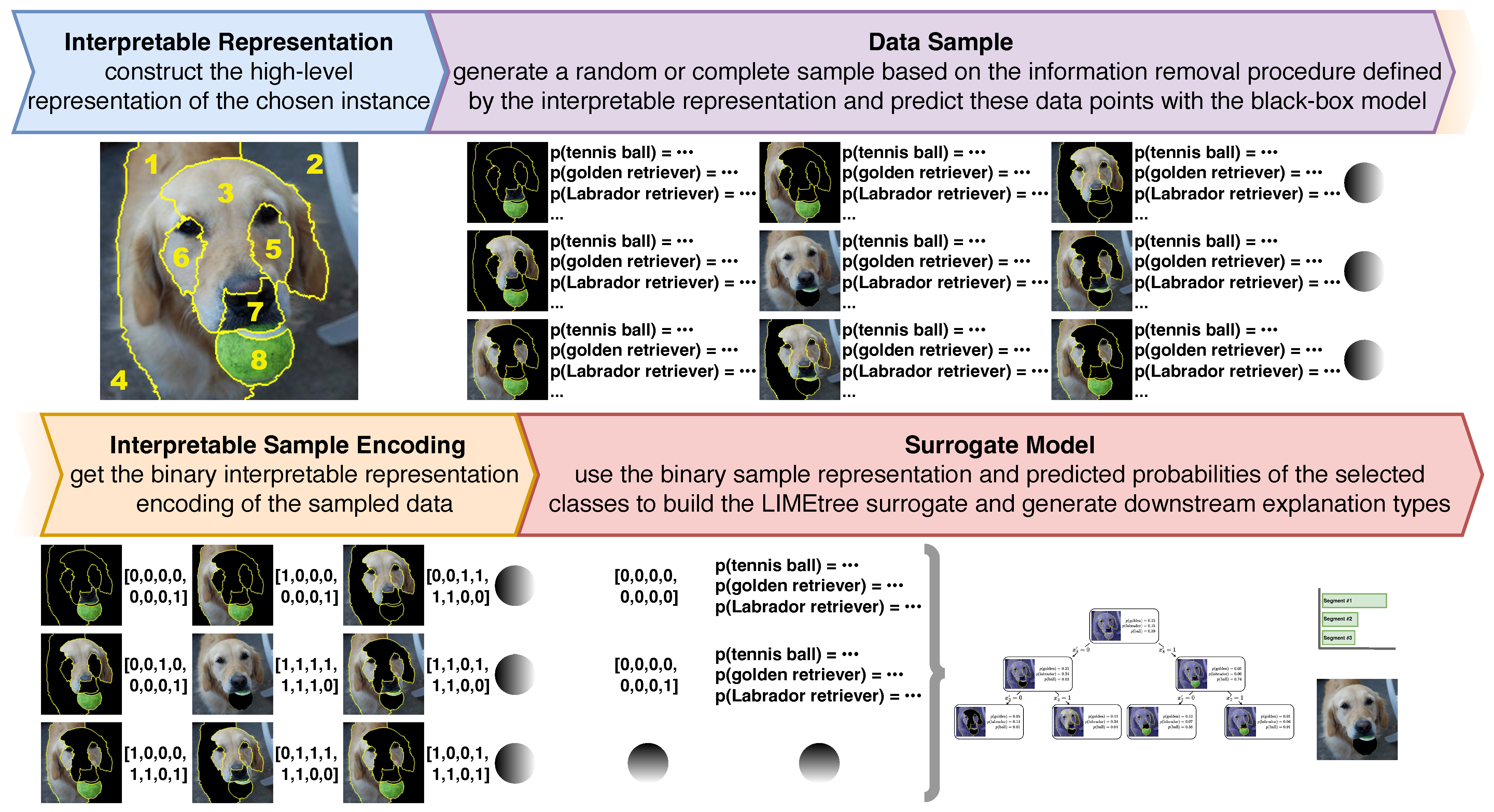
3. LIME
4. Fidelity Guarantees
5. Qualitative, Quantitative and User-Based Evaluation
5.1. Desiderata
5.2. Synthetic Experiments
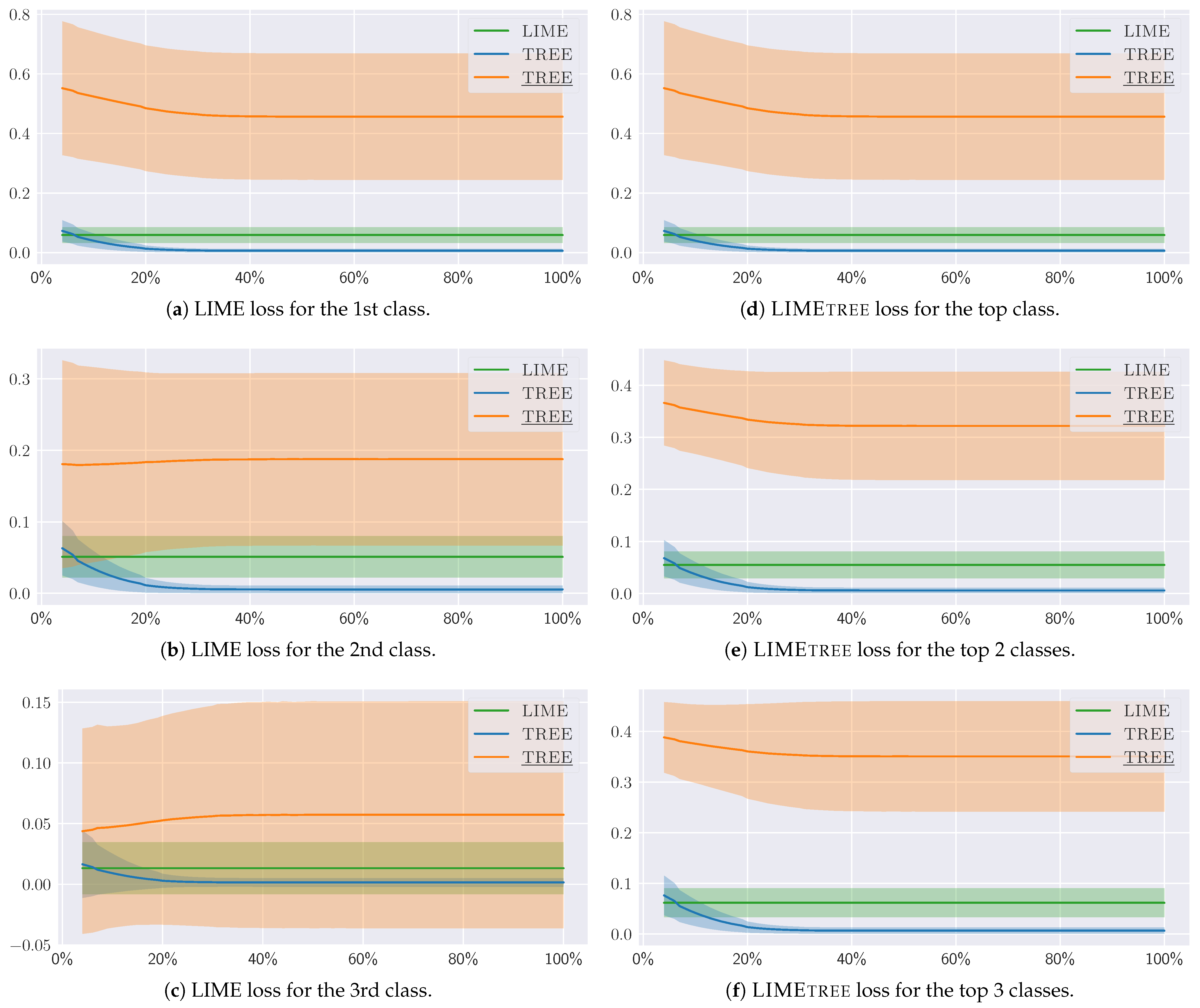
- TREE
- optimizes a surrogate tree for complexity, i.e., it determines the shallowest tree that offers the desired level of fidelity;
- TREE
- is a variant of TREE whose predictions are post-processed to guarantee full fidelity of model-driven explanations; and
- TREE †
- constructs a surrogate tree without any complexity constraints, allowing the algorithm to build a complete tree that guarantees full fidelity of both model- and data-driven explanations.
5.3. Pilot User Study
6. Discussion
7. Conclusions and Future Work
Author Contributions
Funding
Institutional Review Board Statement
Informed Consent Statement
Data Availability Statement
Acknowledgments
Conflicts of Interest
Abbreviations
| AI | Artificial Intelligence |
| CPU | Central Processing Unit |
| GAM | Generalized Additive Model |
| GPU | Graphics Processing Unit |
| IR | Interpretable Representation |
| LIME | Local Interpretable Model-agnostic Explanations |
| XAI | eXplainable Artificial Intelligence |
Appendix A. LIME Algorithms
| Algorithm A1: The TREE (vanilla) variant of LIME. |
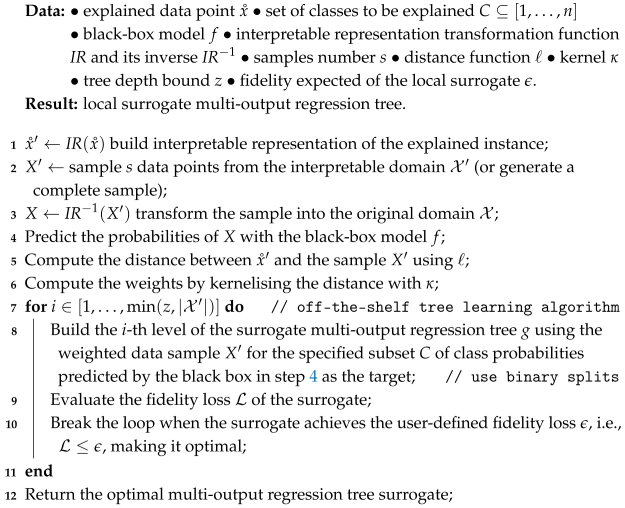 |
| Algorithm A2: The TREE variant of LIME. |
 |
Appendix B. Proofs
Appendix C. Loss Behavior


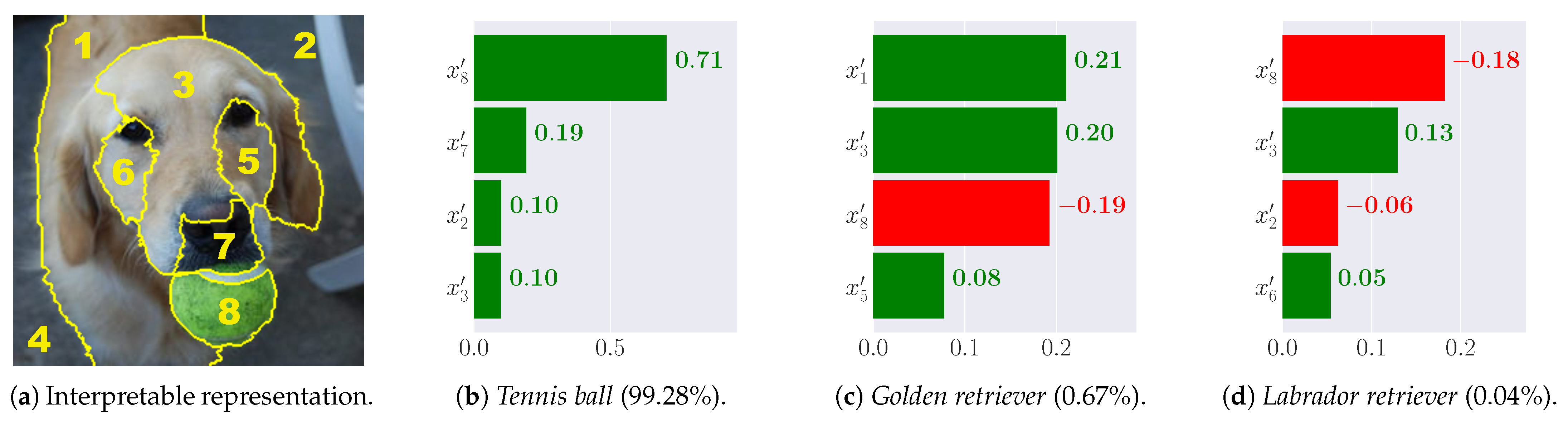
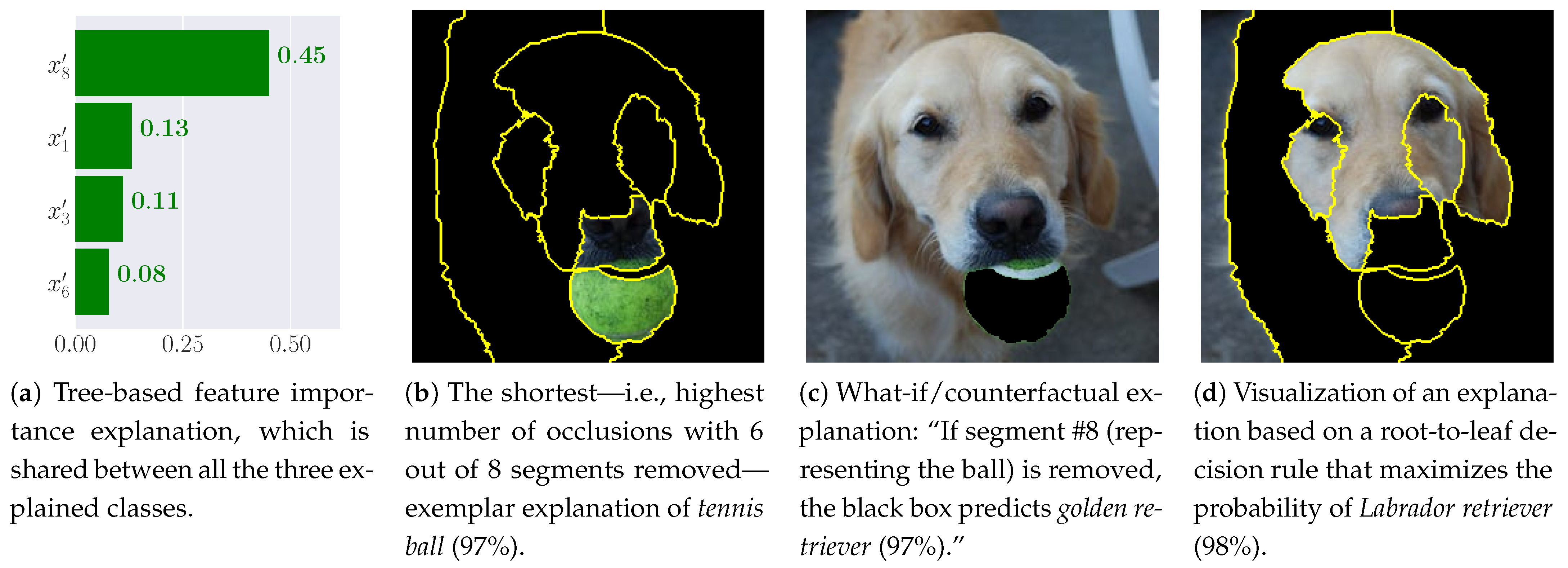
Appendix D. Examples of Diverse Explanation Types


References
- Rudin, C. Stop explaining black box machine learning models for high stakes decisions and use interpretable models instead. Nat. Mach. Intell. 2019, 1, 206–215. [Google Scholar] [CrossRef] [PubMed]
- Sokol, K.; Flach, P. Explainability is in the mind of the beholder: Establishing the foundations of explainable artificial intelligence. arXiv 2021, arXiv:2112.14466. [Google Scholar]
- Longo, L.; Brcic, M.; Cabitza, F.; Choi, J.; Confalonieri, R.; Del Ser, J.; Guidotti, R.; Hayashi, Y.; Herrera, F.; Holzinger, A.; et al. Explainable artificial intelligence (XAI) 2.0: A manifesto of open challenges and interdisciplinary research directions. Inf. Fusion 2024, 106, 102301. [Google Scholar] [CrossRef]
- Guidotti, R.; Monreale, A.; Ruggieri, S.; Turini, F.; Giannotti, F.; Pedreschi, D. A survey of methods for explaining black box models. ACM Comput. Surv. (CSUR) 2018, 51, 1–42. [Google Scholar] [CrossRef]
- Miller, T. Explanation in artificial intelligence: Insights from the social sciences. Artif. Intell. 2019, 267, 1–38. [Google Scholar] [CrossRef]
- Wachter, S.; Mittelstadt, B.; Russell, C. Counterfactual explanations without opening the black box: Automated decisions and the GPDR. Harv. J. Law Technol. 2017, 31, 841. [Google Scholar] [CrossRef]
- Poyiadzi, R.; Sokol, K.; Santos-Rodriguez, R.; De Bie, T.; Flach, P. FACE: Feasible and actionable counterfactual explanations. In Proceedings of the AAAI/ACM Conference on AI, Ethics, and Society, New York, NY, USA, 7–8 February 2020; pp. 344–350. [Google Scholar]
- Romashov, P.; Gjoreski, M.; Sokol, K.; Martinez, M.V.; Langheinrich, M. BayCon: Model-agnostic Bayesian counterfactual generator. In Proceedings of the IJCAI, Vienna, Austria, 23–29 July 2022; pp. 740–746. [Google Scholar]
- Waa, J.v.d.; Robeer, M.; Diggelen, J.v.; Brinkhuis, M.; Neerincx, M. Contrastive explanations with local foil trees. In Proceedings of the 2018 ICML Workshop on Human Interpretability in Machine Learning (WHI 2018), Stockholm, Sweden, 14 July 2018. [Google Scholar]
- Verma, S.; Boonsanong, V.; Hoang, M.; Hines, K.; Dickerson, J.; Shah, C. Counterfactual explanations and algorithmic recourses for machine learning: A review. ACM Comput. Surv. (CSUR) 2024, 56, 1–42. [Google Scholar] [CrossRef]
- Byrne, R.M. Good explanations in explainable artificial intelligence (XAI): Evidence from human explanatory reasoning. In Proceedings of the IJCAI, Macao, China, 19–25 August 2023; pp. 6536–6544. [Google Scholar]
- Miller, T. Explainable AI is dead, long live explainable AI! Hypothesis-driven decision support using evaluative AI. In Proceedings of the 2023 ACM Conference on Fairness, Accountability, and Transparency, Chicago, IL, USA, 12–15 June 2023; pp. 333–342. [Google Scholar]
- Weld, D.S.; Bansal, G. The challenge of crafting intelligible intelligence. Commun. ACM 2019, 62, 70–79. [Google Scholar] [CrossRef]
- Craven, M.; Shavlik, J.W. Extracting tree-structured representations of trained networks. In Proceedings of the Advances in Neural Information Processing Systems, Denver, CO, USA, 27–30 November 1995; pp. 24–30. [Google Scholar]
- Breiman, L.; Friedman, J.; Stone, C.J.; Olshen, R.A. Classification and Regression Trees; Chapman and Hall/CRC: New York, NY, USA, 1984. [Google Scholar]
- Sokol, K. Towards Intelligible and Robust Surrogate Explainers: A Decision Tree Perspective. Ph.D. Thesis, University of Bristol, Bristol, UK, 2021. [Google Scholar]
- Saeed, W.; Omlin, C. Explainable AI (XAI): A systematic meta-survey of current challenges and future opportunities. Knowl.-Based Syst. 2023, 263, 110273. [Google Scholar] [CrossRef]
- Retzlaff, C.O.; Angerschmid, A.; Saranti, A.; Schneeberger, D.; Roettger, R.; Mueller, H.; Holzinger, A. Post-hoc vs ante-hoc explanations: xAI design guidelines for data scientists. Cogn. Syst. Res. 2024, 86, 101243. [Google Scholar] [CrossRef]
- Karimi, A.; Schölkopf, B.; Valera, I. Algorithmic recourse: From counterfactual explanations to interventions. In Proceedings of the 2021 ACM Conference on Fairness, Accountability, and Transparency, Virtual Event, 3–10 March 2021; pp. 353–362. [Google Scholar]
- Sokol, K.; Flach, P. Explainability fact sheets: A framework for systematic assessment of explainable approaches. In Proceedings of the 2020 ACM Conference on Fairness, Accountability, and Transparency, Barcelona, Spain, 27–30 January 2020; pp. 56–67. [Google Scholar]
- Guidotti, R. Counterfactual explanations and how to find them: Literature review and benchmarking. Data Min. Knowl. Discov. 2024, 38, 2770–2824. [Google Scholar] [CrossRef]
- Meske, C.; Bunde, E.; Schneider, J.; Gersch, M. Explainable artificial intelligence: Objectives, stakeholders, and future research opportunities. Inf. Syst. Manag. 2022, 39, 53–63. [Google Scholar] [CrossRef]
- Ribeiro, M.T.; Singh, S.; Guestrin, C. “Why should I trust you?”: Explaining the predictions of any classifier. In Proceedings of the 22nd ACM SIGKDD International Conference on Knowledge Discovery and Data Mining, San Francisco, CA, USA, 13–17 August 2016; pp. 1135–1144. [Google Scholar]
- Sokol, K.; Hepburn, A.; Santos-Rodriguez, R.; Flach, P. bLIMEy: Surrogate prediction explanations beyond LIME. In Proceedings of the 2019 Workshop on Human-Centric Machine Learning (HCML 2019) at the 33rd Conference on Neural Information Processing Systems (NeurIPS 2019), Vancouver, BC, Canada, 13 December 2019. [Google Scholar]
- Sokol, K.; Flach, P. Interpretable representations in explainable AI: From theory to practice. Data Min. Knowl. Discov. 2024, 38, 1–39. [Google Scholar] [CrossRef]
- Sokol, K.; Hepburn, A.; Santos-Rodriguez, R.; Flach, P. What and how of machine learning transparency: Building bespoke explainability tools with interoperable algorithmic components. J. Open Source Educ. 2022, 5, 175. [Google Scholar] [CrossRef]
- Carlevaro, A.; Lenatti, M.; Paglialonga, A.; Mongelli, M. Multi-class counterfactual explanations using support vector data description. IEEE Trans. Artif. Intell. 2023, 5, 3046–3056. [Google Scholar] [CrossRef]
- Hastie, T.; Tibshirani, R. Generalized additive models. Stat. Sci. 1986, 1, 297–310. [Google Scholar] [CrossRef]
- Lou, Y.; Caruana, R.; Gehrke, J. Intelligible models for classification and regression. In Proceedings of the 18th ACM SIGKDD International Conference on Knowledge Discovery and Data Mining, Beijing, China, 12–16 August 2012; pp. 150–158. [Google Scholar]
- Zhang, X.; Tan, S.; Koch, P.; Lou, Y.; Chajewska, U.; Caruana, R. Axiomatic interpretability for multiclass additive models. In Proceedings of the 25th ACM SIGKDD International Conference on Knowledge Discovery and Data Mining, Anchorage, AK, USA, 4–8 August 2019; pp. 226–234. [Google Scholar]
- Shi, S.; Zhang, X.; Li, H.; Fan, W. Explaining the predictions of any image classifier via decision trees. arXiv 2019, arXiv:1911.01058. [Google Scholar]
- Tolomei, G.; Silvestri, F.; Haines, A.; Lalmas, M. Interpretable predictions of tree-based ensembles via actionable feature tweaking. In Proceedings of the 23rd ACM SIGKDD International Conference on Knowledge Discovery and Data Mining, Halifax, NS, Canada, 13–17 August 2017; pp. 465–474. [Google Scholar]
- Sokol, K.; Flach, P.A. Glass-Box: Explaining AI decisions with counterfactual statements through conversation with a voice-enabled virtual assistant. In Proceedings of the IJCAI, Stockholm, Sweden, 13–19 July 2018; pp. 5868–5870. [Google Scholar]
- Sokol, K.; Flach, P. One explanation does not fit all: The promise of interactive explanations for machine learning transparency. KI-KÜNstliche Intell. 2020, 34, 235–250. [Google Scholar] [CrossRef]
- Flach, P. Machine Learning: The Art and Science of Algorithms That Make Sense of Data; Cambridge University Press: Cambridge, UK, 2012. [Google Scholar]
- Breiman, L. Random forests. Mach. Learn. 2001, 45, 5–32. [Google Scholar] [CrossRef]
- Laugel, T.; Renard, X.; Lesot, M.J.; Marsala, C.; Detyniecki, M. Defining locality for surrogates in post-hoc interpretablity. In Proceedings of the 2018 ICML Workshop on Human Interpretability in Machine Learning (WHI 2018), Stockholm, Sweden, 14 July 2018. [Google Scholar]
- Zhang, Y.; Song, K.; Sun, Y.; Tan, S.; Udell, M. “Why should you trust my explanation?” Understanding uncertainty in LIME explanations. In Proceedings of the AI for Social Good Workshop at the 36th International Conference on Machine Learning (ICML 2019), Long Beach, CA, USA, 9–15 June 2019. [Google Scholar]
- Doshi-Velez, F.; Kim, B. Considerations for evaluation and generalization in interpretable machine learning. In Explainable and Interpretable Models in Computer Vision and Machine Learning; Springer: Cham, Switzerland, 2018; pp. 3–17. [Google Scholar]
- Sokol, K.; Vogt, J.E. What does evaluation of explainable artificial intelligence actually tell us? A case for compositional and contextual validation of XAI building blocks. In Proceedings of the Extended Abstracts of the 2024 CHI Conference on Human Factors in Computing Systems, Honolulu, HI, USA, 11–16 May 2024; pp. 1–8. [Google Scholar]
- Mittelstadt, B.; Russell, C.; Wachter, S. Explaining explanations in AI. In Proceedings of the 2019 ACM Conference on Fairness, Accountability, and Transparency, Atlanta, GA, USA, 29–31 January 2019; pp. 279–288. [Google Scholar]
- Sokol, K.; Vogt, J.E. (Un)reasonable allure of ante-hoc interpretability for high-stakes domains: Transparency is necessary but insufficient for comprehensibility. In Proceedings of the 3rd Workshop on Interpretable Machine Learning in Healthcare (IMLH) at 2023 International Conference on Machine Learning (ICML), Honolulu, HI, USA, 28 July 2023. [Google Scholar]
- Keane, M.T.; Kenny, E.M.; Delaney, E.; Smyth, B. If only we had better counterfactual explanations: Five key deficits to rectify in the evaluation of counterfactual XAI techniques. In Proceedings of the IJCAI, Virtual Event, 19–26 August 2021; pp. 4466–4474. [Google Scholar]
- Sokol, K.; Hüllermeier, E. All you need for counterfactual explainability is principled and reliable estimate of aleatoric and epistemic uncertainty. arXiv 2025, arXiv:2502.17007. [Google Scholar]
- Sokol, K.; Santos-Rodriguez, R.; Flach, P. FAT Forensics: A Python toolbox for algorithmic fairness, accountability and transparency. Softw. Impacts 2022, 14, 100406. [Google Scholar] [CrossRef]
- Garreau, D.; Luxburg, U. Explaining the explainer: A first theoretical analysis of LIME. In Proceedings of the International Conference on Artificial Intelligence and Statistics, PMLR, Virtual Event, 26–28 August 2020; pp. 1287–1296. [Google Scholar]
- Sokol, K.; Hepburn, A.; Poyiadzi, R.; Clifford, M.; Santos-Rodriguez, R.; Flach, P. FAT Forensics: A Python toolbox for implementing and deploying fairness, accountability and transparency algorithms in predictive systems. J. Open Source Softw. 2020, 5, 1904. [Google Scholar] [CrossRef]
- Achanta, R.; Shaji, A.; Smith, K.; Lucchi, A.; Fua, P.; Süsstrunk, S. SLIC superpixels compared to state-of-the-art superpixel methods. IEEE Trans. Pattern Anal. Mach. Intell. 2012, 34, 2274–2282. [Google Scholar] [CrossRef]
- Zhang, H.; Cisse, M.; Dauphin, Y.N.; Lopez-Paz, D. mixup: Beyond empirical risk minimization. In Proceedings of the International Conference on Learning Representations, Toulon, France, 24–26 April 2017. [Google Scholar]
- Chen, Y. PyTorch CIFAR Models. 2021. Available online: https://github.com/chenyaofo/pytorch-cifar-models (accessed on 20 February 2025).
- Deng, J.; Dong, W.; Socher, R.; Li, L.J.; Li, K.; Fei-Fei, L. ImageNet: A large-scale hierarchical image database. In Proceedings of the 2009 IEEE Conference on Computer Vision and Pattern Recognition, Miami, FL, USA, 20–25 June 2009; pp. 248–255. [Google Scholar]
- Krizhevsky, A.; Hinton, G. Learning multiple layers of features from tiny images. Technical Report, University of Toronto, Toronto, ON, Canada, 2009. Available online: https://www.cs.toronto.edu/~kriz/learning-features-2009-TR.pdf (accessed on 20 February 2025).
- Pedregosa, F.; Varoquaux, G.; Gramfort, A.; Michel, V.; Thirion, B.; Grisel, O.; Blondel, M.; Prettenhofer, P.; Weiss, R.; Dubourg, V.; et al. scikit-learn: Machine learning in Python. J. Mach. Learn. Res. 2011, 12, 2825–2830. [Google Scholar]
- Aeberhard, S.; Forina, M. Wine. UCI Machine Learning Repository. 1991. Available online: https://archive.ics.uci.edu/dataset/109/wine (accessed on 20 February 2025).
- Blackard, J. Forest Covertypes. UCI Machine Learning Repository. 1998. Available online: https://archive.ics.uci.edu/dataset/31/covertype (accessed on 20 February 2025).
- Small, E.; Xuan, Y.; Hettiachchi, D.; Sokol, K. Helpful, misleading or confusing: How humans perceive fundamental building blocks of artificial intelligence explanations. In Proceedings of the ACM CHI 2023 Workshop on Human-Centered Explainable AI (HCXAI), Hamburg, Germany, 28–29 April 2023. [Google Scholar]
- Xuan, Y.; Small, E.; Sokol, K.; Hettiachchi, D.; Sanderson, M. Comprehension is a double-edged sword: Over-interpreting unspecified information in intelligible machine learning explanations. Int. J. Hum.-Comput. Stud. 2025, 193, 103376. [Google Scholar] [CrossRef]


| ImageNet + Inception v3 | CIFAR-10 + ResNet 56 | CIFAR-100 + RepVGG | |||||||||||
|---|---|---|---|---|---|---|---|---|---|---|---|---|---|
| LIME | TREE@66% | TREE@75% | TREE† | LIME | TREE@66% | TREE@75% | TREE† | LIME | TREE@66% | TREE@75% | TREE† | ||
| n-th top | 1st | 3.67 ± 2.18 | 0.60 ± 0.61 | 0.64 ± 0.73 | 0 ± 0 | 7.34 ± 2.96 | 2.17 ± 1.25 | 2.77 ± 1.66 | 0 ± 0 | 3.33 ± 1.80 | 0.59 ± 0.56 | 0.66 ± 0.63 | 0 ± 0 |
| 2nd | 1.14 ± 1.77 | 0.24 ± 0.42 | 0.25 ± 0.40 | 0 ± 0 | 3.91 ± 3.98 | 1.28 ± 1.31 | 1.69 ± 1.76 | 0 ± 0 | 0.97 ± 1.46 | 0.24 ± 0.36 | 0.26 ± 0.40 | 0 ± 0 | |
| 3rd | 0.63 ± 1.36 | 0.13 ± 0.25 | 0.16 ± 0.33 | 0 ± 0 | 2.57 ± 3.37 | 0.89 ± 1.15 | 1.10 ± 1.44 | 0 ± 0 | 0.56 ± 1.13 | 0.14 ± 0.29 | 0.16 ± 0.32 | 0 ± 0 | |
| top n | 1 | 3.67 ± 2.18 | 0.60 ± 0.61 | 0.64 ± 0.73 | 0 ± 0 | 7.34 ± 2.96 | 2.17 ± 1.25 | 2.77 ± 1.66 | 0 ± 0 | 3.33 ± 1.80 | 0.59 ± 0.56 | 0.66 ± 0.63 | 0 ± 0 |
| 2 | 2.41 ± 1.40 | 0.42 ± 0.42 | 0.44 ± 0.45 | 0 ± 0 | 5.63 ± 2.69 | 1.73 ± 1.03 | 2.23 ± 1.42 | 0 ± 0 | 2.15 ± 1.15 | 0.41 ± 0.36 | 0.46 ± 0.40 | 0 ± 0 | |
| 3 | 2.72 ± 1.58 | 0.48 ± 0.47 | 0.53 ± 0.50 | 0 ± 0 | 6.91 ± 3.26 | 2.17 ± 1.28 | 2.78 ± 1.73 | 0 ± 0 | 2.42 ± 1.29 | 0.48 ± 0.41 | 0.54 ± 0.45 | 0 ± 0 | |
| Wine + Logistic Regression | Forest Covertypes + Multi-layer Perceptron | ||||||||||||
| LIME | TREE@66% | TREE@100% | TREE† | LIME | TREE@66% | TREE@100% | TREE† | ||||||
| n-th top | 1st | 0.29 ± 0.27 | 0.08 ± 0.11 | 5.54 ± 3.43 | 0.07 ± 0.11 | 0.59 ± 0.26 | 0.06 ± 0.06 | 4.56 ± 2.12 | 0.06 ± 0.06 | ||||
| 2nd | 0.14 ± 0.16 | 0.03 ± 0.04 | 2.35 ± 3.26 | 0.03 ± 0.04 | 0.51 ± 0.29 | 0.05 ± 0.05 | 1.88 ± 1.21 | 0.05 ± 0.05 | |||||
| 3rd | 0.20 ± 0.28 | 0.07 ± 0.12 | 3.73 ± 4.18 | 0.06 ± 0.11 | 0.13 ± 0.21 | 0.02 ± 0.04 | 0.57 ± 0.94 | 0.02 ± 0.04 | |||||
| top n | 1 | 0.29 ± 0.27 | 0.08 ± 0.11 | 5.54 ± 3.43 | 0.07 ± 0.11 | 0.59 ± 0.26 | 0.06 ± 0.06 | 4.56 ± 2.12 | 0.06 ± 0.06 | ||||
| 2 | 0.22 ± 0.19 | 0.06 ± 0.07 | 3.94 ± 2.67 | 0.05 ± 0.07 | 0.55 ± 0.26 | 0.06 ± 0.05 | 3.22 ± 1.04 | 0.06 ± 0.05 | |||||
| 3 | 0.32 ± 0.29 | 0.09 ± 0.12 | 5.80 ± 3.56 | 0.08 ± 0.12 | 0.62 ± 0.29 | 0.07 ± 0.06 | 3.51 ± 1.09 | 0.07 ± 0.06 | |||||
Disclaimer/Publisher’s Note: The statements, opinions and data contained in all publications are solely those of the individual author(s) and contributor(s) and not of MDPI and/or the editor(s). MDPI and/or the editor(s) disclaim responsibility for any injury to people or property resulting from any ideas, methods, instructions or products referred to in the content. |
© 2025 by the authors. Licensee MDPI, Basel, Switzerland. This article is an open access article distributed under the terms and conditions of the Creative Commons Attribution (CC BY) license (https://creativecommons.org/licenses/by/4.0/).
Share and Cite
Sokol, K.; Flach, P.
LIME
Sokol K, Flach P.
LIME
Sokol, Kacper, and Peter Flach.
2025. "LIME
Sokol, K., & Flach, P.
(2025). LIME