
Enhancing Lane Change Safety and Efficiency in Autonomous Driving Through Improved Reinforcement Learning for Highway Decision-Making


Abstract
1. Introduction
- (1)
- We propose a framework for autonomous highway driving that incorporates the key elements such as speed control, safety, and lane-changing efficiency.
- (2)
- The Huber loss function and L2 regularization are introduced into HRA-DDQN. The Huber loss enhances robustness to outliers, improving stability and convergence, while L2 regularization controls weight growth to prevent overfitting, thus improving generalization and performance in dynamic environments.
- (3)
- A reward difference-triggered target network update strategy is proposed in HRA-DDQN, where the target network parameters are updated when the difference between the current and previous rewards exceeds a predetermined threshold. This enhances adaptability to environmental changes during policy learning.
2. Preliminaries
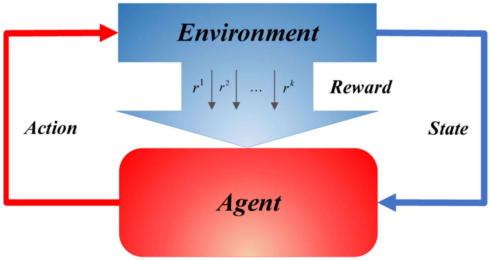
2.1. Reinforcement Learning
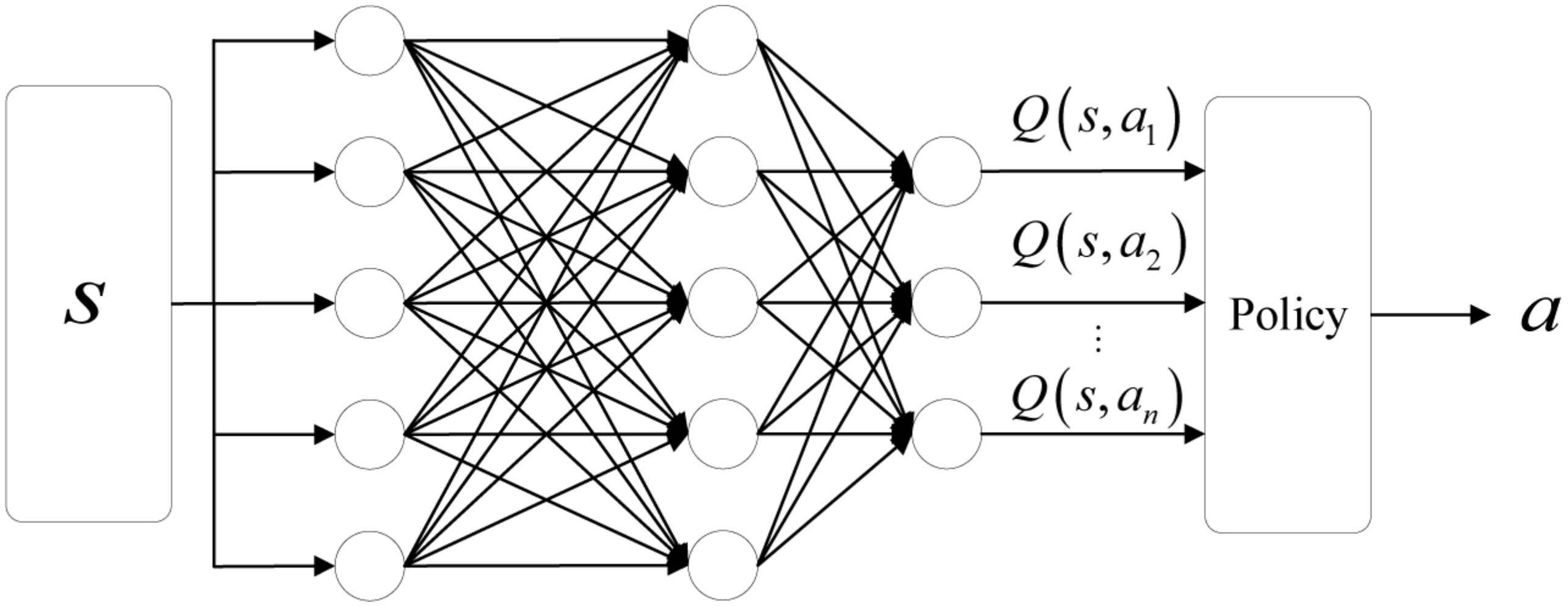
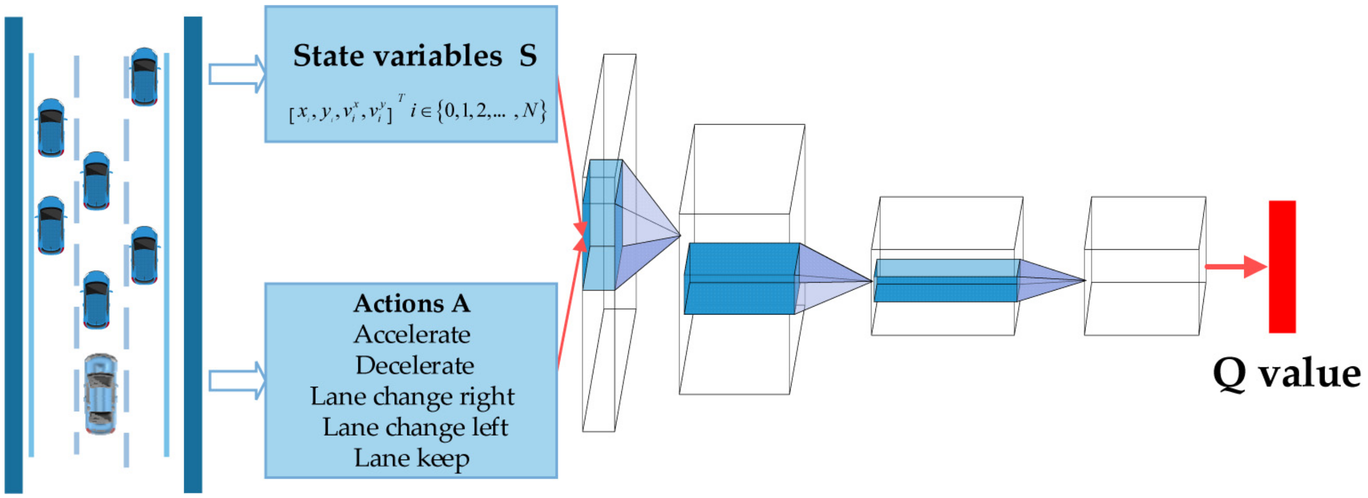
2.2. DQN
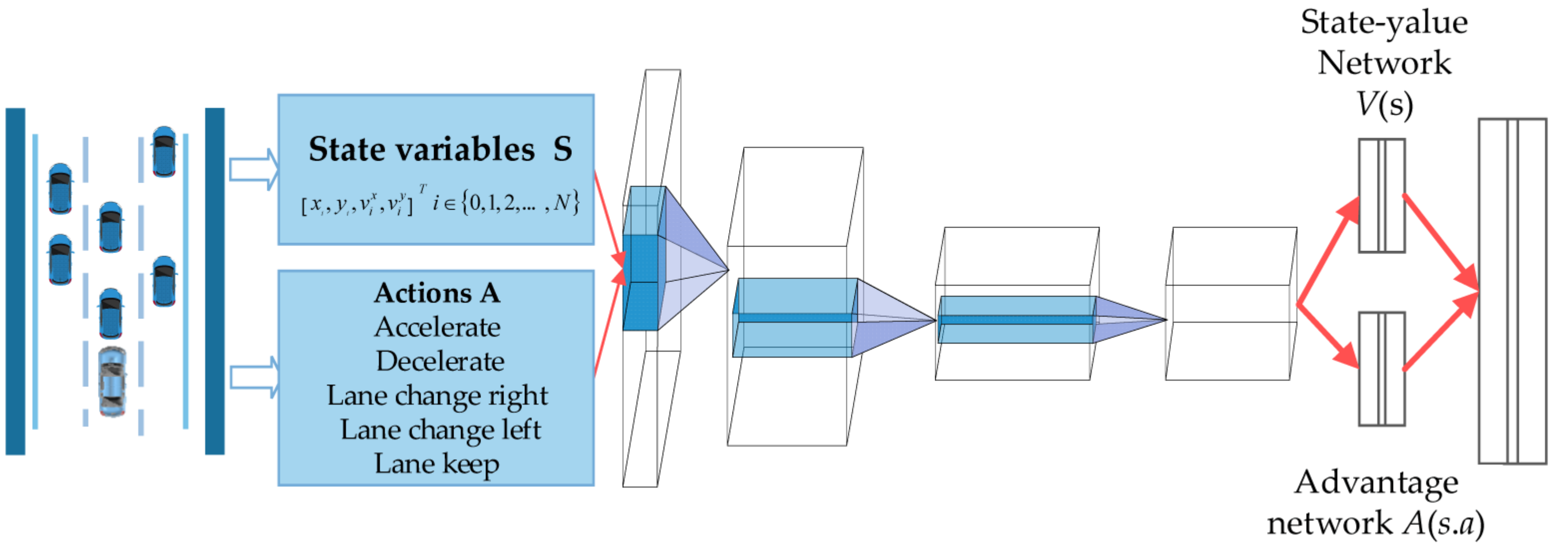
2.3. Dueling DQN
3. Highway Decision-Making Problem
3.1. Problem Formulation
- : Refers to the lateral position of the agent’s center.
- : Refers to the longitudinal position of the agent ’s center.
- : Refers to the lateral velocity of the agent.
- : Refers to the longitudinal velocity of the agent.
- (1)
- Speed Differential: The current speed needs to be lower than the target speed .
- (2)
- Adjacent Lane Speed: The average speed of the vehicles in adjacent lanes should be at least 10 units higher than the current speed () of the ego vehicle.
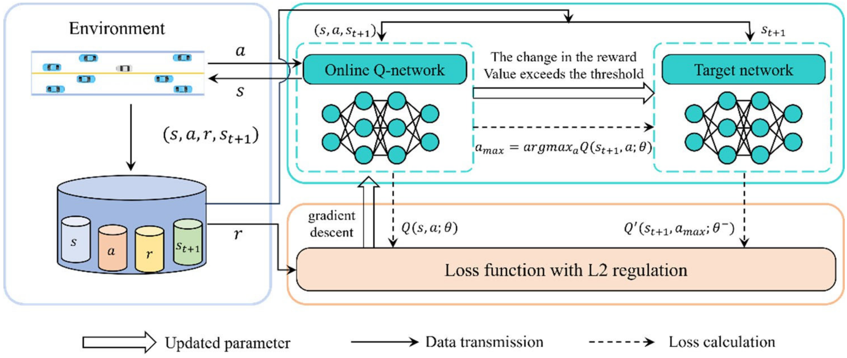
3.2. Huber-Regularized Reward-Threshold Adaptive DDQN
| Algorithm 1 A reward difference triggered target network update strategy |
| Initialize: Online Q-network ,target Q-network with random weights, reward difference threshold K, discount factor , current reward , previous reward . (the value is set to be none) for episode = 1,2…, M do for time step t = 1,2…, T do with a probability of , a random action is chosen; otherwise, the action is selected. current reward If is not none then reward difference = If reward difference > K parameters else no update to target network parameters else previous reward end for end for |
| Algorithm 2 HRA-DDQN |
| Inputs: Replay memory D with capacity N, two Q-networks (online and target). learning rate , discount factor , regularization coefficient , Huber loss threshold ,reward difference threshold K. Initialize: Online Q-network , target Q-network with random weights, replay memory D. for episode = 1,2…, M do for time step t = 1,2…, T do With a probability of , a random action is chosen; otherwise, the action is selected. Execute action , observe reward and the next state . Preprocess the next state and store the transition into the replay memory D. Draw a random minibatch of transitions from D. If is terminal then Set . else Set Perform gradient descent on . If > K then parameters end for end for |
4. Case Studies
4.1. Experimental Setup
4.1.1. Simulator
4.1.2. Parameter Setting
4.1.3. Evaluation Metric
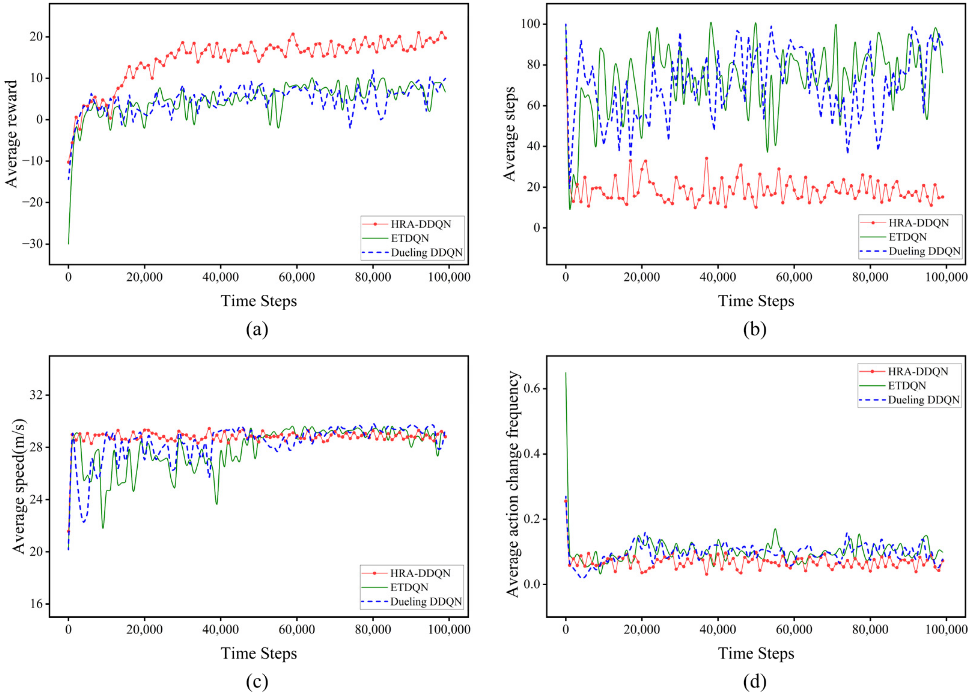
4.2. Case 1: Comprehensive Performance Comparison
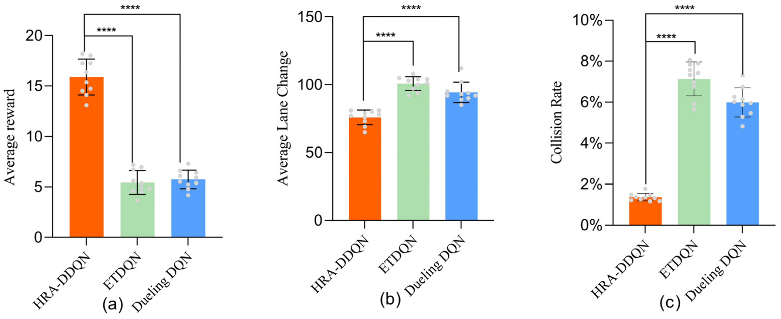
4.2.1. Key Metrics
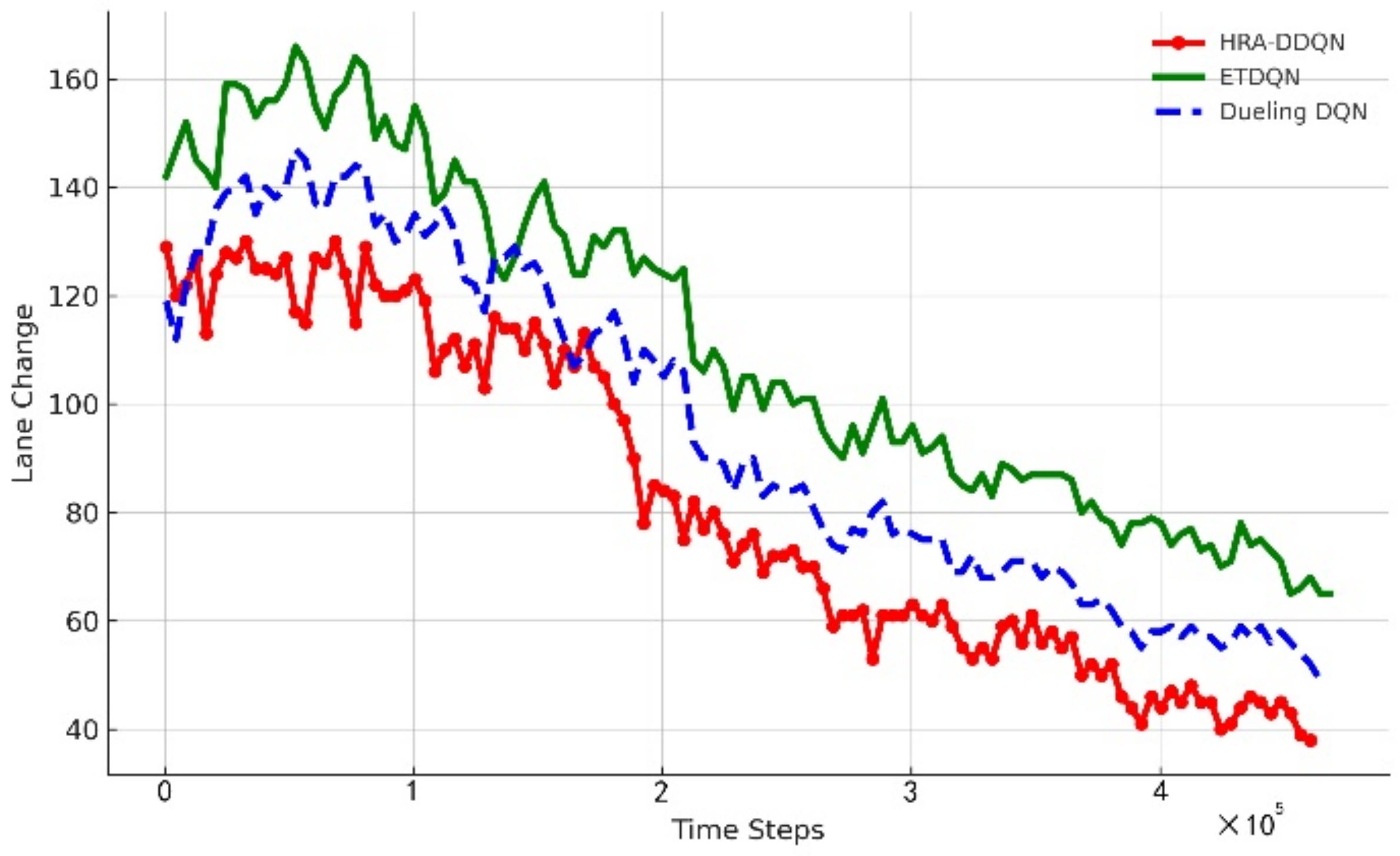
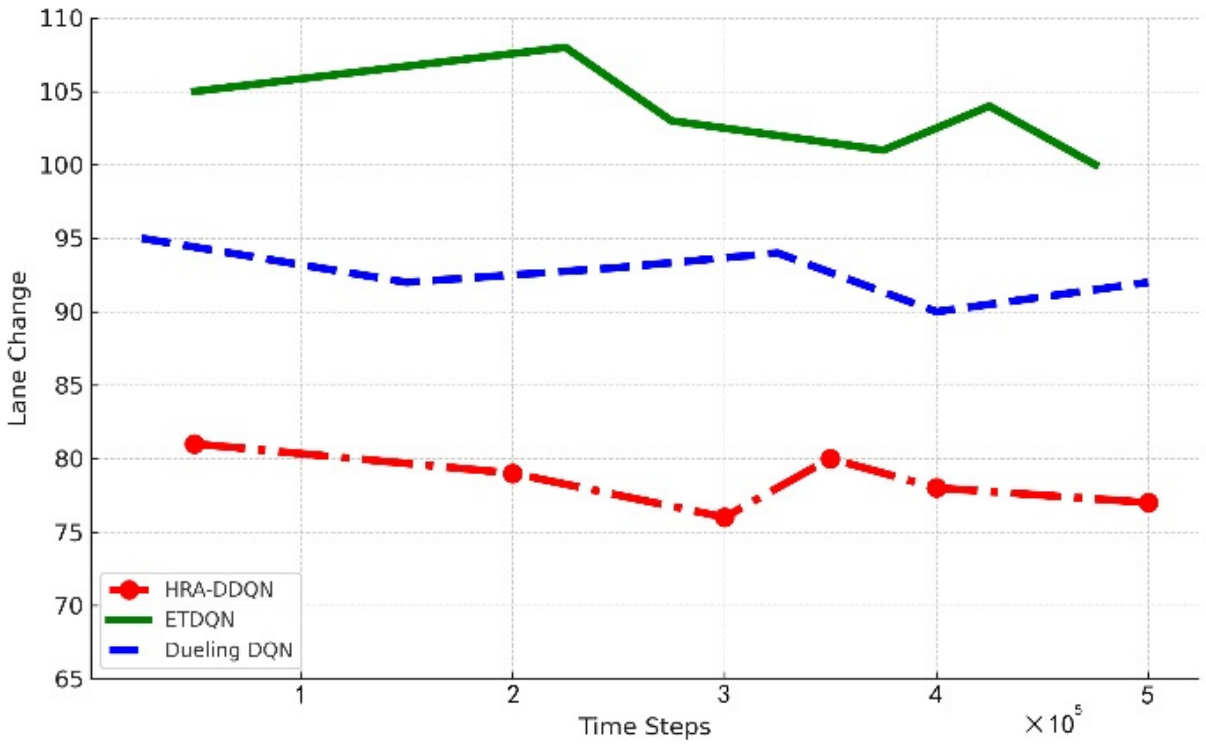
4.2.2. Number of Lane Changes
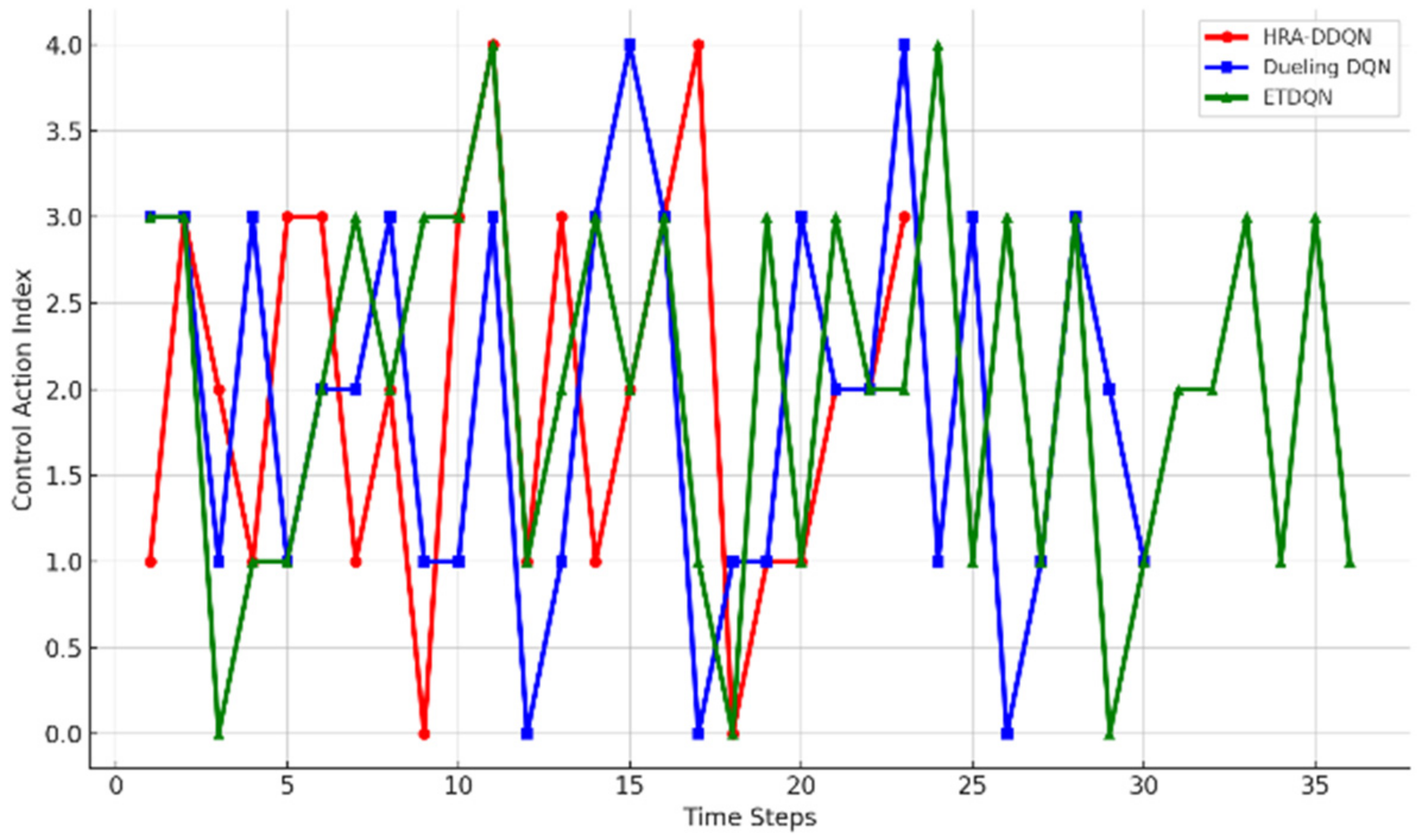
4.2.3. Control Actions
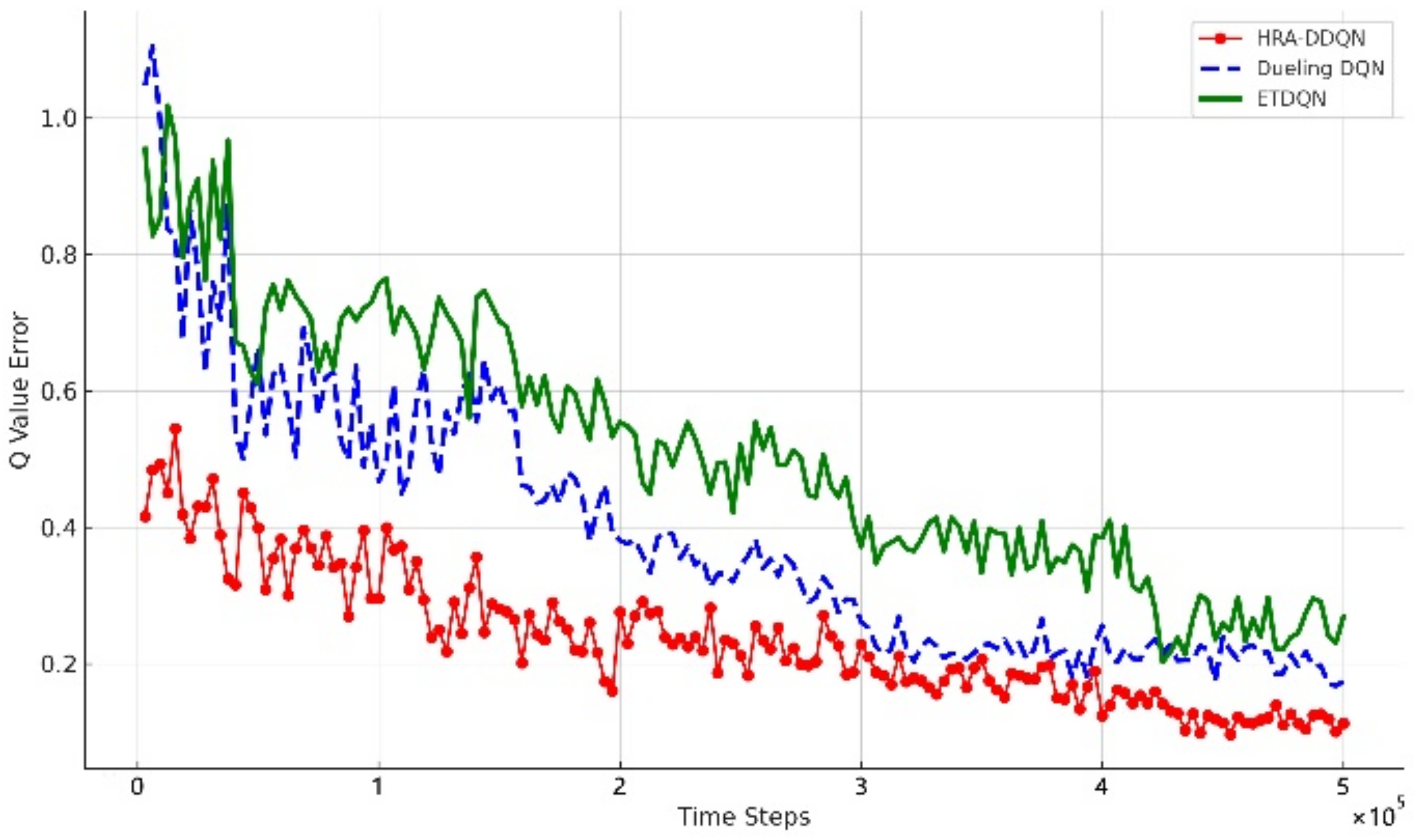
4.2.4. Q-Value Errors
4.2.5. Statistical Analysis
4.2.6. Ablation Study
4.3. Case 2: Ego Vehicle Lane Change Process and Safety Analysis
- (1)
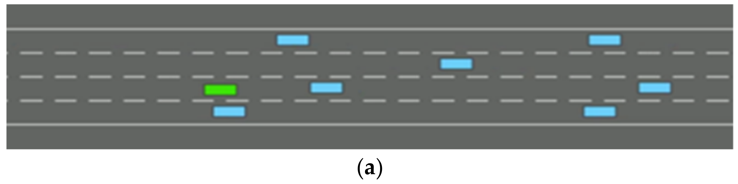
- Lane Change Process and Simulation
- (2)
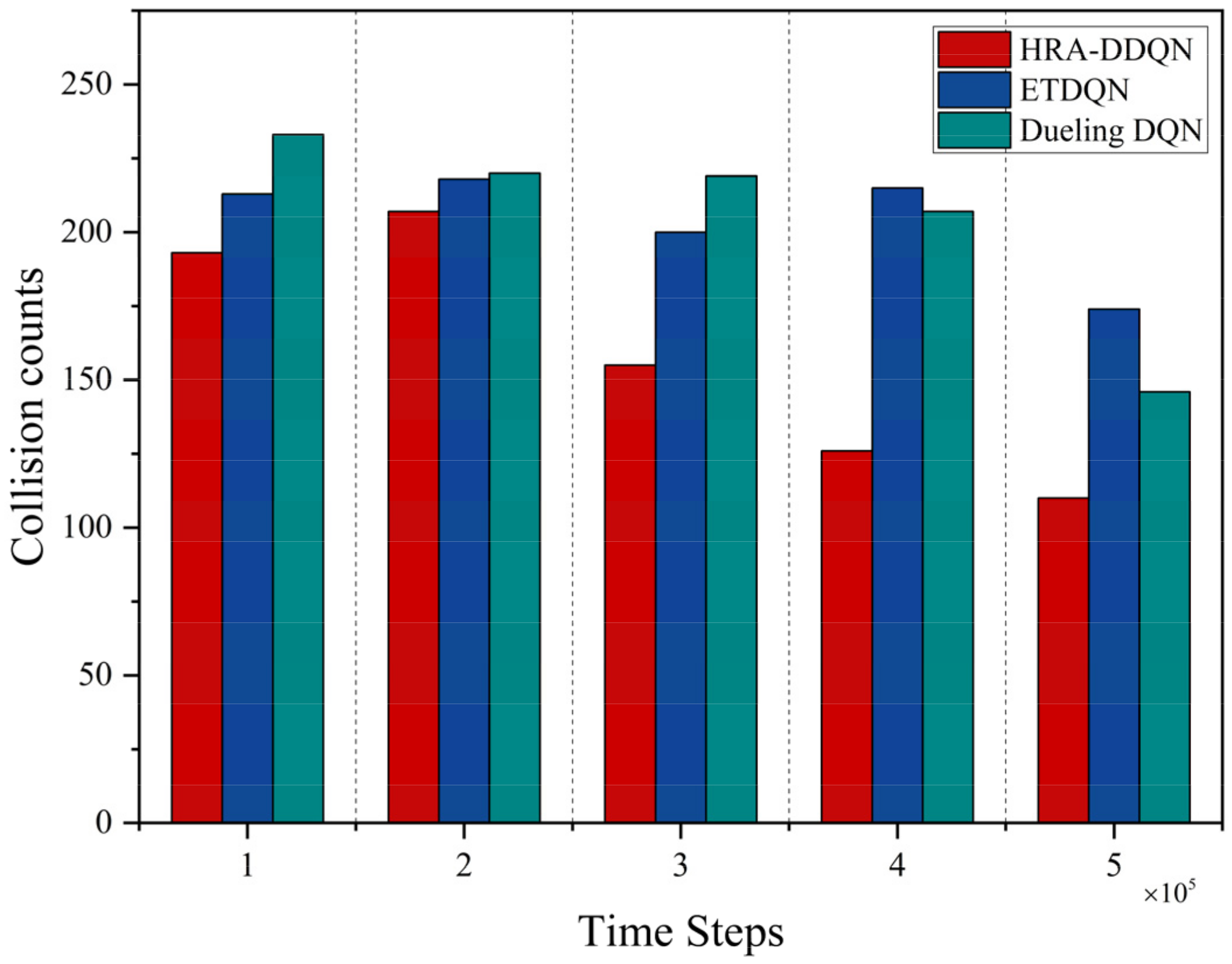
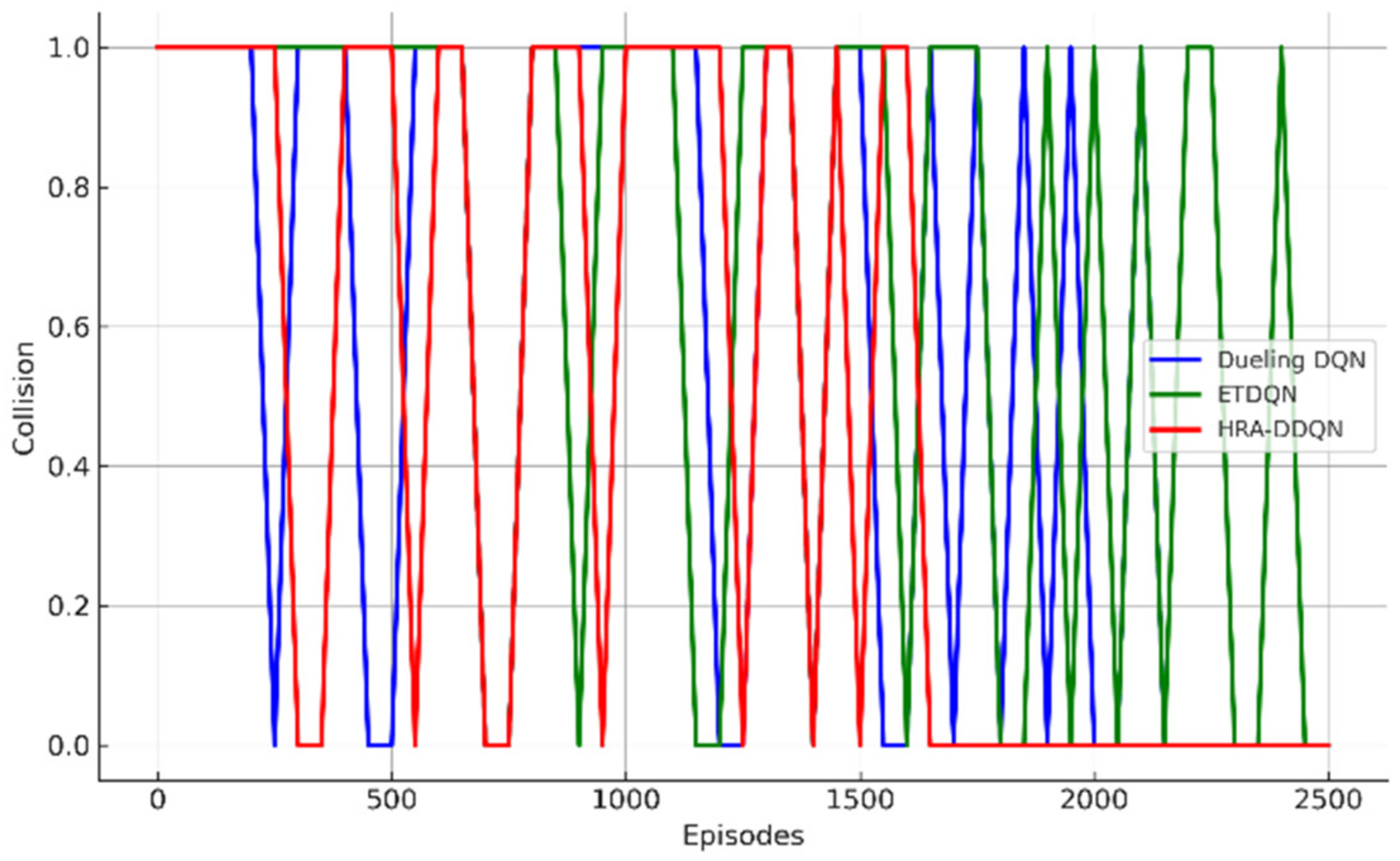
- Safety Evaluation
- (3)
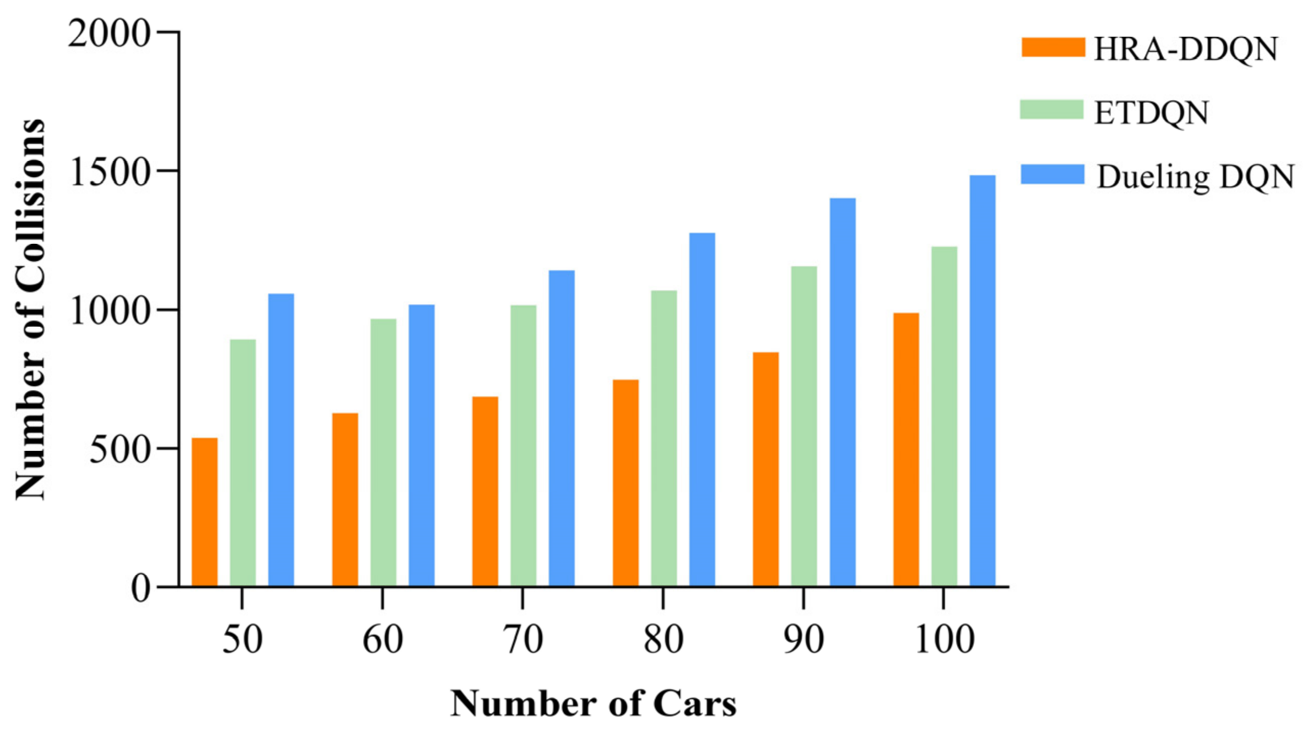
- Collision performance at different vehicle densities
4.4. Case 3: Impact of Key Innovations on Collision Avoidance
5. Conclusions
Author Contributions
Funding
Data Availability Statement
Conflicts of Interest
References
- Feng, S.; Xi, J.; Gong, C.; Gong, J.; Hu, S.; Ma, Y. A collaborative decision making approach for multi-unmanned combat vehicles based on the behaviour tree. In Proceedings of the 3rd International Conference on Unmanned Systems (ICUS), Harbin, China, 27–28 November 2020; pp. 395–400. [Google Scholar]
- Lee, H.; Kim, N.; Cha, S.W. Model-based reinforcement learning for eco-driving control of electric vehicles. IEEE Access 2020, 8, 202886–202896. [Google Scholar] [CrossRef]
- Tian, Y.; Cao, X.; Huang, K.; Fei, C.; Zheng, Z.; Ji, X. Learning to drive like human beings: A method based on deep reinforcement learning. IEEE Trans. Intell. Transp. Syst. 2022, 23, 6357–6367. [Google Scholar] [CrossRef]
- Kiran, B.R.; Sobh, I.; Talpaert, V.; Mannion, P.; Sallab, A.A.A.; Yogamani, S.; Pérez, P. Deep reinforcement learning for autonomous driving: A survey. IEEE Trans. Intell. Transp. Syst. 2022, 23, 4909–4926. [Google Scholar] [CrossRef]
- Chen, J.; Li, S.E.; Tomizuka, M. Interpretable end-to-end urban autonomous driving with latent deep reinforcement learning. IEEE Trans. Intell. Transp. Syst. 2022, 23, 5068–5078. [Google Scholar] [CrossRef]
- Liu, J.; Zhao, L.; Zheng, K.; Zhou, Q. A distributed driving decision scheme based on reinforcement learning for autonomous driving vehicles. In Proceedings of the 91st Vehicular Technology Conference (VTC2020-Spring), Antwerp, Belgium, 25–28 May 2020; pp. 1–5. [Google Scholar]
- Tang, J.; Shaoshan, L.; Pei, S.; Zuckerman, S.; Chen, L.; Shi, W.; Gaudiot, J.-L. Teaching autonomous driving using a modular and integrated approach. In Proceedings of the IEEE 42nd Annual Computer Software and Applications Conference (COMPSAC), Tokyo, Japan, 23–27 July 2018. [Google Scholar]
- Hoel, C.-J.; Driggs-Campbell, K.; Wolff, K.; Laine, L.; Kochenderfer, M.J. Combining planning and deep reinforcement learning in tactical decision making for autonomous driving. IEEE Trans. Intell. Veh. 2020, 5, 294–305. [Google Scholar] [CrossRef]
- Hao, R.; Fan, S.; Dai, Y.; Zhang, Z.; Li, C.; Wang, Y.; Yu, H.; Yang, W.; Yuan, J.; Nie, Z. Rcooper: A real-world large-scale dataset for roadside cooperative perception. In Proceedings of the IEEE/CVF Conference on Computer Vision and Pattern Recognition, Seattle, WA, USA, 16–22 June 2024; pp. 22347–22357. [Google Scholar]
- Liao, J.; Liu, T.; Tang, X.; Mu, X.; Huang, B.; Cao, D. Decision-making strategy on highway for autonomous vehicles using deep reinforcement learning. IEEE Access 2020, 8, 177804–177814. [Google Scholar] [CrossRef]
- Park, M.; Lee, S.Y.; Hong, J.S.; Kwon, N.K. Deep deterministic policy gradient-based autonomous driving for mobile robots in sparse reward environments. Sensors 2022, 22, 9574. [Google Scholar] [CrossRef]
- Wang, L.; Yang, S.; Yuan, K.; Huang, Y.; Chen, H. A combined reinforcement learning and model predictive control for car-following maneuver of autonomous vehicles. Chin. J. Mech. Eng. 2023, 36, 80. [Google Scholar] [CrossRef]
- Do, Q.H.; Tehrani, H.; Mita, S.; Egawa, M.; Muto, K.; Yoneda, K. Human drivers based active-passive model for automated lane change. IEEE Intell. Transp. Syst. Mag. 2017, 9, 42–56. [Google Scholar] [CrossRef]
- Xiong, G.; Kang, Z.; Li, H.; Song, W.; Jin, Y.; Gong, J. Decision–making of lane change behavior based on RCS for automated vehicles in the real environment. In Proceedings of the IEEE Intelligent Vehicles Symposium (IV), Changshu, China, 26–30 June 2018; pp. 1400–1405. [Google Scholar]
- Shu, K.; Yu, H.; Chen, X.; Chen, L.; Wang, Q.; Li, L.; Cao, D. Autonomous driving at intersections: A critical-turning-point approach for left turns. In Proceedings of the IEEE 23rd International Conference on Intelligent Transportation Systems (ITSC), Rhodes, Greece, 20–23 September 2020; pp. 1–6. [Google Scholar]
- Liu, T.; Tian, B.; Ai, Y.; Chen, L.; Liu, F.; Cao, D.; Bian, N.; Wang, F.-Y. Dynamic states prediction in autonomous vehicles: Comparison of three different methods. In Proceedings of the IEEE Intelligent Transportation Systems Conference (ITSC), Auckland, New Zealand, 27–30 October 2019; pp. 3750–3755. [Google Scholar]
- Wei, J.; Dolan, J.M.; Litkouhi, B. A prediction- and cost function-based algorithm for robust autonomous freeway driving. In Proceedings of the IEEE Intelligent Vehicles Symposium, San Diego, CA, USA, 21–24 June 2010; pp. 512–517. [Google Scholar]
- Sethi, S.P.; Zhang, Q. Hierarchical Decision Making in Stochastic Manufacturing Systems; Springer: Berlin/Heidelberg, Germany, 2012. [Google Scholar]
- Paden, B.; Cap, M.; Yong, S.Z.; Yershov, D.; Frazzoli, E. A survey of motion planning and control techniques for self-driving urban vehicles. IEEE Trans. Intell. Veh. 2016, 1, 33–55. [Google Scholar] [CrossRef]
- Siboo, S.; Bhattacharyya, A.; Raj, R.N.; Ashwin, S.H. An empirical study of DDPG and PPO-based reinforcement learning algorithms for autonomous driving. IEEE Access 2023, 11, 125094–125108. [Google Scholar] [CrossRef]
- Schwarting, W.; Alonso-Mora, J.; Rus, D. Planning and decision-making for autonomous vehicles. Annu. Rev. Control Robot. Auton. Syst. 2018, 1, 187–210. [Google Scholar] [CrossRef]
- Chen, Y.; Li, S.; Tang, X.; Yang, K.; Cao, D.; Lin, X. Interaction-aware decision making for autonomous vehicles. IEEE Trans. Transp. Electrif. 2023, 9, 4704–4715. [Google Scholar] [CrossRef]
- Lopez, V.G.; Lewis, F.L.; Liu, M.; Wan, Y.; Nageshrao, S.; Filev, D. Game-theoretic lane-changing decision making and payoff learning for autonomous vehicles. IEEE Trans. Veh. Technol. 2022, 71, 3609–3620. [Google Scholar] [CrossRef]
- Kendall, A.; Hawke, J.; Janz, D.; Mazur, P.; Reda, D.; Allen, J.-M. Learning to drive in a day. In Proceedings of the 2019 International Conference on Robotics and Automation (ICRA), Montreal, QC, Canada, 20–24 May 2019; pp. 8248–8254. [Google Scholar]
- Zhang, S.; Peng, H.; Nageshrao, S.; Tseng, E. Discretionary lane change decision making using reinforcement learning with model-based exploration. In Proceedings of the 2019 18th IEEE International Conference on Machine Learning and Applications (ICMLA), Boca Raton, FL, USA, 16–19 December 2019. [Google Scholar]
- Baheri, A.; Nageshrao, S.; Tseng, H.E.; Kolmanovsky, I.; Girard, A.; Filev, D. Deep reinforcement learning with enhanced safety for autonomous highway driving. In Proceedings of the 2020 IEEE Intelligent Vehicles Symposium (IV), Las Vegas, NV, USA, 19 October–13 November 2020; pp. 1550–1555. [Google Scholar]
- Makantasis, K.; Kontorinaki, M.; Nikolos, I. Deep reinforcement-learning-based driving policy for autonomous road vehicles. IET Intell. Transp. Syst. 2020, 14, 13–24. [Google Scholar] [CrossRef]
- Mnih, V. Playing atari with deep reinforcement learning. arXiv 2013, arXiv:1312.5602. [Google Scholar]
- Al-Hamadani, M.N.A.; Fadhel, M.A.; Alzubaidi, L.; Balazs, H. Reinforcement Learning Algorithms and Applications in Healthcare and Robotics: A Comprehensive and Systematic Review. Sensors 2024, 24, 2461. [Google Scholar] [CrossRef]
- Bergerot, C.; Barfuss, W.; Romanczuk, P. Moderate confirmation bias enhances decision-making in groups of reinforcement-learning agents. PLoS Comput. Biol. 2024, 20, e1012404. [Google Scholar] [CrossRef]
- Van Hasselt, H.; Guez, A.; Silver, D. Deep reinforcement learning with double q-learning. In Proceedings of the AAAI Conference on Artificial Intelligence, Phoenix, AZ, USA, 12–17 February 2016; Volume 30. [Google Scholar] [CrossRef]
- Iqbal, A.; Tham, M.L.; Chang, Y.C. Double deep Q-network-based energy-efficient resource allocation in cloud radio access network. IEEE Access 2021, 9, 20440–20449. [Google Scholar] [CrossRef]
- Huang, L.; Ye, M.; Xue, X.; Wang, Y.; Qiu, H.; Deng, X. Intelligent routing method based on Dueling DQN reinforcement learning and network traffic state prediction in SDN. Wireless Netw. 2024, 30, 4507–4525. [Google Scholar] [CrossRef]
- Din, N.M.U.; Assad, A.; Sabha, S.U.; Rasool, M. Optimizing deep reinforcement learning in data-scarce domains: A cross-domain evaluation of double DQN and dueling DQN. Int. J. Syst. Assur. Eng. Manag. 2024. [Google Scholar] [CrossRef]
- Guan, Y.; Li, S.E.; Duan, J.; Wang, W.; Cheng, B. Markov probabilistic decision making of self-driving cars in highway with random traffic flow: A simulation study. J. Intell. Connect. Veh. 2018, 1, 77–84. [Google Scholar] [CrossRef]
- He, X.; Yang, H.; Hu, Z.; Lv, C. Robust lane change decision making for autonomous vehicles: An observation adversarial reinforcement learning approach. IEEE Trans. Intell. Veh. 2022, 8, 184–193. [Google Scholar] [CrossRef]
- Sharma, O.; Sahoo, N.C.; Puhan, N.B. Highway lane-changing prediction using a hierarchical software architecture based on support vector machine and continuous hidden markov model. Int. J. Intell. Transp. Syst. Res. 2022, 20, 519–539. [Google Scholar] [CrossRef]
- Zhu, Z.; Zhao, H. A survey of deep RL and IL for autonomous driving policy learning. IEEE Trans. Intell. Transp. Syst. 2021, 23, 14043–14065. [Google Scholar] [CrossRef]
- Chae, H.; Kang, C.M.; Kim, B.D.; Kim, J.; Chung, C.C.; Choi, J.W. Autonomous braking system via deep reinforcement learning. In Proceedings of the 2017 IEEE 20th International Conference on Intelligent Transportation Systems (ITSC), Yokohama, Japan, 16–19 October 2017; pp. 1–6. [Google Scholar]
- Xia, W.; Li, H.; Li, B. A control strategy of autonomous vehicles based on deep reinforcement learning. In Proceedings of the 2016 9th International Symposium on Computational Intelligence and Design (ISCID), Hangzhou, China, 10–11 December 2016; Volume 2, pp. 198–201. [Google Scholar]
- Li, G.; Yang, Y.; Li, S.; Qu, X.; Lyu, N.; Li, S.E. Decision making of autonomous vehicles in lane change scenarios: Deep reinforcement learning approaches with risk awareness. Transp. Res. Part C Emerg. Technol. 2022, 134, 103452. [Google Scholar] [CrossRef]
- Sharma, S.; Tewolde, G.; Kwon, J. Lateral and longitudinal motion control of autonomous vehicles using deep learning. In Proceedings of the 2019 IEEE International Conference on Electro Information Technology (EIT), Brookings, SD, USA, 20–22 May 2019; pp. 1–5. [Google Scholar]
- Kim, K. Enhancing Reinforcement Learning Performance in Delayed Reward System Using DQN and Heuristics. IEEE Access 2022, 10, 50641–50650. [Google Scholar] [CrossRef]
- Leurent, E. An Environment for Autonomous Driving Decision-Making. Available online: https://github.com/Farama-Foundation/HighwayEnv (accessed on 26 September 2024).
- Lu, J.; Han, L.; Wei, Q.; Wang, X.; Dai, X.; Wang, F.-Y. Event-triggered deep reinforcement learning using parallel control: A case study in autonomous driving. IEEE Trans. Intell. Veh. 2023, 8, 2821–2831. [Google Scholar] [CrossRef]


| Hyperparameters | Symbol | Value |
|---|---|---|
| Discount factor | γ | 0.97 |
| Learning rate | h | 0.1 |
| Batch size | B | 256 |
| Replay buffer size | N | 8192 |
| Speed reward weight | cv | 0.5 |
| Collision reward weight | Cc | 5 |
| Lane-keeping reward weight | cl | 0.1 |
| Lane-changing reward weight | cd | 0.5 |
| Action stability reward weight | ce | 2 |
| Evaluation Metric | HRA-DDQN | ETDQN | Dueling DQN |
|---|---|---|---|
| Average reward | 14.5308 | 4.5162 | 4.7969 |
| Average speed | 29.8305 | 27.8895 | 28.3431 |
| Average number of steps | 19.05 | 73.302 | 70.63 |
| Average action change frequency | 6.938% | 10.27% | 9.71% |
| Collision rate | 1.37% | 7.33% | 5.95% |
| cv | cc | cl | cd | ce | |
|---|---|---|---|---|---|
| Base group | 0.5 | 5 | 0.1 | 0.5 | 2 |
| Experiment 1 | 1 | 5 | 0.1 | 0.5 | 2 |
| Experiment 2 | 0.5 | 2 | 0.1 | 0.5 | 2 |
| Experiment 3 | 0.5 | 5 | 0.5 | 0.5 | 2 |
| Average Reward | Average Speed | Collision Rate | Average Lane Change | |
|---|---|---|---|---|
| Base group | 15.68 | 29.81 | 1.29% | 79 |
| Experiment 1 | 11.54 | 30.14 | 3.13% | 91 |
| Experiment 2 | 9.64 | 28.47 | 5.41% | 85 |
| Experiment 3 | 14.62 | 29.37 | 1.78% | 75 |
| Experiment 4 | 10.46 | 28.85 | 1.81% | 82 |
| Experiment 5 | 12.28 | 29.17 | 2.36% | 84 |
| Collision Rate | Average Number of Lane Changes | Average Q-Value Error | |
|---|---|---|---|
| HRA-DDON | 1.16% | 82 | 0.217 |
| Method 1 | 2.27% | 107 | 0.389 |
| Method 2 | 2.83% | 92 | 0.542 |
| Method 3 | 3.84% | 119 | 0.309 |
| K | Collision Rate | Average Lane Change | Average Reward |
|---|---|---|---|
| 0.1 | 7.31% | 121 | 4.55 |
| 0.25 | 2.59% | 97 | 11.31 |
| 0.5 | 1.37% | 84 | 14.64 |
| 0.8 | 3.94% | 72 | 9.47 |
| 1 | 5.56% | 65 | 5.13 |
Disclaimer/Publisher’s Note: The statements, opinions and data contained in all publications are solely those of the individual author(s) and contributor(s) and not of MDPI and/or the editor(s). MDPI and/or the editor(s) disclaim responsibility for any injury to people or property resulting from any ideas, methods, instructions or products referred to in the content. |
© 2025 by the authors. Licensee MDPI, Basel, Switzerland. This article is an open access article distributed under the terms and conditions of the Creative Commons Attribution (CC BY) license (https://creativecommons.org/licenses/by/4.0/).
Share and Cite
Wang, Z.; Jiang, M.; Gu, S.; Gu, Y.; Wang, J. Enhancing Lane Change Safety and Efficiency in Autonomous Driving Through Improved Reinforcement Learning for Highway Decision-Making. Electronics 2025, 14, 918. https://doi.org/10.3390/electronics14050918
Wang Z, Jiang M, Gu S, Gu Y, Wang J. Enhancing Lane Change Safety and Efficiency in Autonomous Driving Through Improved Reinforcement Learning for Highway Decision-Making. Electronics. 2025; 14(5):918. https://doi.org/10.3390/electronics14050918
Chicago/Turabian StyleWang, Zi, Mingzuo Jiang, Shaoqiang Gu, Yunyang Gu, and Jiaxia Wang. 2025. "Enhancing Lane Change Safety and Efficiency in Autonomous Driving Through Improved Reinforcement Learning for Highway Decision-Making" Electronics 14, no. 5: 918. https://doi.org/10.3390/electronics14050918
APA StyleWang, Z., Jiang, M., Gu, S., Gu, Y., & Wang, J. (2025). Enhancing Lane Change Safety and Efficiency in Autonomous Driving Through Improved Reinforcement Learning for Highway Decision-Making. Electronics, 14(5), 918. https://doi.org/10.3390/electronics14050918