Abstract
This paper focuses on a solution of target self-positioning when a Global Navigation Satellite System (GNSS) is denied. It is composed of Inertial Navigation Systems (INS), Signals of Opportunities (SOPs), and a navigation prototype. One of the options for navigation via SOP (NAVSOP) is to utilize cellular signals, such as Long Time Evolution (LTE). When the prior information is insufficient, the location of the base station (BS) is obtained by collecting the demodulation of the downlink signal, and the synchronization signal is used for static time offset correction. In view of the large positioning error of the trilateral positioning method based on Received Signal Strength (RSS), a multi-station positioning optimization method is proposed by introducing the robust regression. Monte Carlo simulation experiments indicate that the method has improved the positioning failure and insufficient accuracy. Aiming at the influence of the state estimation errors on filtering results, the Second Order Mutual Difference (SOMD) method with the noise covariance R, which is independent of the existing Extended Kalman Filter (EKF) framework and combined with Redundant Measurement Noise Covariance Estimation (RMNCE), is applied to the model. The simulation results show that the average error of the robust model is 10.28 m, which is better than the EKF method. Finally, a vehicle test in constant speed has been carried out. The results show that the proposed model can realize self-positioning with limited BS location information, and the positioning accuracy can reach 11.68 m over a 283 m trajectory.
1. Introduction
With the popularity and performance improvement of intelligent devices, target self-positioning has attracted more scholars to conduct related research [1,2,3]. In view of the diversity and complexity of the environment, the existing navigation relying on INS and GNSS will be difficult to ensure high performance, high availability, and high reliability [4]. Wireless sensor networks composed of SOP are an important edge technology in navigation and positioning [5]. Figure 1 indicates that SOP-assisted INS can be used when the GNSS is cut-off.
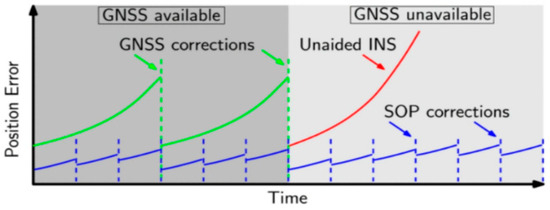
Figure 1.
NAVSOP application scenario.
LTE is a strict synchronization communication system in both the time and frequency domains that has been commercially mature anywhere in China, which can be used for positioning. As shown in Figure 2, ubiquitous, small, low-cost devices are becoming more and more popular, and opportunistic emission sources such as cellular base stations can be used to augment, complement, and back-up satellite navigation. The coverage of each BS is usually overlapped when the macro-station is distributed. The target may detect multiple transmitted signals at the same time, and the Received Signal Strength (RSS) information is introduced into the wireless sensor network and converted into the distance value of each macro-station to the receiver. It is an effective positioning strategy [6].
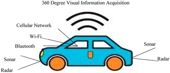
Figure 2.
Vehicle-mounted NAVSOP.
The concept of robust linear regression aims at finding the parameters of linear equation from noise data with abnormal values and is widely used in data analysis, navigation, and positioning. Reference [7] introduces a robust regression algorithm and designs an iterative outlier removal algorithm based on correlation; the experiment results show that the outliers can be effectively removed in a normal-distributed or uniform-distributed dataset. Reference [8] considers the use of deep neural networks in the context of robust regression, builds upon Huber’s robust regression and the classical least trimmed squares estimator, and proposes a deep neural network that generalizes both and provides high accuracy with low computational complexity.
As the positioning is completed, it is necessary to smooth and filter the pseudo-measurement, get a track closer to the real state, reduce the positioning error, and predict state at the next moment. Aiming at the problem that most filtering algorithms cannot guarantee the objective acquisition of noise statistical characteristics, reference [9] introduces an enhanced adaptively of unscented particle filter architecture exploits an adaptive logic composed by a pre-processing stage and a run-time error covariance estimation to improve navigation accuracy and estimation robustness. Reference [10] proposes an algorithm for estimating the observation noise variance with SOMD sequence based on redundant measurement. The main idea is to calculate the first-order self-difference sequence of the two sequences, respectively, according to the change relationship of the measurement sequences when there are two different observation systems for the observed object SOMD sequence, and the statistical characteristics of the noise of the observation system are obtained via statistical methods. Reference [11] introduces an SOMD algorithm into a non-redundant measurement system and constructs the envelope pseudo-measurement noise covariance estimation; by extracting the upper and lower envelope of the signal, the median of each sampling point is calculated to form a pseudo-measurement system. The SOMD algorithm has the following advantages: (1) noise estimation is independent of the filtering system and realizes the decoupling of noise estimation and filtering state estimation; (2) the deterministic error of the measurement system is usually stable in a short time, which can be eliminated by solving the first-order self-differential sequence; (3) sometimes, the target may have state mutation, the SOMD sequence can completely eliminate it, and then only the random noise term is retained.
The GNSS-assisted INS model based on the EKF couples INS and GNSS in one of the following ways [12]: (1) loose coupling, fusing INS and GNSS position and velocity solutions; (2) tight coupling, fusing INS solutions with GNSS pseudo distance; (3) deep coupling, using INS solutions to help the tracking loop of the GNSS receiver [13]. Tightly coupled systems can be implemented using most commercial off-the-shelf (COTS) components and can still provide EKF assisted updates in scenarios with at least three BS signals, which is not the case in loosely coupled systems [14]. Therefore, this paper attempts to construct a tightly combined SOP/INS navigation model [15].
This article presents several challenges:
- In certain environments with diversity and complexity, the locations of the base stations that the target passes through cannot be predicted, treating the BS locations as estimators leads to the expansion of the state equations, which complicates real-time navigation.
- The basic trilateration algorithm has the problem of location ambiguity, which cannot guarantee the existence and uniqueness of the solution [16]; the least squares multilateral positioning method does not have a weight function affects the results of linear regression, resulting in more outliers that affect the location.
- Currently, most adaptive filtering algorithms cannot ensure the acquisition of noise statistical characteristics based on the choice of computation, and their measurement noise variance heavily depends on the estimated state, measurement true values, and systematic errors in the measurement values.
Considering the above problems, the innovations of this study are as follows:
- For unknown BS location, the calculation module is considered to calculate the information of BS location by LTE demodulation.
- The bi-square weights function of robust regression is introduced into the RSS path loss attenuation model, which verifies that this method can effectively eliminate the maximum deviation measurement and ensure the stability of the positioning solution.
- In scenarios where the statistical characteristics of noise are unknown or without any prior knowledge, the SOMD method is used to adaptively adjust the filtering gain under RMNCE module, and an evaluation criterion is also introduced to eliminate the estimated values with large noise covariance.
This paper mainly discusses the research on the SOP-positioning problem under Radio SLAM mode [12]; that is, the GNSS is unavailable, and the INS is available. In the rest of this paper, we will introduce the recent related work in Section 2. Section 3 presents the related methods: BS location calculation, receiver time offset correction, multilateral positioning optimization, RMNCE. Section 4 proposes a chance signal navigation model combined with INS; by judging measurement outliers based on this model, an enhanced navigation scheme is implemented. Section 5 introduces the experimental part, including experimental method, platform route, and the on-board test result. Section 6 includes a summary and outlook on the research of the paper.
2. Related Work
In passive positioning systems, on the one hand, the arrival time of the signal generated by the terminal movement is extracted by time synchronization with the BS, and on the other hand, the identification information system of the BS is also extracted by using the broadcast characteristics of the Signal Information Block 1 (SIB1). SIB1 information contains MCC, MNC, TAC, CI, and other BS information. Since the MAC address is device-independent and geographically traceable, it can be used as a unique identification of the BS, and the MAC address can be compared with the online or offline database; that is, the BS location measurement can be obtained. According to the information of BS location and INS information, the target track is determined. In the case that the BS position is unknown, if the downlink signal characteristics can be analyzed and the SIB1 information can be extracted, the BS position can be used as an estimator. Figure 3 shows the general downlink demodulation process of LTE, including cell search, time–frequency estimation, PBCH decode (located in the 0th LTE subframe), PCFICH decode, PDCCH decode (located in the 5th LTE subframe), and sampling.
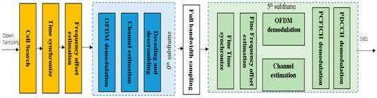
Figure 3.
LTE downlink demodulation.
The instantaneous slant distance between the platform and the radiation source is constantly changing, and the cellular-signal-transmitting end has a clear periodicity, so the received signal frame period is different from that of the radiation-source-transmitting signal frame period; when the slant distance between the platform and the radiation source becomes shorter, the received signal frame period is shortened, the platform and the radiation source slant distance becomes longer and, the received signal frame period increases. The influence of receiver clock error on frame head offset cannot be ignored when solving the radiation source data collected by the receiver.
The key link of RSS location method of BS is to establish an accurate path loss numerical model [17,18,19,20,21,22], reverse the distance from each macro-station to the receiver, and obtain target position by using the trilateration measurement method. Table 1 describes several LTE path attenuation models related to RSS.

Table 1.
Cellular signal strength path attenuation model.
On the backhaul link, infected by the limited conversion accuracy of ADC and other components, as well as the drift of the temperature, noise, mismatch of the antenna, and other factors, RSS accuracy can generally only be accurate to the integer. For Non-Line Of Sight (NLOS) scenarios, reference [23] provides a more comprehensive assessment of path loss by considering factors such as atmospheric gas attenuation, atmospheric scattering attenuation, and building-incident path loss in urban environments.
As the geographical location and RSS information are achieved, the position can be calculated, and the positioning can be realized when the position of the target device to the three radiation sources is reflected as three circles exactly intersecting at one point. In the actual process, due to the diffraction and multipath of electromagnetic waves, multipath, and other problems, the observed value of the RSS may have a large deviation from the actual value assumed by the empirical model, which is reflected as a distance deviation of 100 m, and the situations are shown in Figure 4: (1) pseudo-range pollution leads to the shortening of the observed distance value from the three base stations to the target, there is no intersection between the base station and the distance circle, and the equation is under-solved, which may produce random or approximate values; (2) attenuation factors cause the observed distance values of some base stations to the target to become larger, there are 2~3 intersection points between the circles, and only one random solution can be obtained; (3) there are 3~4 intersections between the circles due to the superposition of interference factors, and only one of the random solutions can be taken, in which case it is most likely to produce a large error. The above-mentioned problems need to be overcome by using RSS to achieve positioning. The trilateral positioning algorithm with the strongest signal is taken as the basic algorithm for auxiliary positioning, and an improved algorithm is gradually proposed.
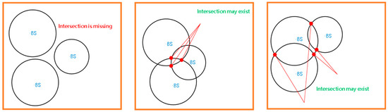
Figure 4.
Failure of trilateral positioning.
As the distance between the target position and the BS increases, the distance observation errors, caused by other interference factors such as measurement error of RSS and multipath, increases, and the probability of positioning failure increases [24]. The traditional EKF measurement noise covariance matrix is unchanged, the accuracy of the predicted value decreases with the loss of lock time when the GNSS is denied, and the measurement noise covariance matrix should change accordingly. At this time, the adaptive Kalman filter (AKF) performs an online estimation of the measurement noise covariance matrix to improve the filtering accuracy. This algorithm cannot guarantee the objective acquisition of the statistical characteristics of noise in the selection of a calculation basis. In most practical applications, the statistical characteristics of noise are usually unknown and are often replaced by empirical values. The adaptive estimation based on multiple models and based on new information or residual [25] couples the estimation error of the state quantity. When the state estimation error is large, it will affect the estimation and adjustment of the noise variance matrix or state error covariance matrix of the system, resulting in inaccurate or even divergent filter output [26]. Therefore, it is necessary to analyze the problem that the filter results are affected by the state estimation error, so as to provide reliable data support for system. In addition, when the pseudo-range jump cannot form a fast identification, it will affect the accuracy of the subsequent filter solution; in view of this, it is necessary to implement the fault detection of the pseudo-range of SOP. The random weighting method is introduced into the measurement covariance estimation to control the accuracy level of outliers, which overcomes the limitation of the RMNAE method and has stronger robustness to the estimation of noise characteristics. By complementing the desired attributes of each technology, a highly robust and accurate navigation solution is achieved in urban environments.
3. Positioning Methods
3.1. BS Location Calculation in LTE Downlink
As shown in Appendix A, the downlink signal at the receiver is parsed to obtain the location information of the LTE BS, which includes the following:
- Timing synchronization: determine the position of the first subframe of the received signal, and identify the cell ID number.
- Cyclic Prefix (CP)-type detection.
- Integer and decimal frequency offset estimation and compensation.
- Channel estimation.
- Decode PBCH, determine the system bandwidth and System Frame Number (SFN), determine whether SIB1 is possible in the current frame, and if so, sample the full bandwidth of the 5th subframe.
- Decode PCFICH to determine the time-frequency position of the PDCCH.
- Extract SIB1 information after blind search for DCI in PDCCH.
3.2. Static Data-Based Clock Biases Correction
3.2.1. Time-Offset Extraction
When extracting the cell ID information for LTE dynamic data, the received 28 MHz signal needs to be resampled to the full bandwidth 30.72 MHz, and the frame synchronization of the full bandwidth resampled signal is performed to determine the position of the frame header. Assuming that the receiver clock is accurate, the change in the slant distance from the platform to the radiant source at each time can be obtained; there are 848 frames of SIB1 data in 17 s received data, which can determine the offset of the frame head as shown in Figure 5. This result is inconsistent with the actual platform moving at 60 km/h towards the radiant source, which further confirms that the clock of the receiver is offset, and the clock offset of the receiver needs to be corrected.
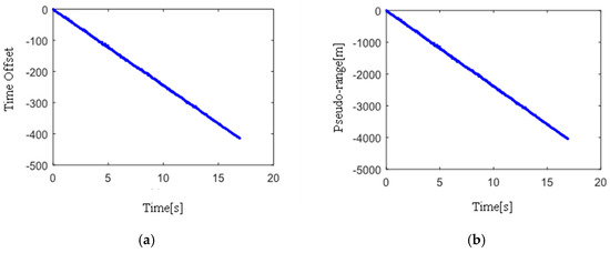
Figure 5.
Received signal clock offset: (a) time-offset extraction; (b) pseudo-range extraction.
3.2.2. Time-Offset Correction
According to the performance indicators in the receiver manual, the internal time base aging rate is 0.5 × 10⁻⁶/year. As the clock offset change is a slow change process, a set of static data can be collected when the platform is stationary, and the clock offset can be estimated by frame head offset. The pseudo-range between the platform and the radiation source does not change when the platform is stationary, and the frame head offset of the static data, including the clock error, is measured as follows:
The change in the static data should be linear, and the clock bias error in dynamic data can be corrected using a point-by-point correction method.
Figure 6 shows the effect of time offset correction. In addition, since the time bias of static data changes linearly, the linear regression method can also be used for consistent correction of dynamic data to reduce the impact of quantization errors.
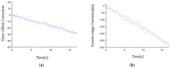
Figure 6.
Correction based on static data: (a) signal frame header offset correction; (b) signal pseudo-distance difference correction.
3.3. Robust Regression-Based Multilateral Positioning
According to the relationship between RSS and the distance, an appropriate path loss numerical model is necessary to invert the distance from LTE macro-station to the receiver. Since the 3rd Generation Partnership Project (3GPP) protocol 36.101 [27] specifies a wide range of LTE frequencies, selecting a model independent of the operating frequency can reduce the influence of input variables on the path loss. As the SOP standards studied in this paper are proposed by the 3GPP organization, a revised 3GPP model proposed in reference [28] is adopted. The analysis shows that the RSS prediction accuracy is less than 0.37 dB, which shows good agreement with measurements. The expression is as follows:
where is expressed as follows:
is the antenna height of the relay station in meter, and is the distance between the base station and the relay station in meter, .
When the three anchor points and the distance from the target to the anchor point are known, the height information is not considered in the two-dimensional plane, and the three-circle intersection point is the position of the unknown point. Assuming that the actual position of the reference point is obtained by the INS, the positioning error at moment t is defined as follows:
Then, the estimated Root Mean Square Error (RMSE) value for each location is calculated, defined as follows [29]:
As shown in Appendix B, the trilateral positioning algorithm selects BS with the three largest RSS at the current moment to perform location estimation; its complexity is low, the positioning speed is fast, and the abnormal situation shown in Figure 4 may occur in the positioning process. In fact, the situation assumed by the algorithm is ideal, and its positioning solution is unstable, and the existence and uniqueness of the solution cannot be guaranteed [16]. In some network environments, more than 10 BSs signals can often be detected at a certain location; thus, the information set used is narrow. Now the positioning equation is reconsidered, and the positioning method based on least square optimization is used to improve the positioning accuracy. The least square method is a method to find the best regression function by minimizing the sum of squares of absolute error. It is essentially unbiased estimation and has no weight function. Therefore, the existence of the maximum deviation measurement has a significant impact on the regression results, resulting in more outliers affecting the positioning results in the aforementioned linear regression process.
In order to improve this problem, the concept of robust regression is introduced, which can fit most data structures and identify potential outliers or structures that deviate from the model assumptions. Iterative reweighting least squares based on the bi-square weights function uses least squares to find a curve that fits most of the data and is generally preferred over least absolute residuals, while minimizing the impact of outliers [30]. In this paper, the bi-square weights model is used. Theoretically, the estimate is almost consistent with the least square estimate when the error is normally distributed, and the result is superior to the least absolute residuals estimate when the error term is not subject to normal distribution [31].
In a 500 m × 500 m area, 20 BSs are randomly generated, and the pseudo-range is calculated by using the path attenuation model in reference [28] and the RSS indicator with a RMSE of 0.1 dB. Figure 7 shows the positioning errors and error probability distribution of 250 Monte Carlo simulations of the above algorithms. From Figure 7a, in the low-error zone with an error less than 20 m, the error performance of robust linear regression was similar to that of trilateral positioning; however, in the region where the error was greater than 40 m, the probability of robust linear regression producing large error is significantly lower than that of trilateral positioning. The probability of the former positioning error greater than 40 m was not higher than 4%, while the latter was about 10%. From Figure 7b, the trilateral and ordinary least squares method had errors greater than 100 m; the former also had a small number of large errors; robust linear regression rarely had an error greater than 40 m. Robust regression was significantly superior to the other two algorithms in positioning accuracy and error probability, and there was no failure occurred in the positioning simulation.
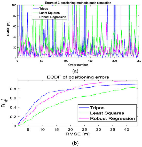
Figure 7.
Comparison of simulation effects of three positioning methods: (a) positioning-error analysis; (b) positioning-error probability distribution.
Seen from Table 2, the RMSE of robust regression was 13.7 m, which was superior to the other two algorithms. This was due to the fact that when the minimum error was close, the outliers of the maximum errors of the trilateral positioning and the least squares method were greater than 100 m. When the deviation of the outlier was large, the regression results were interfered with. The above results further demonstrated the superiority of robust regression in improving the mutation points.
Table 2.
Positioning error of multilateral positioning algorithm.
3.4. Redundant Measurement Noise Estimation Filtering
3.4.1. SOMD Noise Estimation
A reasonable model of random noise is the key factor in achieving a good performance of the Kalman filter. Suppose that and are the measurements of by two different observation systems at moment , and both of them are redundant observations of each other, it is defined as follows:
where is the ideal observation value of , is the deterministic error of the observation system , and and are always independent Gaussian additive white noise at moment , and their variances are, respectively, and . The first-order self-difference sequence and SOMD sequence of the two measurement systems are constructed as follows:
If there are extreme differences in the accuracy of the two measurement systems,
The noise variance with a larger variance can be approximated as follows:
We analyze the increment of the INS-positioning error within 1 s; assuming that the carrier moving speed v = 1000 m/s and the velocity direction error increment Δθ = 1 ’, then the position error increment [10] in the condition of Δt = 1 s is as follows:
Δp = v × Δθ × Δt = 1000 × 1 × 1/60/180 × π = 0.29074 m
It can be seen that the position error increment of the INS within 1 s is only 0.3 m, even under the assumption of 2.9 times the speed of sound and a large error angle increment. Reference [32] indicates that the LTE-positioning error is generally in the order of 10 m, and the variance value of the error is much larger than the square value of the inertial navigation error increment, satisfying the conditions of Equation (10).
- (a)
- Sliding-window design
In practical applications, considering the stationarity of noise characteristics, the intermediate quantities , , and are calculated via statistical sampling, and then the noise variance of the measurement system is estimated using Equation (11).
If all the sampling points are considered, the amount of calculation increases with the increase in the observed amount. When the noise characteristics change, the dynamic information will be submerged in a large number of historical data, and it is not possible to track effectively. Therefore, the sliding-window method is introduced in Figure 8, which can be used to estimate the variance of the first-order difference sequence and the SOMD sequence, considering only the sampling points in the latest time period.
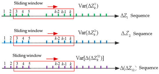
Figure 8.
Sample estimation based on sliding window.
Assuming that the length of the sliding window is , the variance of the involved random sequence is calculated as follows:
where
- (b)
- Forgetting-factor design
In order to ensure the real-time noise tracking, the length of the window should not be too long, but it is easy to cause inaccurate estimation results. In order to solve this contradiction, the method of attenuating memory is adopted, and a forgetting factor is introduced to weigh the historical information. The specific steps are as follows:
where
is the forgetting factor, which is used to adjust the use weight of the observation noise variance matrix at the current time, generally 0.95~0.995, is the direct output of the observed noise variance matrix obtained by SOMD sequence at the current moment, and and are the final estimation results of the noise variance matrix at moment and moment , respectively. The function represents the estimation equation of each algorithm.
- (c)
- Mutation Fault Detection
Considering the real-time nature of the estimation, a finite-length window is used for statistical estimation, so the pollution of the data in the window by the anomalous observations cannot be ignored. In order to suppress the influence of outliers on the estimation of observation noise and improve the accuracy of error estimation, a criterion for anomaly data mining [33] is introduced to detect random errors based on SOMD sequence.
In the case of redundant observation and , if there are outliers in any of the observation,
The detection condition of the anomaly can be designed as
where is the modulus of SOMD vector, and is the standard deviation coefficient used to judge outliers, called confidence level. The smaller the confidence, the stricter the definition of the outlier, which is usually taken as . Due to the stationarity of the statistical properties of noise, the sum of the noise covariance , of the previous moment is substituted for and at the current moment.
As mentioned above, the variance of the error in the INS increment is much smaller than the variance value of the error in LTE; Equation (18) is simplified to the following:
Equation (19) is the confidence interval of SOP/INS observations. This decision condition can be directly implemented in the SOMD noise estimation process in Section 3.4 without introducing additional data and calculation. According to the correlation between track vector and filter track, the singularities in the SOP pseudo-measurement track can be further filtered out, and accurate system positioning results can be obtained.
3.4.2. RMNCE Validation
An analysis of the effect of the noise covariance with the types and influence factors of the measurement noise is shown in Table 3, generally divided into two cases: case 1 is Gaussian hypothesis distribution; case 2 is time-varying noise distribution, where , is the measurement error.
Table 3.
Measurement noise value setting.
Case 1 is the ideal state, is the constant, and case 2 is the distribution of measured noise pollution. The variance of the measured noise measured by each observation of the first set of experiments is a fixed value. The variance of the measured noise varies the observed amount over the selected time interval of the second set of experiments. The simulation results of the time-varying noise covariance and observation measurements in the two cases are shown in Figure 9.
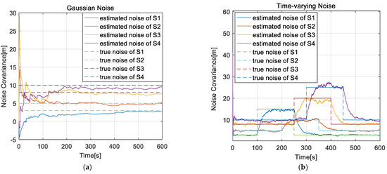
Figure 9.
Measurement noise covariance of different types: (a) the case of Gaussian distribution noise; (b) the case of time-varying noise.
The observation data of 600 samples were used to estimate the noise covariance of four redundant measurements under different types, with a sampling interval of 0.01 s. The above two types of noise can be well realized in a real-time tracking estimation of noise covariance when the noise characteristics of the measurement system were unknown or there is no prior knowledge. In case 1, the measurement converges around 20 s, and the SOMD estimation results converge around the true value quickly; in case 2, the measurement noise variance had been changed between 100 and 450 s, and SOMD can effectively sense the change and realize the estimation of noise covariance. At the same time, case 2 illustrated that the estimations of the noise variance of each dimension of the measurement system by the SOMD algorithm were independent of each other and were not affected by the measurement noise of the other dimensions. The positioning error can be estimated by inputting the above adaptive measurement noise covariance into the navigation model.
Meanwhile, the observation data of 600 samples were used to estimate the noise covariance under different forgetting factors. The measurement 2 parameters in Table 3 were selected to estimate the measurement noise, and the forgetting factors were 0.95, 0.97, and 0.99, respectively. Figure 10 shows the variance of noise covariance. As can be seen from the figure, the larger the noise, the closer was to the real noise, and the estimation effect of noise covariance was better when the factor was 0.99.
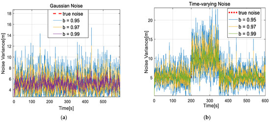
Figure 10.
Measurement noise covariance of different factors: (a) the case of Gaussian distribution noise; (b) the case of time-varying noise.
3.4.3. EKF Framework
For the navigation system, it can be regarded as consisting of two parts, one of which is correctly predicted by the known motion equation, and the other as a random component with zero mean. Considering the difference in INS/SOP integration architecture, the EKF, the unscented Kalman filter (UKF), and the particle filter (PF) are usually used and other nonlinear filters to deal with the nonlinearities of the integrated system. Although the UKF algorithm appears to have considerable advantages over the EKF method, the unknown statistical properties of noise are still a stumbling block to its optimal estimation [34]. Different from the UKF method, which is based on deterministic sampling, the PF method applies a large number of random particles to approximate the posterior density distribution of the state [35] and even requires a heavy computational burden and faces particle degradation and sample poverty in practical applications usually [36]. Since the observed vectors are usually uncorrelated in each dimension, the SOMD algorithm can be used separately in each dimension.
The simulation scene was set where the X-Y axis target moves along a straight line at a constant speed, and the positioning performances using EKF and PF algorithm before and after proposed RMNCE are analyzed. The simulation parameters are seen in Table 4.
Table 4.
Simulation parameters of filtering.
Figure 11 shows the simulation results of filtering track and error based on EKF and PF algorithm. From the analysis of positioning accuracy, it can be shown in Figure 11a, the PF track was closer to the real track, which had obvious advantages, and the positioning RMSE can reach 0.42 m, due to the particles of the PF can be reset after each measurement updating. Considering RMNCE, the positioning accuracy of the two filters had been partially improved, among which the positioning effect of RMNCE PF was better than that of RMNCE EKF; however, the accuracy was higher in several areas, such as Y-axis RMSE, due to the weighting factor of PF being related to the measurement noise and the measurement noise changing constantly. It can be difficult to sample the real distribution, and it occasionally diverged or even failed. From the calculation time, the number of particles used by PF occupies a certain scale; it takes about 30 s for PF and RMNCE PF to process a 500 m measurement track. However, EKF and RMNCE are much faster than 0.01 s, which is obviously advantageous for the real-time navigation. Table 5 was an overview of the simulation time and positioning error of the filters. The above simulation results are ideal, which shows that RMNCE has certain advantages. However, the applicability of this algorithm to most real-world systems is limited because it relies on redundant measurements.
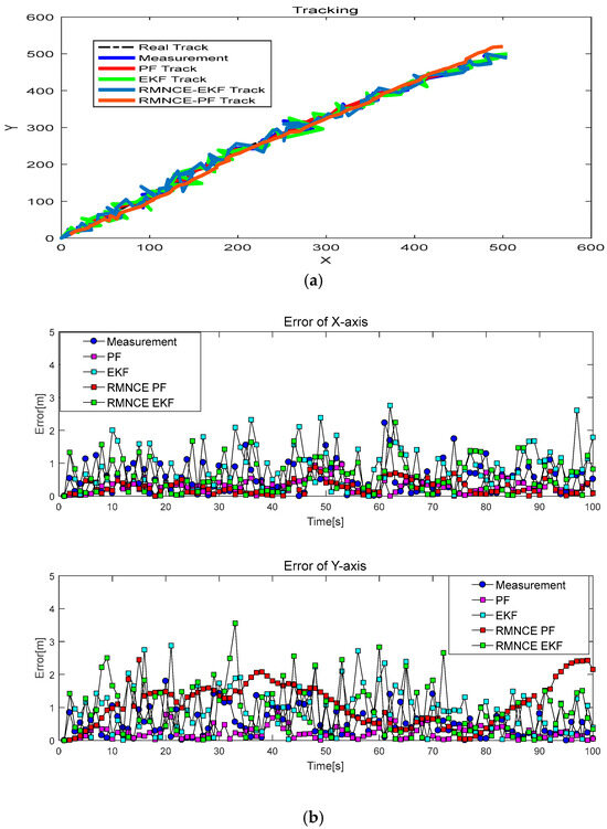
Figure 11.
The filtering effect based on RMNCE: (a) true track and filter estimation; (b) X-Y positioning RMSE.
Table 5.
The simulation times and positioning errors of RMNCE filters.
The research in reference [37] shows that deep learning and other methods can be used to predict the motion state of the carrier more accurately, but considering the computing power and complexity constraints of the platform, EKF is commonly used to estimate and filter. In this paper, the EKF framework based on RMNCE is used to deal with the measurement track.
4. Navigation Model Descriptions
4.1. INS Measurement Model
Different from the conventional GNSS/SINS coupled system, which takes the errors of INS and GNSS as state variables, this paper uses the three-dimensional position and attitude information of INS, the errors of inertial sensor, including the accelerometer and gyroscope, as state input, and the filter uses this information to calculate INS estimation. The form of the state equation is as follows:
where , , and , respectively, represent the position, velocity, and attitude angle of INS carrier, , and represent the error of gyroscope and accelerometer. The subscripts x, y, and z represent the three measurement axes of the carrier coordinate system. The form of the observation equation that takes the coordinate position longitude, latitude, and height as the output is as follows:
The measurement matrix corresponding to the position is .
4.2. SOP Measurement Model
In this paper, we select the LTE signal as the SOP, and the state vector consists of the position and speed estimated by the pseudo-measurement.
represent the target position estimated using the BS, and are the corresponding velocity components.
In Section 3.3, the relationship between the pseudo-range and the position estimation obtained by the path attenuation model is as follows:
where is the distance between the lth BS position and the estimated position, and is the coordinate. Therefore, the observed measurement of SOP at time k can be composed of sampled RSS. Assuming that the number of available base stations at time k is L, it is denoted as follows:
The measurement vector is obtained from the relationship between RSS and distance in Equation (5).
The measurement transfer matrix is as follows:
4.3. SOP/INS Tightly Model
The tight SOP/INS navigation model, which is seen in Appendix C, includes SOP signal pre-processing, filtering update, INS filtering value prediction, and other links.
4.3.1. State and Observation Equation Design
The state equation of the tight SOP/INS model consists of twenty-one-dimensional vectors, expressed as follows:
The estimated position derived from the SOP and INS are incorporated into the measurement equation as follows:
Then, the system measurement matrix is the following:
4.3.2. Robust SOP-Aided Model
A robust combined model is proposed based on the SOP/INS model, and the related methods are seen in Section 3. Once the received-SOP-signal sampling was completed, clock bias correction, multilateral positioning, and RMNCE KF update were carried out. For unknown BS location, the positioning calculation of BS stated that for the case where the statistical characteristics of noise were unknown, the noise covariance was updated using the RMNCE method, and the confidence interval of random error was judged to suppress the influence caused by noise anomalies. The enhanced model structure is shown in Appendix D.
4.3.3. Simulation Result
Assume that the target passes through a densely distributed area LTE macro-station at a constant speed. In a 1000 m × 1000 m area, 16 BSs are randomly generated. The initial X-Y coordinates of the radiation source are [−10, 100]T m, and the simulation time remained at 120 s. As shown in Table 6, the simulation parameters and error parameters of each direct measurement are set according to the velocity measurement, heading measurement of the INS and the radial distance from the target to the BSs.
Table 6.
Parameter setting of SOP-aided model.
According to the set simulation parameters and error parameters, the simulation is carried out with the software MATLAB 2016b, and the results are shown in Figure 12.
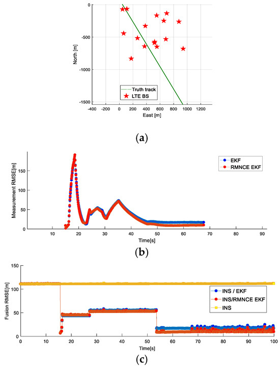
Figure 12.
LTE positioning: (a) motion track and BS position; (b) EKF and RMNCE EKF positioning RMSE; (c) INS and fusionpositioning RMSE.
As can be seen in Figure 12 the RMSE of RMNCE EKF and EKF were close within the 350th sampling point; since then, the RMSE of the RMNCE EKF was significantly smaller than EKF, with a maximum difference of about 8 m. Compared with INS recurrence error, the RMSE of the RMNCE EKF was 10.28 m, which is prior to the performance of EKF, which is 17.42 m.
Reference [32] shows that when only one LTE station and one DTMB station are used for hybrid positioning in an urban environment, the system achieves 26.26 m RMSE over a 162 m trajectory, and accordingly, the threshold of error convergence was set as 25 m. Table 7 shows the error comparison of the RMNCE and EKF methods.
Table 7.
Parameter setting of SOP-aided model.
After pseudo-measurement filtering, the track can converge within 20 m, and the positioning accuracy of the enhanced model is smaller than that of EKF. In addition, the SOP-assisted positioning can significantly improve the cumulative error of INS, and the EKF and RMNCE navigation can be improved by 85% and 91%, respectively, compared with a single INS navigation in the absence of GNSS.
5. Experiment and Analysis
5.1. Experimental Method
Taking the collected LTE signal as an example, the vehicle-mounted platform is used to verify the data acquisition and positioning calculation functions of the robust SOP/INS navigation model. The prototype equipment was assembled as shown in Figure 13, including omnidirectional antenna, radio-monitoring receiver, terminal processor, and power supply equipment.
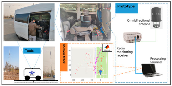
Figure 13.
On-board experiment of NAVSOP.
The experimental steps are as follows.
- The acquisition software sets the receiver bandwidth at 28 MHz and signal sampling central frequency at , and records the signal amplitude and current latitude and longitude information of the software interface.
- IQ data are dynamically sampled during the carrier march, and the data are transmitted to the terminal and recorded.
- Adjust the sampling frequency at on the sampling software and repeat step 2.
- Run the positioning solution program of the data processing terminal, and analyze the positioning results with reference to INS track and GPS.
5.2. Platform and Route
The data collection site is from south to north Qingyuan Street, Fangshan District, Beijing, and signals from seven LTE BSs are received along the way. The platform shown in Figure 14 is driven in a straight line at constant speed of 60 km/h in the urban environment of Fangshan District, Beijing, China. It was equipped with a radio receiver with an RSS recording function, and the data acquisition time was a continuous 17 s. The line runs from north to south along Qingyuan North Street, including A and B marker points. Table 8 shows the platform parameters and the detected LTE BS locations. Here, the latitude and longitude of the starting point were E 116.195092° and N 39.730360°, and its coordinate was set as [0, 0]T. The BS positions were given by latitude and longitude, and Cart coordinates can be obtained by transformation.
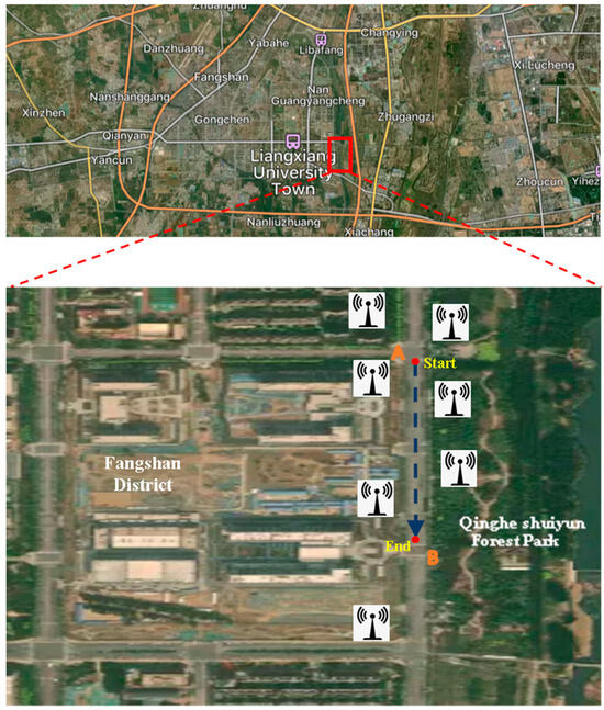
Figure 14.
On-board test route.
Table 8.
On-board test parameter setting.
5.3. On-Board Test Result
The test result can be seen in Figure 15. From Figure 15a, the RSS indicators of seven BSs ranged from −110 dB to −80 dB; from Figure 15b, the existing RSS noises caused the singularity of the pseudo-measurement when passing through the dense areas. After filtering, the track error began to converge at 7.5 s, the maximum and minimum error from convergence to the end were 12.96 m and 10.39 m, respectively, and the positioning RMSE of the navigation system was 11.68 m.
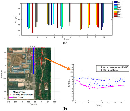
Figure 15.
On-board test results: (a) average RSS indicators of each BS; (b) motion trajectories and positioning errors.
In Ref. [32], the DTMB signal and LTE signal were used for hybrid positioning in the urban environment, and the RMSE was 23.17 m on a 600 m track, as only four LTE BSs were used. We analyzed the positioning performance of the two from the number of BSs, the length of trajectory, and positioning RMSE in Table 9. From the results, the positioning accuracy of the proposed method was better than that of reference [32] with the similar number of BSs.
Table 9.
Statistics of positioning-test results.
6. Conclusions
In the case of GNSS denial, commercial SOPs are abundant in most urban areas, with the advantages of wide-frequency-band distribution, wide transmission range, fast construction speed, strong recovery, and, most importantly, they can be used for free. Limited by the storage space of the acquisition device, this paper only verifies that NAVSOP fusion positioning in a very short trajectory. Regardless, it is very promising and valuable.
When the statistical characteristics of noise are unknown, the noise estimation method based on redundant measurement SOMD is extended to the application scenario that can objectively describe the measurement noise of arbitrary signal, and the dependence on observation information is reduced. This estimation of the noise covariance R expands and enriches the adaptive filtering system. The simulation results show that the SOP-assisted positioning can significantly improve the cumulative error by INS, and the RMNCE method improves 91% compared with single INS navigation. In addition to the roadster test, the accuracy of the SOP-assisted robust navigation model reached 11.68 m over a 283 m trajectory.
This study has certain limitations: (1) The current simulation model and positioning accuracy are suitable for a two-dimensional plane in the X-Y coordinate system; future research could focus on positioning models that account for changes in height. (2) The multilateral positioning algorithm is not applicable when the number of BSs is less than 3, and improvements need to be made for such situations. (3) The validation scenario only analyzed a multi-base station environment in urban settings; although the intensity path loss numerical model used has a certain resistance to multipath effects, further exploration of more extreme usage scenarios is needed to verify the adaptability of the algorithm.
Author Contributions
Conceptualization, H.Z.; methodology, L.Z. and H.Z.; software, A.W.; validation, A.W.; formal analysis, C.T.; writing—original draft, L.Z.; writing—review and editing, C.T. All authors have read and agreed to the published version of the manuscript.
Funding
This study was partly supported by China National Key Research and Development Program under Grant 2017YFC0821102 and Grant 2016YFB0502004.
Data Availability Statement
The data that support the findings of this study are available on request from the corresponding author, [Hai Zhang], upon reasonable request.
Conflicts of Interest
The authors declare no conflicts of interest.
Appendix A. LTE Location Information Extraction Method
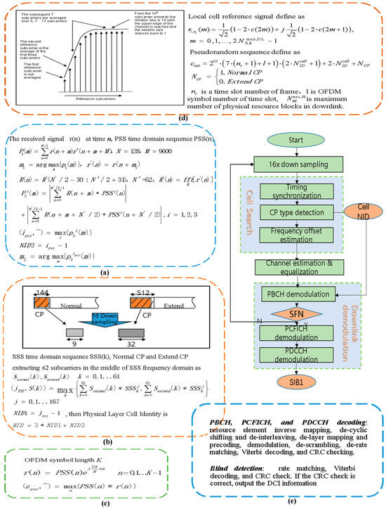
Figure A1.
LTE downlink signal solution: (a) timing synchronization; (b) CP type detection; (c) frequency offset estimation; (d) channel estimation; (e) downlink demodulation.
Appendix B. Multilateral Positioning Method
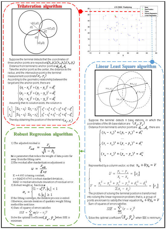
Figure A2.
Multilateral positioning based on distance: Trilateral location algorithm (red); Least squares positioning algorithm (blue); Robust regression positioning algorithm (green).
Appendix C. Tightly SOP/INS Navigation Model
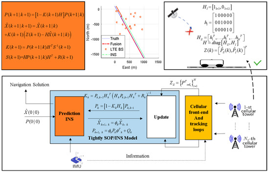
Figure A3.
Tightly SOP/INS navigation model: SOP signal pre-processing, filtering update, INS filtering value prediction, and other links.
Appendix D. Robust NAVSOP Model
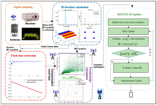
Figure A4.
Robust NAVSOP model: BS location calculation, clock bias correction, pseudo-range calculation, and RMNCE EKF update.
References
- Grenier, A.; Lohan, E.S.; Ometov, A.; Nurmi, J. Towards Smarter Positioning through Analyzing Raw GNSS and Multi-Sensor Data from Android Devices: A Dataset and an Open-Source Application. Electronics 2023, 12, 4781. [Google Scholar] [CrossRef]
- Gao, L.; Battistelli, G.; Chisci, L.; Wei, P. Distributed Joint Sensor Registration and Multitarget Tracking via Sensor Network. IEEE Trans. Aerosp. Electron. Syst. 2020, 56, 1301–1317. [Google Scholar] [CrossRef]
- Xiao, Z.; Yang, D.; Wen, F.; Jiang, K. A Unified Multiple-Target Positioning Framework for Intelligent Connected Vehicles. Sensors 2019, 19, 1967. [Google Scholar] [CrossRef] [PubMed]
- Liu, F.; Han, H.; Cheng, X.; Li, B. Performance of Tightly Coupled Integration of GPS/BDS/MEMS-INS/Odometer for Real-Time High-Precision Vehicle Positioning in Urban Degraded and Denied Environment. J. Sens. 2020, 2020, 1–15. [Google Scholar] [CrossRef]
- Farhangian, F.; Landry, R., Jr. Multi-Constellation Software-Defined Receiver for Doppler Positioning with LEO Satellites. Sensors 2020, 20, 5866. [Google Scholar] [CrossRef]
- Ning, C.; Li, R.; Li, K. Outdoor Location Estimation Using Received Signal Strength-Based Fingerprinting. Wirel. Pers. Commun. 2016, 89, 365–384. [Google Scholar] [CrossRef]
- Ding, J.; Wang, J.; Zhang, Y.; Li, Y.; Zheng, N. Correlation-Based Robust Linear Regression with Iterative Outlier Removal. In Proceedings of the ICASSP 2021—2021 IEEE International Conference on Acoustics, Speech and Signal Processing (ICASSP), Toronto, ON, Canada, 6–11 June 2021; pp. 5594–5598. [Google Scholar] [CrossRef]
- Diskin, T.; Draskovic, G.; Pascal, F.; Wiesel, A. Deep robust regression. In Proceedings of the 2017 IEEE 7th International Workshop on Computational Advances in Multi-Sensor Adaptive Processing (CAMSAP), Curaçao, The Netherlands, 10–13 December 2017; pp. 1–5. [Google Scholar] [CrossRef]
- Vouch, O.; Minetto, A.; Falco, G.; Dovis, F. On the Adaptivity of Unscented Particle Filter for GNSS/INS Tightly-Integrated Navigation Unit in Urban Environment. IEEE Access 2021, 9, 144157–144170. [Google Scholar] [CrossRef]
- Zhang, H.; Chang, Y.H.; Che, H. Measurement-based adaptive kalman filtering algorithm for GPS/INS integrated navigation system. J. Chin. Inert. Technol. 2010, 18, 696–701. [Google Scholar]
- Jiang, L.; Zheng, G.; Zhang, B. A Noise Estimation Method Based on Envelope Pseudo-measurement System in Adaptive Kalman Filter. In Proceedings of the 2024 43rd Chinese Control Conference (CCC), Kunming, China, 28–31 July 2024; pp. 208–213. [Google Scholar] [CrossRef]
- Driusso, M.; Marshall, C.; Sabathy, M.; Knutti, F.; Mathis, H.; Babich, F. Vehicular Position Tracking Using LTE Signals. IEEE Trans. Veh. Technol. 2016, 66, 3376–3391. [Google Scholar] [CrossRef]
- Gebre-Egziabher, D. GNSS Solutions—Inside GNSS. Inside GNSS 2011, 22–27. Available online: https://insidegnss-com.exactdn.com/wp-content/uploads/2018/01/IGM_janfeb11-Solutions.pdf (accessed on 12 February 2025).
- Morales, J.J.; Kassas, Z.M. Tightly Coupled Inertial Navigation System With Signals of Opportunity Aiding. IEEE Trans. Aerosp. Electron. Syst. 2021, 57, 1930–1948. [Google Scholar] [CrossRef]
- Maaref, M.; Kassas, Z.M. Autonomous Integrity Monitoring for Vehicular Navigation With Cellular Signals of Opportunity and an IMU. IEEE Trans. Intell. Transp. Syst. 2021, 23, 5586–5601. [Google Scholar] [CrossRef]
- Du, J.; Diouris, J.-F.; Wang, Y. A RSSI-based parameter tracking strategy for constrained position localization. EURASIP J. Adv. Signal Process. 2017, 2017, 77. [Google Scholar] [CrossRef]
- Akhpashev, R.V.; Andreev, A.V. COST 231 Hata adaptation model for urban conditions in LTE networks. In Proceedings of the 2016 17th International Conference of Young Specialists on Micro/Nanotechnologies and Electron Devices (EDM), Erlagol, Russia, 30 June–4 July 2016; pp. 64–66. [Google Scholar]
- Ding, J.; Liu, Y.; Liao, H.; Sun, B.; Wang, W. Statistical Model of Path Loss for Railway 5G Marshalling Yard Scenario. ZTE Commun. 2023, 21, 117–122. [Google Scholar]
- Schirru, L.; Lodi, M.B.; Fanti, A.; Mazzarella, G. Improved COST 231-WI Model for Irregular Built-Up Areas. In Proceedings of the 2020 XXXIIIrd General Assembly and Scientific Symposium of the International Union of Radio Science, Rome, Italy, 29 August–5 September 2020; pp. 1–4. [Google Scholar]
- Thrane, J. Optimisation of Future Mobile Communication Systems Using Deep Learning. Ph.D. Thesis, Technical University of Denmark, Kongens Lyngby, Denmark, 2020; pp. 63–72. [Google Scholar]
- Lee, D.J.; Lee, W.C. Enhanced Lee In-Building Model. In Proceedings of the 2013 IEEE 78th Vehicular Technology Conference (VTC Fall), Las Vegas, NV, USA, 2–5 September 2013; pp. 1–6. [Google Scholar]
- Federal Communications Commission Report on the Expansion of Flexible Use in Mid-Band Spectrum Between 3.7 and 24 GHz. Available online: https://docs.fcc.gov/public/attachments/FCC-23-86A1.pdf (accessed on 12 February 2025).
- Stuhlfauth, R. 5G NTN Takes Flight: Technical Overview Of 5G Non-Terrestrial Networks. In White Paper V0.100; Rohde & Schwarz: Munich, Germany, 2022; p. 67. [Google Scholar]
- Hegarty, C.; Kaplan, E. Understanding GPS Principles and Applications, 2nd ed.; Artech: London, UK, 2005. [Google Scholar]
- Jiang, L.; Zhang, H. Redundant measurement-based second order mutual difference adaptive Kalman filter. Automatica 2018, 100, 396–402. [Google Scholar] [CrossRef]
- Fitzgerald, R. Divergence of the Kalman filter. IEEE Trans. Autom. Control. 1971, 16, 736–747. [Google Scholar] [CrossRef]
- 3GPP TS 36.101; Evolved Universal Terrestrial Radio Access (E-UTRA), User Equipment (UE) Radio Transmission and Reception. Available online: https://www.etsi.org/deliver/etsi_ts/136100_136199/136101/08.26.00_60/ts_136101v082600p.pdf (accessed on 12 February 2025).
- Hamid, M.; Kostanic, I. Path Loss Models for LTE and LTE-A Relay Stations. Univers. J. Commun. Netw. 2013, 1, 119–126. [Google Scholar] [CrossRef]
- Wang, Y.; Ho, K.C. An Asymptotically Efficient Estimator in Closed-Form for 3-D AOA Localization Using a Sensor Network. IEEE Trans. Wirel. Commun. 2015, 14, 6524–6535. [Google Scholar] [CrossRef]
- Farebrother, R.W. Least Absolute Residuals Procedure. In International Encyclopedia of Statistical Science; Lovric, M., Ed.; Springer: Berlin/Heidelberg, Germany, 2011. [Google Scholar]
- Wilcox, R.R.; Keselman, H.J. Robust Regression Methods: Achieving Small Standard Errors When There Is Heteroscedasticity. Underst. Stat. 2004, 3, 349–364. [Google Scholar] [CrossRef]
- Hong, T.; Sun, J.; Jin, T.; Yi, Y.; Qu, J. Hybrid Positioning With DTMB And LTE Signals. In Proceedings of the 2021 International Wireless Communications and Mobile Computing (IWCMC), Harbin City, China, 28 June–2 July 2021; pp. 303–307. [Google Scholar]
- Khisamiev, A.N. Universal Functions and KΣ-Structures. Sib. Math J. 2020, 61, 552–562. [Google Scholar] [CrossRef]
- Zhe, J.; Qi, S.; He, Y.; Han, J. Anovel adaptive unscented Kalman filter for nonlinear estimation. In Proceedings of the 46th IEEE Conference on Decision and Control, New Orleans, LA, USA, 12–14 December 2007. [Google Scholar]
- Wang, X.; Pan, Q.; Huang, H.; Gao, A. Overview of deterministic sampling filtering algorithms for nonlinear system. Control Decis. 2012, 27, 801–812. [Google Scholar]
- Pardal, P.C.P.M.; Kuga, H.K.; de Moraes, R.V. The Particle Filter Sample Impoverishment Problem in the Orbit Determination Application. Math. Probl. Eng. 2015, 2015, 168045. [Google Scholar] [CrossRef]
- Meimetis, D.; Daramouskas, I.; Perikos, I.; Hatzilygeroudis, I. Real-time multiple object tracking using deep learning methods. Neural Comput. Applic 2023, 35, 89–118. [Google Scholar] [CrossRef]
Disclaimer/Publisher’s Note: The statements, opinions and data contained in all publications are solely those of the individual author(s) and contributor(s) and not of MDPI and/or the editor(s). MDPI and/or the editor(s) disclaim responsibility for any injury to people or property resulting from any ideas, methods, instructions or products referred to in the content. |
© 2025 by the authors. Licensee MDPI, Basel, Switzerland. This article is an open access article distributed under the terms and conditions of the Creative Commons Attribution (CC BY) license (https://creativecommons.org/licenses/by/4.0/).