Adaptive Step Size Linear Multistep Method for Small Signal Stability Analysis in Power Systems with Time Delays

Abstract

Distributed energy resources (DERs) offer a promising solution for enhancing the resilience and efficiency of modern power systems. However, the inherent time delays in their communication and control systems can degrade their small signal stability, affecting reliable operation. This paper presents an Adaptive Step Size Linear Multistep Method (AS-LMS), for analyzing small signal stability of the system in the presence of time delays. The AS-LMS automatically adjusts the step size based on the computed solution behavior, achieving a balance between accuracy and computational efficiency. The essential idea is to use smaller steps in regions where the dynamic is changing rapidly and larger steps in regions where it is relatively smooth. Two adaptive step size strategies are proposed. The first strategy compares the current step size to the initial step size, ensuring consistency across iterations. The second strategy compares the current step size with the previous step size, allowing for more local adjustments throughout the numerical integration process. We evaluate the performance of the proposed AS-LMS method on two standard testing systems, i.e., the IEEE 9-bus and IEEE 30-bus systems. Both systems are modified to converter-interfaced DER units and different delays are applied to each testing system. The results show that the proposed AS-LMS method improves computational efficiency while maintaining accuracy in stability assessments. By balancing the accuracy and computational efficiency, the AS-LMS method provides a potent tool to analyze the stability of power systems with time delay.

1. Introduction

Microgrids are emerging as pivotal components in modern power systems due to their ability to enhance resilience, efficiency, and sustainability [1,2]. Unlike traditional centralized power grids, microgrids are decentralized systems consisting of distributed energy resources (DERs), energy storage devices, and loads [3,4]. They can operate autonomously or in conjunction with the main grid, reducing reliance on fossil fuels, mitigating greenhouse gas emissions, and improving energy security. DERs are highly sensitive to time delays due to their reliance on communication systems for coordination and control [5]. Time delays can occur during data transmission between DER units and the central controller, as well as within control actions, such as voltage and frequency regulation [6,7]. These delays affect the stability and performance of the grid, leading to issues such as oscillations, inaccurate synchronization, or even system failure in extreme cases.

Small signal stability analysis is essential for ensuring the reliable operation of power systems, including microgrids. It involves assessing the system’s dynamic response to small disturbances around its operating point. This analysis is crucial for predicting transient behavior, damping oscillations, and maintaining synchronism under varying operating conditions. However, due to the distributed nature of microgrids and the use of communication networks for coordination and control, time delays can be particularly pronounced. Time delays can arise from signal processing and data transmission. Time delays in communication and control systems within microgrids pose significant challenges to small signal stability [8,9,10]. Delays can exacerbate instability, leading to oscillations, voltage fluctuations, and potential system-wide blackouts if not managed properly [11,12,13]. As modern power systems increasingly incorporate DERs and smart grid technologies, the impact of communication and control delays becomes more significant, highlighting the need for methods that effectively account for these delays in dynamic system analysis.

In power system stability studies, Differential-Algebraic Equations (DAEs) and small signal stability analysis are deeply interconnected. DAEs are used to model the dynamic behavior of power systems, which include both differential components, such as generator dynamics, and algebraic components, such as power flow constraints. These equations capture the essential interactions between the dynamic and static elements of the grid. To perform small signal stability analysis on systems modeled by DAEs, the nonlinear DAE system is linearized around an operating point. The resulting linearized system is then used to compute the eigenvalues of the system’s state matrix. The locations of these eigenvalues in the complex plane determine the stability of the system. Eigenvalues with positive real parts indicate instability, while those with negative real parts signify that the system will return to equilibrium after a disturbance. Including time delays in the system modeling leads to formulation of a delayed differential algebraic equation (DDAE). It is more complicated to study the stability of DDAE, i.e., computing the eigenvalues of the linearized DDAE model, because the corresponding characteristic equation will be transcendental.

Existing literature has explored small signal stability analysis in power systems. The impact of time delay on system stability can be analyzed through the use of control theory and mathematical modeling [14,15]. Several methods have been proposed to analyze the small signal stability of power systems with inclusion of delays [16,17,18]. For instance, the Chebyshev discretization [16] was developed to transform the original DDAE problem into an equivalent partial derivative equation (PDE) of infinite dimensions, and solve a finite matrix eigenvalue problem of the discretized PDE. This approach can lead to large system matrices, making the computational process both memory and time intensive. The Padé approximant [17] was utilized to replace the transcendental terms in the characteristic equation, facilitating the computation of eigenvalues for stability analysis in systems with time delays. This approach is sensitive to the order selected for the approximation. Higher-order discretizations may yield greater accuracy, but they can also amplify numerical errors. The Linear Multistep Method was used to solve the eigenvalues of the DDAE [18] and the delayed differential equation (DDE) [19], but the accuracy cannot guaranteed with a large step size or the computational effort is high with a small step size. Overall, traditional methods often assume negligible delays or employ fixed step sizes, which may not capture the complexities of real-world systems. Recent research in power system stability analysis target the challenge of accounting for communication time delays in DERs. Accurate and efficient techniques are thus essential to incorporate time delays into stability analysis.

To bridge the gap, we propose an Adaptive Step Size Linear Multistep Method (AS-LMS) for analyzing small signal stability in power systems with time delays. This method dynamically adjusts the integration step size based on system dynamics, improving computational efficiency while maintaining accuracy.

Microgrids are indeed poised to become a cornerstone of smart cities, renewable energy management, and decentralized power systems, where communication and control delays present significant challenges. The AS-LMS offers potential improvements in analyzing such delays, thereby enhancing the reliability of microgrids. To ensure the applicability of the proposed algorithms in real-time systems, several practical constraints must be considered, particularly in terms of computational resources required for handling large matrices. As the number of state variables and generators increases, the size of the matrix grows rapidly, which demands substantial memory and computational power to perform the necessary calculations. While the AS-LMS method significantly reduces computational effort compared to conventional LMS approaches, the overall computational resource requirements still increase as the system size grows. In real-time applications, the algorithm’s speed and efficiency are crucial to maintaining system stability and performance. The growing size of the system leads to increased computational burden for matrix operations, such as inversion and multiplication, which can lead to longer processing times and may exceed the available resources in typical real-time computing environments. Additionally, hardware limitations, including available processing power and memory, must be carefully considered when implementing the algorithm in real-time systems to ensure efficient operation within the system’s resource constraints.

The novelty of this approach lies in its ability to efficiently and accurately resolve the small-signal stability of time-delayed microgrids. The AS-LMS automatically increases or decreases the step size based on the system’s dynamics, achieving a balance between accuracy and computational efficiency. This is crucial for ensuring the reliable operation of future smart microgrids, which are expected to incorporate increasing levels of DERs, dynamic control systems, and communication-based control loops. By leveraging the strengths of AS-LMS methods, this work provides a robust tool for researchers and engineers to better understand and manage the stability challenges posed by time delays.

The remainder of this paper is organized as follows: Section 2 presents the system modeling with the consideration of time delays, introducing the challenges of analyzing systems with time delays. Section 3 introduces the Linear Multistep Method and the proposed Adaptive Step Size Linear Multistep method. Section 4 provides the numerical examples. Conclusions are drawn in Section 5.

2. System Modeling

2.1. Preliminary Modeling of Systems Without Delays

The transient behavior of a microgrid integrated with DERs can be described through a set of differential-algebraic equations (DAEs) as follows [20,21,22,23], with more details given in the Appendix A.

$$\dot{\mathbf{x}}=\mathbf{F}(\mathbf{x},\mathbf{y},\mathbf{u}),$$

(1)

$$\mathbf{0}=\mathbf{G}(\mathbf{x},\mathbf{y},\mathbf{u}),$$

(2)

where $\mathbf{x}\in {\mathbb{R}}^n$ is the state variable vector, i.e., state variables in the controller of DER power-electronic interfaces, $\mathbf{y}\in {\mathbb{R}}^m$ is the algebraic variable vector, i.e., bus voltage amplitude and angle, line currents, and $\mathbf{u}\in {\mathbb{R}}^p$ represents the input variations or disturbances, e.g., power output fluctuation of the DERs and power load changes.

2.2. System Modeling with Delays

Introducing delays to (1) and (2) leads to a set of DDAE. Consider the case of constant time delays in the form (3) and (4),

$${\mathbf{x}}_d=\mathbf{x}(t-\tau ),$$

(3)

$${\mathbf{y}}_d=\mathbf{y}(t-\tau ),$$

(4)

where ${\mathbf{x}}_d$ is the delayed variable with respect to the state variable $\mathbf{x}$, t is the current simulation time, and $\tau$ is the delay, ${\mathbf{y}}_d$ is the delayed variable with respect to the algebraic variable $\mathbf{y}$. Then, the modeling in (1) and (2) can be revised as follows [24],

$$\dot{\mathbf{x}}=\mathbf{F}(\mathbf{x},\mathbf{y},{\mathbf{x}}_d,{\mathbf{y}}_d,\mathbf{u}),$$

(5)

$$\mathbf{0}=\mathbf{G}(\mathbf{x},\mathbf{y},{\mathbf{x}}_d,{\mathbf{y}}_d,\mathbf{u}).$$

(6)

Note that the system described in (5) and (6) represents the most general form of DDAEs. However, in practical applications, ${\mathbf{y}}_d$ can often be ignored because delayed algebraic variables typically have minimal impact on system dynamics, unlike delayed differential states, which are critical for stability analysis. Simplified models of the physical systems corresponding to (7) and (8) can then be employed [16].

$$\dot{\mathbf{x}}=\mathbf{F}(\mathbf{x},\mathbf{y},{\mathbf{x}}_d,{\mathbf{y}}_d,\mathbf{u}),$$

(7)

$$\mathbf{0}=\mathbf{G}(\mathbf{x},\mathbf{y},{\mathbf{x}}_d,\mathbf{u}).$$

(8)

To perform the small signal stability, we linearize the system around its equilibrium point, as given in (9).

$$\Delta \dot{\mathbf{x}}={\mathbf{A}}_0\Delta \mathbf{x}+\sum _{j=1}^n{\mathbf{A}}_j\Delta \mathbf{x}(t-{\tau }_j)+\sum _{e=1,r=e}^n{\overline{\mathbf{A}}}_{e,r}\Delta \mathbf{x}(t-{\tau }_{e,r}),$$

(9)

where,

$${\tau }_{e,r}={\tau }_e+{\tau }_r\mathrm{for}e=1,2,\cdots ,n,r=e,\cdots ,n,$$

(10)

and

$${\overline{\mathbf{A}}}_{e,r}=\left\{\begin{array}{c}-{\mathbf{F}}_{y_{d,e}}{\mathbf{G}}_y^{-1}{\mathbf{G}}_{x_{d,e}},\mathrm{for}\mathrm{e}=\mathrm{r},\hfill \\ -{\mathbf{F}}_{y_{d,e}}{\mathbf{G}}_y^{-1}{\mathbf{G}}_{x_{d,r}}-{\mathbf{F}}_{y_{d,r}}{\mathbf{G}}_y^{-1}{\mathbf{G}}_{x_{d,e}},\mathrm{for}\mathrm{e}\ne \mathrm{r}.\hfill \end{array}\right.$$

(11)

Define ${\overline{\mathbf{A}}}_{e,r}$ in terms of ${\mathbf{A}}_k$ through (12),

$${\mathbf{A}}_k={\overline{\mathbf{A}}}_{e,r},\mathrm{where}k=e·n+r-\sum _{e=1}^e(e-1).$$

(12)

Combine (9), (10) and (12) to get (13),

$$\Delta \dot{\mathbf{x}}={\mathbf{A}}_0\Delta \mathbf{x}+\sum _{j=1}^n{\mathbf{A}}_j\Delta \mathbf{x}(t-{\tau }_j)+\sum _{k=n+1}^{n+m}{\mathbf{A}}_k\Delta \mathbf{x}(t-{\tau }_k),$$

(13)

where,

$${\mathbf{A}}_j={\mathbf{F}}_{x_{d,j}}-{\mathbf{F}}_y{\mathbf{G}}_y^{-1}{\mathbf{G}}_{x_{d,j}}-{\mathbf{F}}_{y_{d,j}}{\mathbf{G}}_y^{-1}{\mathbf{G}}_x,$$

(14)

$${\mathbf{A}}_k=-{\mathbf{F}}_{y_{d,e}}{\mathbf{G}}_y^{-1}{\mathbf{G}}_{x_{d,e}},\mathrm{for}\mathrm{e}=\mathrm{r},$$

(15)

$${\mathbf{A}}_k=-{\mathbf{F}}_{y_{d,e}}{\mathbf{G}}_y^{-1}{\mathbf{G}}_{x_{d,r}}-{\mathbf{F}}_{y_{d,r}}{\mathbf{G}}_y^{-1}{\mathbf{G}}_{x_{d,e}},\mathrm{for}\mathrm{e}\ne \mathrm{r},$$

(16)

$${\tau }_k={\tau }_{e,r},\mathrm{where}k=e·n+r-\sum _{e=1}^e(e-1).$$

(17)

In (14), j indicates the index of the delays that exist in the system. In (15) and (16), k indicates the index of the delays that are generated during the computational process. ${\mathbf{F}}_x$ and ${\mathbf{G}}_x$ are matrices of partial derivatives of the state variables, ${\mathbf{F}}_y$ and ${\mathbf{G}}_y$ are matrices of partial derivatives of the algebraic variables, ${\mathbf{A}}_0$ is the state matrix, ${\mathbf{A}}_j$ and ${\mathbf{A}}_k$ are the delayed state matrices. Denote v as the total number of delays, i.e., v = n + m. Rewrite (13) in (18) to simplify.

$$\Delta \dot{\mathbf{x}}={\mathbf{A}}_0\Delta \mathbf{x}+\sum _{i=1}^v{\mathbf{A}}_i\Delta \mathbf{x}(t-{\tau }_i),$$

(18)

where ${\mathbf{A}}_i$ is the delayed state matrix that corresponds to the i-th delay in the microgrid system.

It is essential to calculate the eigenvalues of (18) to analyze the small signal stability, where the characteristic equation that describes the stability of (18) can be expressed in (19),

$$\det \Delta \left(\lambda \right)=\mathbf{0},$$

(19)

where the characteristic matrix is

$$\Delta \left(\lambda \right)=\lambda {\mathbf{I}}_n-{\mathbf{A}}_0-\sum _{i=1}^v{\mathbf{A}}_{\mathbf{i}}{e}^{-\lambda {\tau }_i},$$

(20)

where ${\mathbf{I}}_n$ is the identity matrix of order n, $\lambda$ is the eigenvalue.

Note that the solution of the characteristic Equation (19) is transcendental, which means that there will be infinitely many roots, typically we are only able to determine a subset of the approximated numerical solutions. To overcome the difficulty of computational complexity and solve the eigenvalues efficiently and accurately, an adaptive step size linear multiple step size method (AS-LMS) is proposed below.

3. Adaptive Step Size Linear Multistep Method

Linear Multistep methods (LMS) are a class of numerical methods used for solving ordinary differential equations (ODEs) [19]. They involve using a combination of past and present steps to approximate the solutions in future time steps. These methods are especially useful for solving ODEs that involve time delays, as they allow for the explicit incorporation of the delayed terms into the numerical scheme.

LMS methods can be used to solve DDAEs by discretizing the delayed terms using a step size, h. The delayed terms can then be approximated using a linear combination of past and present values of the solution. The LMS methods are employed for solving stiff and delay-differential equations, which are prevalent in the stability analysis of time-delayed systems. LMS ensures numerical stability while effectively capturing the rightmost eigenvalues, which are critical for small-signal stability analysis.

The size of the resulting eigenvalue problem is inversely proportional to h used in the discretization. The choice of h is a critical aspect of this technique. If the step size is too large, the errors may accumulate quickly. If the step size is too small, the computational cost may become prohibitively high. In order to balance the size of the problem and the accuracy of the solutions, an Adaptive Step Size LMS (AS-LMS) method is developed. The AS-LMS adjusts the step size dynamically based on the solution behavior, which can improve the accuracy while reducing the computational cost.

3.1. General LMS Algorithm

The general form of a c-step formula of a LMS method that is applied to (18) is shown in (21) [25].

$$\sum _{j=0}^c{\alpha }_j\Delta {\mathbf{x}}_{L+j}=h\sum _{j=0}^c{\beta }_j({\mathbf{A}}_0\Delta {\mathbf{x}}_{L+j}+\sum _{i=1}^v{\mathbf{A}}_i\Delta \tilde{\mathbf{x}}(t_{L+j}-{\tau }_i)),$$

(21)

where L is arbitrary time step, $\Delta \tilde{\mathbf{x}}(t_{L+j}-{\tau }_i)$ is the approximation of $\Delta \mathbf{x}(t_{L+j}-{\tau }_i)$ obtained from the preciously computed mesh points $\Delta {\mathbf{x}}_{L+l}$, $l<j$, which is the Nordsieck interpolation as given in (22),

$$\Delta \tilde{\mathbf{x}}(t_L-ϵh)=\sum _{l=-L_{-}}^{L_{+}}\left(\prod _{o=-L_{-},o\ne l}^{L_{+}}\left({\displaystyle \frac{ϵ-o}{l-o}}\right)\Delta {\mathbf{x}}_{L+l}\right),$$

(22)

where,

$$ϵ=\lceil {\displaystyle \frac{\tau }{h}}\rceil -{\displaystyle \frac{\tau }{h}}\in [0,1),$$

(23)

and $h=t_{L+j+1}-t_{L+j}$ is a fixed step size, ${\alpha }_j$ and ${\beta }_j$ are the coefficients of the LMS method, they are designed to get a good approximation of the value of $\Delta {\mathbf{x}}_{L+j}$ [25]. The design of the coefficients ${\alpha }_j$ and ${\beta }_j$ in (21) is crucial for ensuring that the method closely approximates the true solution while remaining easy to apply. In many cases, some coefficients are set to zero to simplify the method without significantly affecting the accuracy. With ${\alpha }_c=1$ in (21), the coefficients ${\alpha }_0,\cdots ,{\alpha }_{c-1}$ and ${\beta }_0,\cdots ,{\beta }_c$ determine the method. Various families of multistep methods are commonly employed, including Adams-Bashforth methods [25], Adams-Moulton methods [25], and Backward Differentiation Formula methods [26], each offering distinct characteristics. These methods can be classified as explicit or implicit based on the value of ${\beta }_c$. If ${\beta }_c=0$, the method is explicit, where the solution at each step is determined using only past values. If ${\beta }_c\ne 0$, the method is implicit, requiring the solution of a system of equations that involve future values. During time integration, (21) is solved for $\Delta {\mathbf{x}}_{L+c}$ (for successive values of L) based on the previously computed mesh points.

Assume the matrix $\mathbf{M}$ in (24) denotes the Jacobian of (21), then the root of $\mathbf{M}$, $\sigma$, can be used to determine the eigenvalues of (18), i.e., the exponential transformation in (26) maps eigenvalue $\lambda$ to $\sigma$.

$$\left[\begin{array}{c}\Delta x_{L-\lceil {\displaystyle \frac{{\tau }_i}{h}}\rceil +1}\\ \Delta x_{L-\lceil {\displaystyle \frac{{\tau }_i}{h}}\rceil +2}\\ ⋮\\ \Delta x_{L+c}\end{array}\right]=\mathbf{M}\left[\begin{array}{c}\Delta x_{L-\lceil {\displaystyle \frac{{\tau }_i}{h}}\rceil }\\ \Delta x_{L-\lceil {\displaystyle \frac{{\tau }_i}{h}}\rceil +1}\\ ⋮\\ \Delta x_{L+c-1}\end{array}\right],$$

(24)

where,

$$\mathbf{M}=[{\mathbf{M}}_1{\mathbf{M}}_2\cdots {\mathbf{M}}_{\mathcal{N}}],\mathcal{N}=\lceil {\displaystyle \frac{c+1}{h}}\rceil ,$$

(25)

with each ${\mathbf{M}}_{\mathcal{I}}$ being a n by n matrix for $\mathcal{I}$ = 1, 2, ⋯, $\mathcal{N}$.

$$\sigma =exp\left(h\lambda \right).$$

(26)

In other words, the LMS method is used to compute the eigenvalues $\sigma$ of the matrix $\mathbf{M}$ for $\Delta x_{L+c}$. Afterward, a shift transformation is applied to obtain the eigenvalues, $\lambda$.

3.2. Adaptive Step Size LMS (AS-LMS)

The AS-LMS in (27) is an extension of the general LMS. It adapts the step size based on the previous step solutions, and allows for automatic adjustment of the step size during the numerical integration process. This approach helps improve the accuracy and efficiency of the numerical integration process by using smaller steps in regions where the solution is changing rapidly and larger steps in regions where it is relatively smooth. The form of the AS-LMS that is applied to (18) is shown in (27),

$$\sum _{j=0}^c{\alpha }_j\Delta {\mathbf{x}}_{L+j}=H\left({\mathbf{S}}_{\mathcal{J}}\right)\sum _{j=0}^c{\beta }_j({\mathbf{A}}_0\Delta {\mathbf{x}}_{L+j}+\sum _{i=1}^v{\mathbf{A}}_i\Delta \tilde{\mathbf{x}}(t_{L+j}-{\tau }_i)),$$

(27)

where $H\left({\mathbf{S}}_{\mathcal{J}}\right)$ is a function that can obtain the step size, $H_{\mathcal{J}}$, at the current computation step as shown in Algorithm 1 and Algorithm 2, $\mathcal{J}$ indicates the numerical integration step during the computation, ${\mathbf{S}}_{\mathcal{J}}$ is the sub-matrices that can be obtained from (29) at $\mathcal{J}$-th integration step, where (29) is used to get the Jacobion of (27). Assume $\mathbf{S}$ denotes the Jabobian of (27), (28) shows the relationship between $\mathbf{S}$ and ${\mathbf{S}}_{\mathcal{J}}$,

$$\mathbf{S}=[{\mathbf{S}}_1{\mathbf{S}}_2\cdots {\mathbf{S}}_{\mathcal{M}}],$$

(28)

where each ${\mathbf{S}}_{\mathcal{J}}$ is a n by n matrix for $\mathcal{J}$ = 1, 2, ⋯, $\mathcal{M}$. $\mathcal{M}$ depends on the settings of the AS-LMS.

$$\begin{array}{cc}det(({\displaystyle \sum _{j=0}^c}\hfill & {\alpha }_j{\mu }_j)I-H({\mathbf{S}}_{\mathcal{J}})({\displaystyle \sum _{j=0}^c}{\beta }_j{\mu }_j)\hfill \\ & ({\mathbf{A}}_0+{\displaystyle \sum _{i=1}^v}{\mathbf{A}}_i·{\displaystyle \sum _{l=-L_{-}}^{L_{+}}}{\displaystyle \prod _{o=-L_{-},o\ne l}^{L_{+}}}{\displaystyle \frac{(\lceil \frac{{\tau }_i}{H\left({\mathbf{S}}_{\mathcal{J}}\right)}\rceil -\frac{{\tau }_i}{H\left({\mathbf{S}}_{\mathcal{J}}\right)})-o}{l-o}}{\mu }_{l-\lceil {\displaystyle \frac{{\tau }_i}{H\left({\mathbf{S}}_{\mathcal{J}}\right)}}\rceil }))=0\hfill \end{array}$$

(29)

From (29), the following relation can be obtained,

$${\mu }_{\mathcal{J}}=exp\left(H_{\mathcal{J}}{\lambda }_{\mathcal{J}}\right).$$

(30)

The roots $\mathit{\mu }$ can be used to determine the eigenvalue $\mathit{\lambda }$, i.e., using the relationship in (31) and (32).

$$\mathrm{R}\mathrm{e}\left\{{\mathit{\lambda }}_{\mathcal{J}}\right\}={\displaystyle \frac{1}{H_{\mathcal{J}}}}log\left(\right|{\mu }_{\mathcal{J}}\left|\right),$$

(31)

$$\mathrm{I}\mathrm{m}\left\{{\mathit{\lambda }}_{\mathcal{J}}\right\}={\displaystyle \frac{1}{H_{\mathcal{J}}}}arcsin{\displaystyle \frac{\mathrm{I}\mathrm{m}\left\{{\mathit{\mu }}_{\mathcal{J}}\right\}}{|{\mathit{\mu }}_{\mathcal{J}}|}}.$$

(32)

Note that the step size $H_{\mathcal{J}}$ is updated according to a function $H\left({\mathbf{S}}_{\mathcal{J}}\right)$. The function $H\left({\mathbf{S}}_{\mathcal{J}}\right)$, as shown in (33), (34) and (35), describes the relationship between each ${\mathbf{S}}_{\mathcal{J}}$ and using the relationship information to adjust $H_{\mathcal{J}}$. Two examples of such functions are provided in this section, the first strategy is to update $H_{\mathcal{J}}$ based on the calculated solution at the current step with respect to the first step as shown in (34), the second strategy is to update $H_{\mathcal{J}}$ based on the calculated solution at the current step with respect to its previous step as shown in (36). 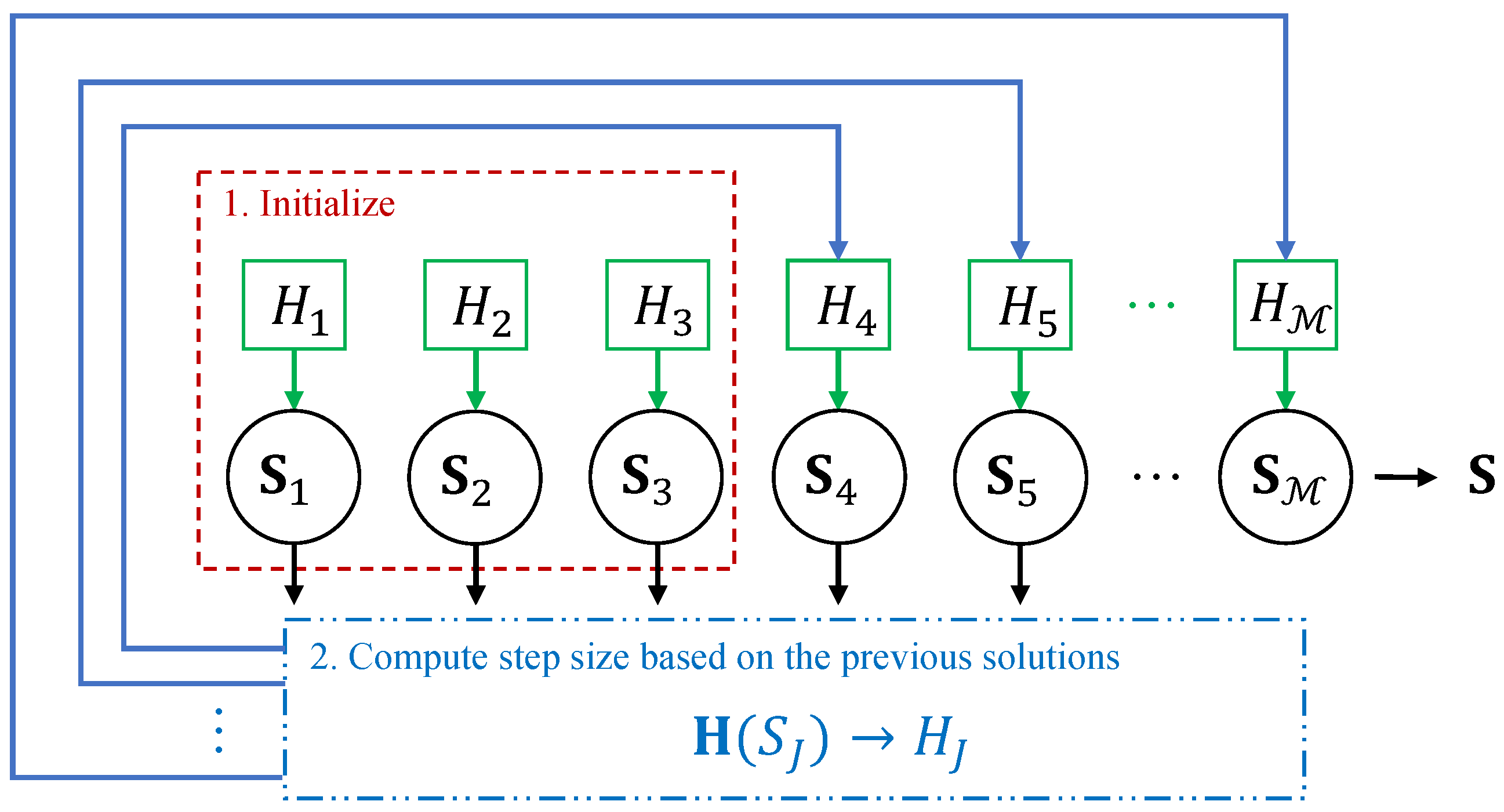Figure 1 visually demonstrates how the equations are solved using Strategy 1 in the AS-LMS. Figure 2 visualizes the logic of updating the step size, illustrating the evolution of the step size over three time steps as an example.

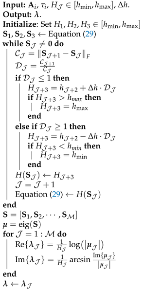
Strategy 1 is to update $H_{\mathcal{J}}$ based on the calculated solution at the current step with respect to the first step. This strategy is the most general one since it used the solution at the first numerical integration step as the reference. The final solution $\mathit{\lambda }$ can be accurately derived with fewer integration steps.

• Initialize the method: Start by choosing an initial step size $H_1,H_2,H_3$ from $H_{\mathcal{J}}\in [h_{\min },h_{\max }]$, where $h_{\min }$ and $h_{\max }$ are pre-defined values depending on the requirements and characteristics of the problem being solved. Define $\Delta h$ as the step size increment.
• Calculate the Frobenius norm of the matrices: Compute the change factor, ${\mathcal{C}}_{\mathcal{J}}$, of the calculated solution at the current time step. The following equation (33) is used to determine ${\mathcal{C}}_{\mathcal{J}}$ between the sub-matrices by using the Frobenius norm [27]. It can show how close the two matrices are to each other in terms of their individual elements.

  $${\mathcal{C}}_{\mathcal{J}}={\left|\right|{\mathbf{S}}_{\mathcal{J}+1}-{\mathbf{S}}_{\mathcal{J}}\left|\right|}_F\mathrm{for}\mathcal{J}=1,2,\cdots .$$

  (33)
• Calculate the changing rate of ${\mathcal{C}}_{\mathcal{J}}$: Compute the change of ${\mathcal{C}}_{\mathcal{J}}$, denoted as ${\mathcal{D}}_{\mathcal{J}}$, with respect to ${\mathcal{C}}_1$ as shown in (34). It shows the rate of change of the $S_{\mathcal{J}}$ matrices with respect to the first step change.

  $${\mathcal{D}}_{\mathcal{J}}={\displaystyle \frac{{\mathcal{C}}_{\mathcal{J}+1}}{{\mathcal{C}}_1}}.$$

  (34)
  Note that ${\mathcal{C}}_1$ would not be equal to zero, since ${\mathcal{C}}_1$ is a function of (29), where the coefficients ${\alpha }_j$ and ${\beta }_j$ depend on the steps of the AS-LMS method, and the coefficients are different, so that ${\mathbf{S}}_2$ ≠ ${\mathbf{S}}_1$.
• Step size control: Based on the computed ${\mathcal{D}}_{\mathcal{J}}$, adjust the step size for the next time step as shown in (35).

  $$H_{\mathcal{J}+3}=h_{\max }-\Delta h·{\mathcal{D}}_{\mathcal{J}}.$$

  (35)
  If the change factor is large, indicating rapid changes in the solution, the step size needs to be decreased to capture the behavior more accurately. Conversely, if the change factor is small, a larger step size needs to be used for efficiency.

Perform step 2 to step 4 in the stepping procedure of AS-LMS until the desired endpoint is reached, i.e., ${\mathbf{S}}_J=\mathbf{0}$. The above procedures are summarized in Algorithm 1.

Algorithm 1: Solving the Time-Delayed Microgrid System with AS-LMS Strategy 1

Strategy 2 is to update $H_{\mathcal{J}}$ based on the calculated solution at the current step with respect to its previous step. This strategy uses the solution from the previous numerical integration step as a reference, enabling the method to capture a broader range of eigenvalues, especially those distributed along the real axis. This approach enhances the capture of eigenvalues that may indicate stability changes in the system dynamics.

• Initialize the method: Start by choosing an initial step size $H_1,H_2,H_3$ from $H_{\mathcal{J}}\in [h_{\min },h_{\max }]$, where $h_{\min }$ and $h_{\max }$ are pre-defined values depending on the requirements and characteristics of the problem being solved. Define $\Delta h$ as the step size increment.
• Calculate the Frobenius norm of the matrices: Compute the change factor, ${\mathcal{C}}_{\mathcal{J}}$, of the calculated solution at the current time step.
• Calculate the changing rate of ${\mathcal{C}}_{\mathcal{J}}$: Compute the change of ${\mathcal{C}}_{\mathcal{J}}$, denoted as ${\mathcal{D}}_{\mathcal{J}}$, with respect to ${\mathcal{C}}_{\mathcal{J}}$ as shown in (36). It shows the rate of change of the $S_{\mathcal{J}}$ matrices with respect to the first step change.

  $${\mathcal{D}}_{\mathcal{J}}={\displaystyle \frac{{\mathcal{C}}_{\mathcal{J}+1}}{{\mathcal{C}}_J}}.$$

  (36)
  Note that ${\mathcal{C}}_{\mathcal{J}}$ would not be equal to zero, since ${\mathcal{C}}_{\mathcal{J}}$ is a function of (29), where the coefficients ${\alpha }_j$ and ${\beta }_j$ depend on the steps of the AS-LMS method, and the coefficients are different, so that ${\mathbf{S}}_{\mathcal{J}+1}$ ≠ ${\mathbf{S}}_{\mathcal{J}}$.
• Step size control: Based on the computed ${\mathcal{D}}_{\mathcal{J}}$, adjust the step size for the next time step as shown in (37).

  $$H_{\mathcal{J}+3}=\left\{\begin{array}{c}{h}_{\mathcal{J}+2}+\Delta h·{\mathcal{D}}_{\mathcal{J}},\mathrm{for}{\mathcal{D}}_{\mathcal{J}}\le 1,\hfill \\ h_{\mathcal{J}+2}-\Delta h·{\mathcal{D}}_{\mathcal{J}},\mathrm{for}{\mathcal{D}}_{\mathcal{J}}>1.\hfill \end{array}\right.$$

  (37)
  If the change factor is large, indicating rapid changes in the solution, the step size needs to be decreased to capture the behavior more accurately. Conversely, if the change factor is small, a larger step size needs to be used for efficiency.

Perform step 2 to step 4 in the stepping procedure of AS-LMS until the desired endpoint is reached, i.e., ${\mathbf{S}}_J=\mathbf{0}$. The above procedures are summarized in Algorithm 2.

Algorithm 2: Solving the Time-Delayed Microgrid System with AS-LMS Strategy 2

3.3. Performance of AS-LMS

As the system size increases, i.e., n in (7) and (8), the dimensionality of the resulting matrices, such as ${\mathbf{M}}_{\mathcal{I}}$ from (25), also increases correspondingly. Specifically, the matrix ${\mathbf{M}}_{\mathcal{I}}$ scales with the number of state variables. At the same time, when the step size h decreases, the computational complexity further intensifies. The size of the matrix $\mathbf{M}$ increases inversely with the step size, and as a result, the matrix dimension grows proportionally to ${\displaystyle \frac{1}{h}}$. This scaling highlights the dual impact of system size and step size on computational load: larger systems and smaller step sizes lead to significantly increased matrix dimensions, thereby imposing greater computational demands on stability analysis and simulation efforts.

Comparing to the general LMS, the AS-LMS has the following advantages. The advantages of the AS-LMS are shown in the cases studies.

3.3.1. Efficiency

Since the step size of the method is adaptively changed, the size of the results in (29) could be changed. Unlike $\mathcal{N}$ in (25) that is obtained from a fixed step size, the AS-LMS can dynamically update the step size during the calculation, so that $\mathcal{M}$ in (28) could reduced, i.e., $\mathcal{N}\ge \mathcal{M}$.

3.3.2. Accuracy

Meanwhile, even the step size changed, the accuracy of the resulting eigenvalues is maintaining at high level. Also, comparing to the case where the fixed h is large, $\mathcal{M}$ could be relatively increased, the accuracy of the resulting eigenvalues will also increase, i.e., inputting the resulting eigenvalues of (31) and (32) to (19) is no larger than inputting the resulting eigenvalues of (26) to (19). And more eigenvalues could be captured.

The AS-LMS method focuses on the analysis starting from the point where the state matrix $A_0$, the delayed state matrix $A_i$, and the delay $\tau$ are obtained. Once these inputs ($A_0$, $A_i$ and $\tau$) are provided, the method remains stable. As the number of state variables or the number of generator increases, the computational efficiency of the AS-LMS method becomes more advantageous compared to the LMS method. This is because the AS-LMS method can significantly reduce the size of the matrix $\mathbf{S}$ in (28), scaling as $n·g·(\mathcal{N}-\mathcal{M})$, where g represents the number of generators.

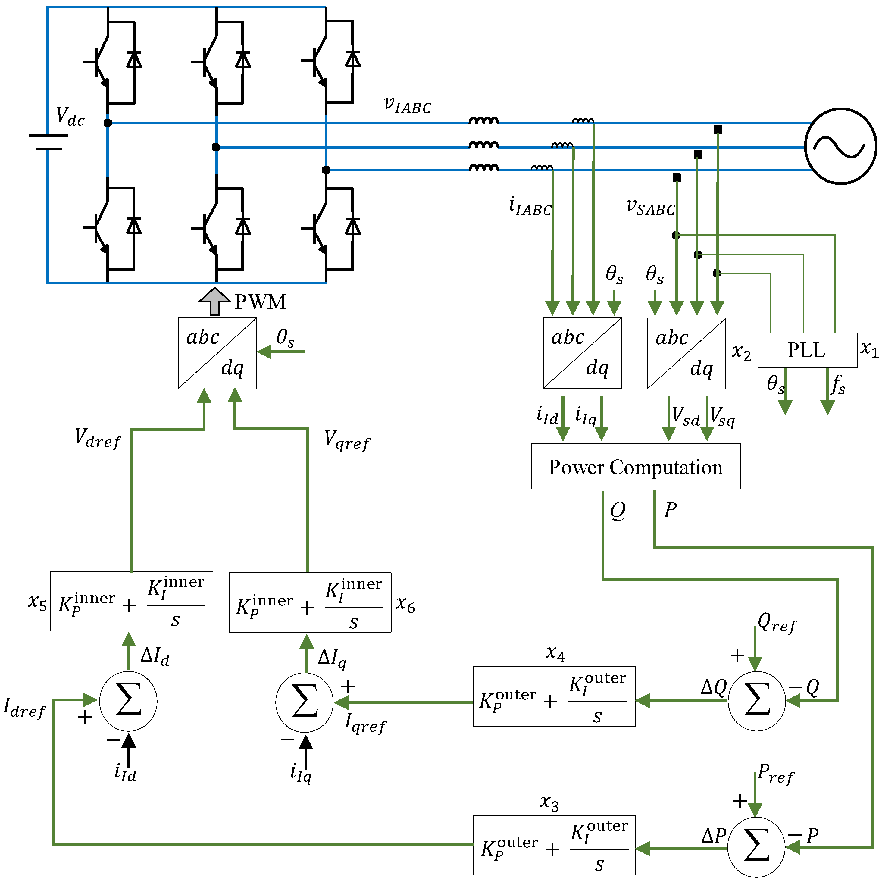
4. Case Study

In this section, we evaluate the performance of the proposed AS-LMS method on two standard testing systems: the IEEE 9-bus system and the IEEE 30-bus system. The parameters, including bus data, generator data and brance data for these test systems are obtained from [28]. The proposed algorithm was implemented and tested on a computer equipped with an Intel Core i5-9400F CPU, NVIDIA GeForce GTX 1660 Ti GPU, and 16 GB of memory. This computational setup was used to evaluate the execution time for various tests of the IEEE 30 bus testing case. The original generators in both IEEE testing cases are modified to converter-interfaced DER unit, i.e., solar photovoltaic systems. Six state variables for each generator are considered and shown in the Appendix. The microgrid operates in islanded mode. The system is designed to operate under normal conditions. The equilibrium point is reached and from this point, the state matrix $A_0$ and delayed state matrix $A_i$ are computed to analyze the system’s stability. Each testing system incorporates multiple time delays, which reflect the real-world communication delays in microgrids. Different step size strategies, including fixed and adaptive step sizes, are applied in the analysis. These strategies allow us to evaluate both the accuracy of the eigenvalue computations and the computational efficiency of the applied AS-LMS method. In the test cases, the Adams-Bashforth fourth-order method is used, i.e., $c=4$ in (21) and (27).

4.1. IEEE 9-Bus Test Case

There are three generators in the IEEE 9-bus test case, and each generator involved 6 state variables, so that the system has 18 state variables, i.e., $n=18$ from (7) and (8), leading to the system matrix ${\mathbf{A}}_0$ and the delayed state matrix ${\mathbf{A}}_i$ of size 18 by 18. The IEEE 9-bus system involved 6 time delays, i.e., one voltage signal delay and one current signal delay for each generator. The time delays in the system are chosen from the interval $\tau$ ∈ [$0.1$, $0.6$] s, representing communication and control delays commonly encountered in the system.

Figure 3 illustrates the eigenvalue distributions for four tests. The step sizes used of the four tests and the analysis of each case are introduced below.

• Fixed h = $0.03$: The eigenvalues computed using a small fixed step size of h = $0.03$ serve as a benchmark for eigenvalue accuracy, including the number of eigenvalues captured. The number of system matrix from (25) becomes 39, i.e., $\mathcal{N}$ = 39, which reflects the computational burden. The relatively small step size provides a more accurate approximation of the eigenvalues but incurs a higher computational cost due to the larger matrix size when compared to the following cases.
• Fixed h = $0.11$: Increasing the step size to h = $0.11$ reduces the computational burden, but the eigenvalue approximation deviates slightly from the reference values. The shift in eigenvalues is small. In this case, the number of system matrix from (25) becomes 15, i.e., $\mathcal{N}$ = 15, which significantly decreasing the computational effort compared to h = $0.03$. However, the precision of the approximation is lower and fewer eigenvalues are detected due to the larger step size.
• Adaptive $H_{\mathcal{J}}$∈ [$0.03$, $0.11$] strategy 1: The AS-LMS automatically increases or decreases the step size during the numerical integration using Algorithm 1, achieving a balance between accuracy and computational efficiency. The eigenvalues closely match those obtained with the smaller fixed step size h = $0.03$. The accuracy is maintained at a level comparable to that of the smaller fixed step size. The number of system matrix from (28) becomes 16, i.e., $\mathcal{M}$ = 16, the matrix size is significantly reduced, leading to more efficient computations. This shows that the AS-LMS effectively balances accuracy and efficiency by adjusting the step size.
• Adaptive $H_{\mathcal{J}}$∈ [$0.03$, $0.11$] strategy 2: The AS-LMS automatically increases or decreases the step size during the numerical integration using Algorithm 2, also achieving a balance between accuracy and computational efficiency. Different strategies can be useful for different testing cases and interested eigenvalues’ distributions. For example, in Figure 3, this strategy captures more eigenvalues with small real part comparing to all the other tests. The number of system matrix from (28) becomes 24, i.e., $\mathcal{M}$ = 24, the matrix size is reduced comparing to test 1, leading to more efficient computations. This shows that the AS-LMS can also effectively balances accuracy and efficiency by adjusting the step size.

Figure 4 illustrates the variation of the step size values of the 9 bus system tests at each numerical iteration during the implementation of AS-LMS. The step size is dynamically adjusted based on predefined criteria that aims to balance computational efficiency with the accuracy of the solution. As shown in the figure, the step size begins at an initial value of $h_{\min }=0.03$ and fluctuates within the allowable range up to $h_{\max }=0.11$. A key benefit of the AS-LMS is the reduction in the size of the system matrix $\mathbf{S}$ in (28) used in the LMS approximation, resulting in lower computational effort when solving for the system’s eigenvalues. The adaptivity of the step size allows to take larger steps in regions where the system solution is smoother and smaller steps when the solution exhibits rapid changes or when higher accuracy is required. This adaptive mechanism enhances both the efficiency and the precision of the eigenvalue estimation process.

The IEEE 9-bus testing example highlights the practical advantages of using AS-LMS in small signal stability analysis. The results demonstrate that the proposed AS-LMS method significantly reduces computational effort while maintaining a high level of accuracy in eigenvalue analysis. By dynamically adjusting the step size, the adaptive method optimizes the trade-off between precision and computational burden, making it highly suitable for real-time applications in microgrids where time delays and dynamic operating conditions play a critical role in system stability.

4.2. IEEE 30-Bus Test Case

To further demonstrate the efficacy of the AS-LMS method, we apply it to the IEEE 30-bus system, which consists of six generators, and each generator involved 6 state variables, so that the system has 36 state variables, i.e., $n=36$ from (7) and (8), leading to the system matrix ${\mathbf{A}}_0$ and the delayed state matrix ${\mathbf{A}}_i$ of size 36 by 36. The IEEE 30-bus system involved 12 time delays, i.e., two delays for each generator. The time delays in the system are chosen from the interval $\tau$∈ [$0.5$, $6.0$] seconds, simulating the communication and control delays encountered in large microgrids systems.

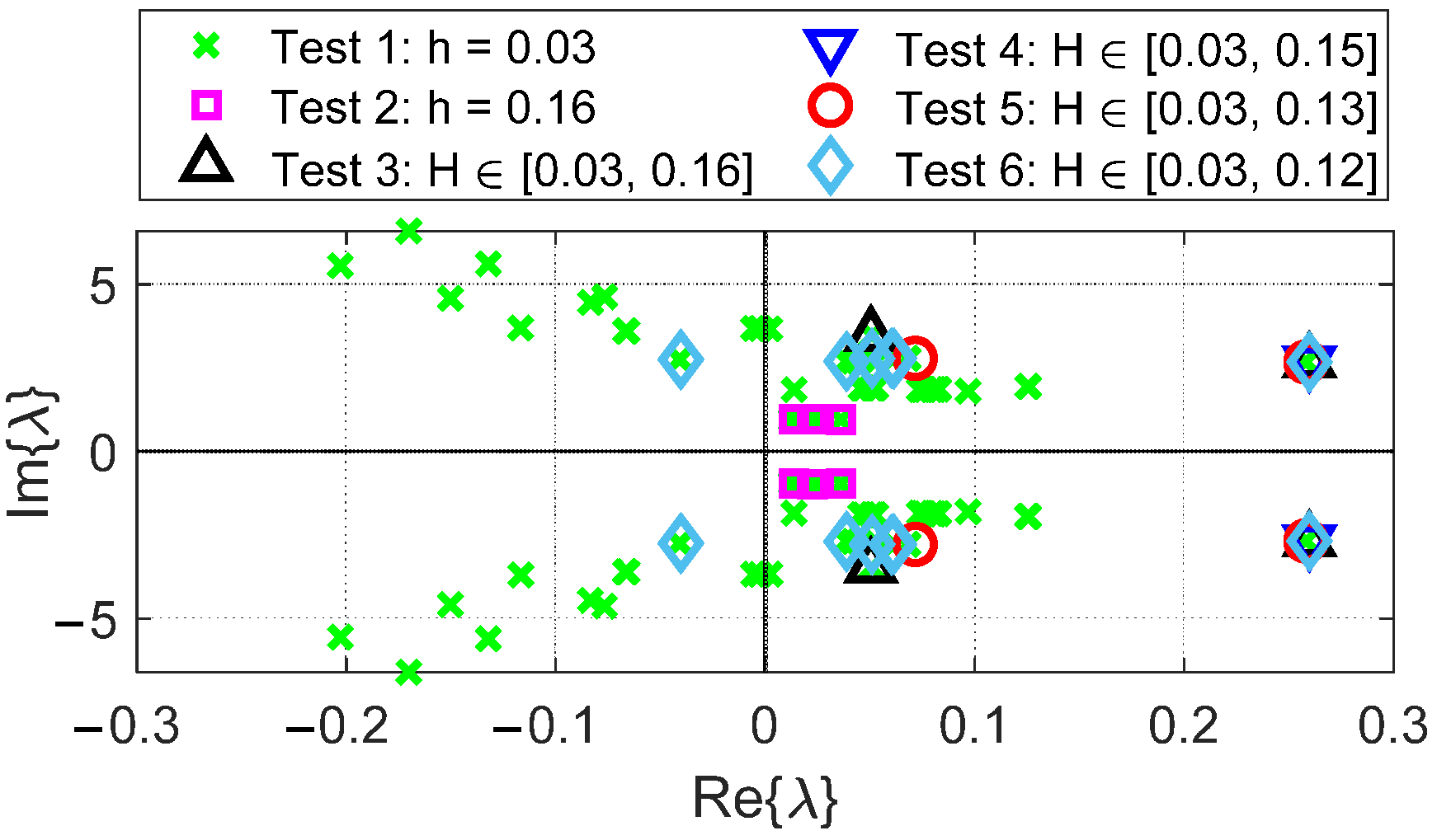
We conduct eight tests with different fixed step size, adaptive step size settings and adaptive strategies to assess how changing of the step size impacts the number of eigenvalues captured and the accuracy of the stability analysis. Each test is introduced below.

• Fixed $h=0.03$: The first test employs a fixed step size $h=0.03$, providing the highest accuracy by capturing most of the system’s eigenvalues, including the rightmost ones. The system matrix dimension is large, i.e., $\mathcal{N}$ = 39, reflecting the computationally intensive nature of this test, but it serves as a benchmark for captured eigenvalue accuracy.
• Fixed $h=0.16$: In the second test, a larger fixed step size of $h=0.16$ is used, which significantly reduces the computational burden, i.e., $\mathcal{N}$ = 12. However, this comes at the expense of accuracy, as fewer eigenvalues are captured, and notably, the rightmost eigenvalues are not captured. The reduction in step size leads to a less precise stability assessment.
• Adaptive $H_{\mathcal{J}}\in [0.03,0.16]$: The third test introduces an adaptive step size with the range $H_{\mathcal{J}}\in [0.03,0.16]$. While more eigenvalues are captured compared to Test 2, the method still fails to capture the rightmost eigenvalues. This highlights that the larger maximum step size ($h=0.16$) still limits the precision of eigenvalue computations.
• Adaptive $H_{\mathcal{J}}\in [0.03,0.15]$: In Test 4, the maximum step size is reduced to $h_{\max }=0.15$, leading to improved numbers of eigenvalue that can be captured. More eigenvalues are found compared to Test 3, including the rightmost ones. However, some important non-rightmost eigenvalues are still missing, indicating that further refinement of the maximum step size is necessary for comprehensive stability analysis.
• Adaptive $H_{\mathcal{J}}\in [0.03,0.13]$: In Test 5, the step size range is further reduced to $H_{\mathcal{J}}\in [0.03,0.13]$, resulting in the captures of more eigenvalues than in Test 4. The number of system matrix from (28) becomes 13, i.e., $\mathcal{M}$ = 13. The accuracy of the captured eigenvalue improves.
• Adaptive $H_{\mathcal{J}}\in [0.03,0.12]$ with strategy 1: Test 6 implements an adaptive step size with a range of $H_{\mathcal{J}}\in [0.03,0.12]$. The number of system matrix from (28) becomes 14, i.e., $\mathcal{M}$ = 14. This test provides the most comprehensive eigenvalue captures after Test 1, striking a good balance between computational efficiency and accuracy. The rightmost eigenvalues are captured, and the number of non-rightmost eigenvalues captured is higher than in the previous tests.
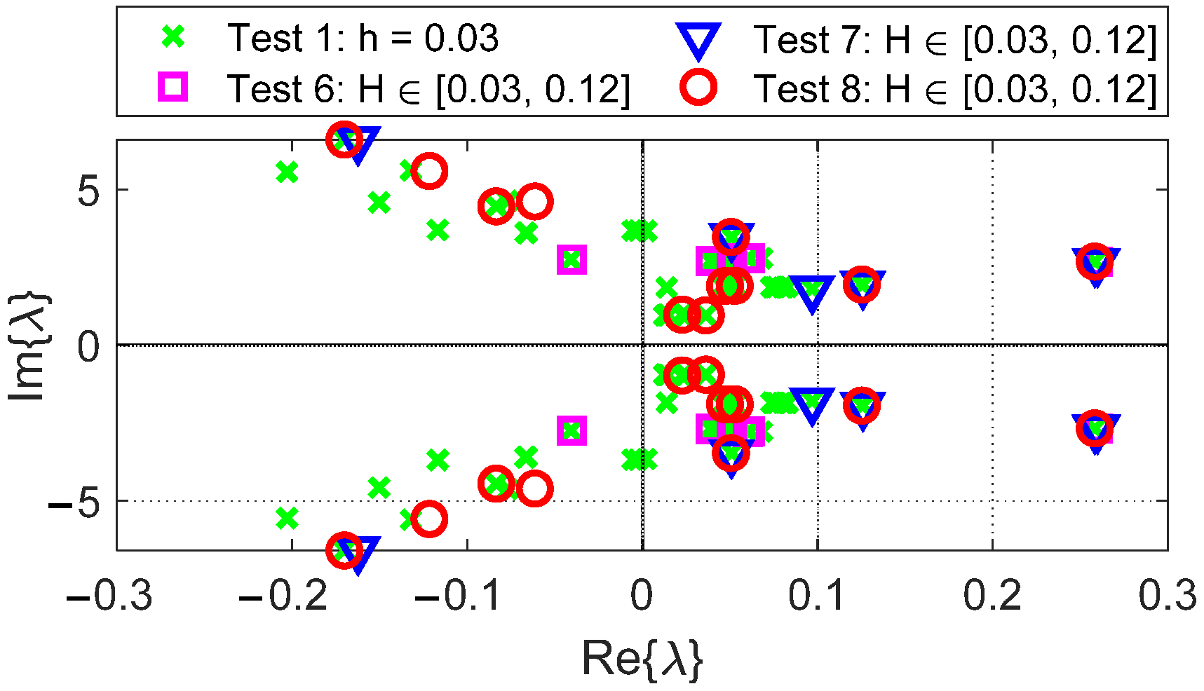
• Adaptive $H_{\mathcal{J}}\in [0.03,0.12]$ with strategy 2: Test 7 implements an adaptive step size with a range of $H_{\mathcal{J}}\in [0.03,0.12]$ with strategy 2. This test initialize the first three numerical steps to $h_{\min }$. The number of system matrix from (28) becomes 32, i.e., $\mathcal{M}$ = 32. This test provides another comprehensive eigenvalue captures after Test 1. However, this strategy used more numerical integration steps than that of Test 6.
• Adaptive $H_{\mathcal{J}}\in [0.03,0.12]$ with strategy 2: Test 8 implements an adaptive step size with a range of $H\in [0.03,0.12]$ with strategy 2. The number of system matrix from (28) becomes 30, i.e., $\mathcal{M}$ = 30. This test starts from $h_{\max }$ provides another comprehensive eigenvalue captures after Test 1. This strategy used less numerical integration steps than that of Test 7.

Figure 5 shows the eigenvalue distributions for the first six tests. Figure 6 shows the eigenvalue distributions of test 1, test 6 and two tests with different settings and strategies, i.e., test 7 and 8. As the maximum step size is reduced, the number of captured eigenvalues increases, particularly those that are critical for assessing system stability (i.e., the rightmost eigenvalues). Test 1 remains the most accurate, capturing the rightmost eigenvalues, while Test 6 offers a practical compromise between accuracy and computational effort.

Figure 7 demonstrates the variation in step size values for the four tests with adaptive strategy 1 conducted on the IEEE 30-bus system. The figure illustrates the dynamic adjustment of the step size $H_{\mathcal{J}}$, where each curve corresponds to one of the four tests with different maximum allowable step sizes: $h_{\max }=0.16$, $h_{\max }=0.15$, $h_{\max }=0.13$, and $h_{\max }=0.12$, respectively. For smaller $h_{\max }$, it allows for a more precise approximation of eigenvalues. As $h_{\max }$ increases, the method may lose precision in capturing these sensitive eigenvalues, though it can reduce the computational burden by using fewer steps. 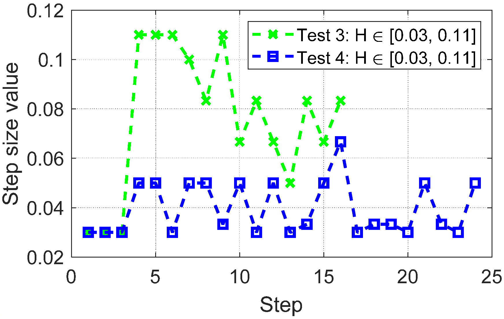The step size starts from a minimum value of $h_{\min }=0.03$ and adapts based on the local system dynamics. Each curve exhibits fluctuations that reflect the balance between computational efficiency and the accuracy required for capturing eigenvalue distributions. Specifically, smaller step sizes are applied when the system’s behavior becomes more complex, while larger steps are used in smoother regions. The adaptivity in step size, evident from the figure, highlights the role of the maximum step size setting in improving the captures of important eigenvalues, particularly the rightmost ones. As the maximum step size decreases, the algorithm becomes capable of identifying a greater number of eigenvalues with higher accuracy, though at the cost of increased computational time.

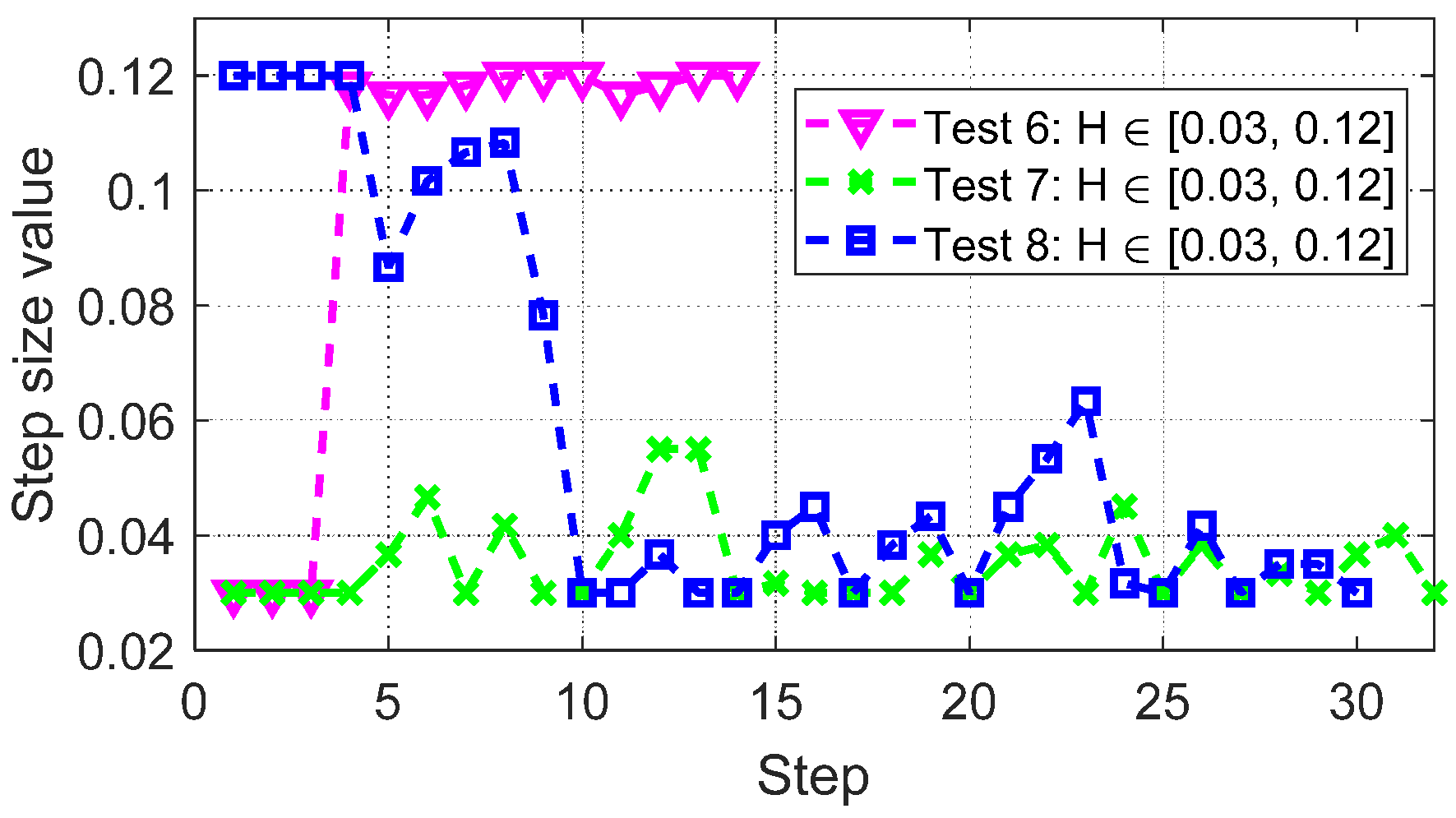
Figure 8 shows the step size changes with different updating strategies and settings. The resulting size of the problem are quite different. The dimensions of strategy 2 is relatively larger than that of strategy 1 in this particular example.

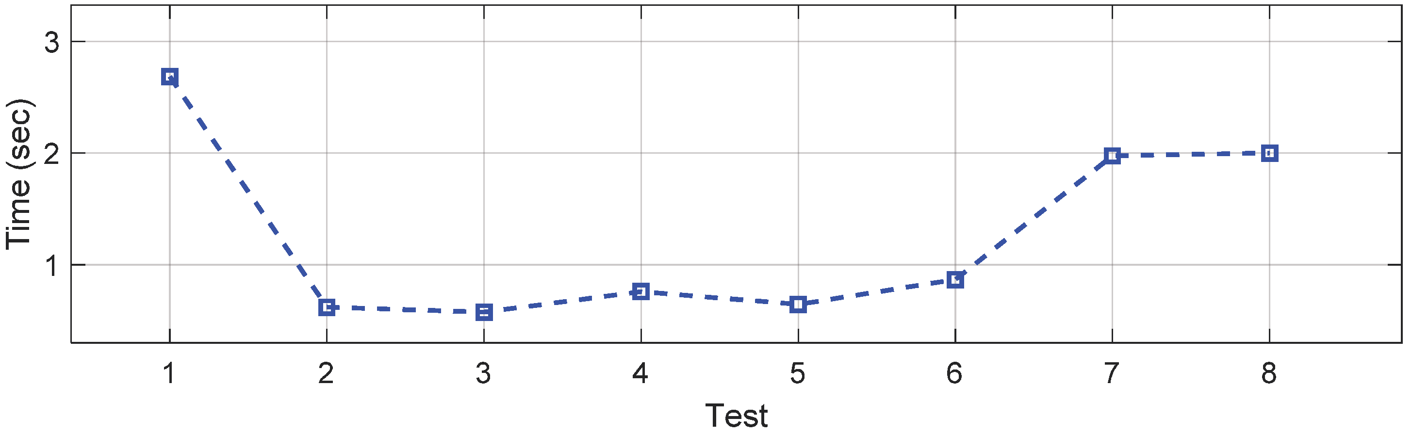
Figure 9 illustrates the execution time for each test that is conducted on the IEEE 30-bus testing system. Test 1 has the longest execution time, which is expected given its smallest step size. The results of Tests 2, 3, and 4 are not discussed in detail because their step-size selection does not yield optimal performance due to inappropriate settings. These tests are included primarily for demonstration purposes, illustrating the potential consequences of selecting inappropriate step size settings. Test 5, 6, 7, and 8 demonstrate significantly decreased execution times compared to Test 1. The execution time for Tests 5, 6, and 7 increases as the problem size increases, i.e., as $\mathcal{M}$ becomes larger. Tests 7 and 8 exhibit similar execution times, as their only difference lies in the initial step size. Tests employed with the AS-LMS demonstrate a significant advantage in saving computational time while still successfully capturing the rightmost eigenvalues.

Equation (19) can be used to verify whether an eigenvalue represents a true solution, with the final results expected to approach zero as closely as possible. In the IEEE 30 bus testing case, when the resulting rightmost eigenvalues $\lambda$ are substituted into (19), the results are shown in

Table 1. The rightmost eigenvalue accuracy for the IEEE 30 bus testing case.

Test	Eigenvalue Accuracy
Test 1	$-8.95783126227976\times {10}^{-14}+3.23966325574453\times {10}^{-15}i$
Test 5	$-1.21288725494212\times {10}^{-14}-6.67934813906719\times {10}^{-15}i$
Test 6	$4.24566409555860\times {10}^{-13}+3.80009861063769\times {10}^{-12}i$
Test 7	$-7.23308832301429\times {10}^{-15}+4.61940636957513\times {10}^{-15}i$
Test 8	$-8.59638744258942\times {10}^{-15}-6.89050333856057\times {10}^{-15}i$

.

All of these values are sufficiently close to zero, demonstrating that the AS-LMS method achieves good accuracy during implementation.

The IEEE 30-bus test case highlights the effectiveness of the AS-LMS method in tracking the rightmost eigenvalues, which are essential for assessing system stability. By focusing on the rightmost eigenvalues, we can quickly determine the stability of the system with reduced computational effort. The AS-LMS efficiently balances accuracy and computational burden by dynamically adjusting the time step based on system dynamics. This makes the method particularly well-suited for larger, more complex power systems like the IEEE 30-bus system, where time delays and dynamic operating conditions can significantly impact stability.

5. Conclusions

The paper began with a detailed discussion of the importance of small signal stability analysis in power systems, particularly due to the increasing penetration of DERs and the dynamic nature of power flow in such systems. The inherent time delays in their communication and control systems can degrade their small signal stability, affecting reliable operation. This paper presents an Adaptive Step Size Linear Multistep Method (AS-LMS), for analyzing small signal stability of the system in the presence of time delays. This method balances accuracy and computational efficiency by reducing the size of the system matrix without compromising the precision of eigenvalue computations. The AS-LMS was shown to outperform fixed step size approaches, particularly in terms of reducing computational effort while maintaining accurate stability assessments. Numerical examples, including tests on the IEEE 9-bus and 30-bus systems, confirmed the accuracy and the efficiency of the proposed method. For both systems, the AS-LMS was able to accurately track the rightmost eigenvalues, which are critical for stability analysis, while significantly reducing the computational burden. In particular, the AS-LMS demonstrated comparable accuracy to the smaller fixed step size cases, but with far less computational overhead. The AS-LMS method offers a promising approach for analyzing the small signal stability of microgrids with time delays. Its ability to dynamically adjust the step size makes it particularly suitable for large and complex power systems where time delays can significantly impact stability. However, a limitation arises in that some non-rightmost eigenvalues may not be effectively captured. For scenarios where identifying as many eigenvalues as possible is critical, the AS-LMS method would benefit from further development of adaptive strategies. These strategies could, for instance, focus on optimizing the coefficients and dynamically adjusting the step size functions to enhance the method’s capability to capture a broader spectrum of eigenvalues. Advancing such adaptive techniques represents a significant direction for future research to improve the applicability and robustness of the AS-LMS method. Also, the future work could further investigate the impact of varying types of time delays on stability.