Multithreaded and GPU-Based Implementations of a Modified Particle Swarm Optimization Algorithm with Application to Solving Large-Scale Systems of Nonlinear Equations

Abstract

This paper presents a novel Graphics Processing Unit (GPU) accelerated implementation of a modified Particle Swarm Optimization (PSO) algorithm specifically designed to solve large-scale Systems of Nonlinear Equations (SNEs). The proposed GPU-based parallel version of the PSO algorithm uses the inherent parallelism of modern hardware architectures. Its performance is compared against both sequential and multithreaded Central Processing Unit (CPU) implementations. The primary objective is to evaluate the efficiency and scalability of PSO across different hardware platforms with a focus on solving large-scale SNEs involving thousands of equations and variables. The GPU-parallelized and multithreaded versions of the algorithm were implemented in the Julia programming language. Performance analyses were conducted on an NVIDIA A100 GPU and an AMD EPYC 7643 CPU. The tests utilized a set of challenging, scalable SNEs with dimensions ranging from 1000 to 5000. Results demonstrate that the GPU accelerated modified PSO substantially outperforms its CPU counterparts, achieving substantial speedups and consistently surpassing the highly optimized multithreaded CPU implementation in terms of computation time and scalability as the problem size increases. Therefore, this work evaluates the trade-offs between different hardware platforms and underscores the potential of GPU-based parallelism for accelerating SNE solvers.

1. Introduction

Particle Swarm Optimization (PSO) [1] is among the most prominent metaheuristic algorithms in the literature [2] alongside genetic algorithms [3], differential evolution [4,5], and ant colony optimization [6]. PSO has garnered substantial attention across various research fields due to its simplicity, accelerated convergence, and robust effectiveness in optimizing a wide range of real-world problems [7]. Consequently, numerous PSO variants have been proposed to enhance its optimization performance and address the limitations of the standard PSO in specific contexts. An example of these variants is the algorithm proposed by Jaberipour et al. [8], which modifies the PSO approach to tackle Systems of Nonlinear Equations (SNEs) more efficiently.

Addressing these SNEs is one of the most complex challenges in numerical analysis, particularly for large-scale systems. These difficulties stem from the inherent complexity of nonlinear relationships, potential non-convexities, and the significant computational cost required to obtain accurate solutions. Furthermore, in large-scale SNEs, increased dimensionality imposes a substantial burden, resulting in a notable rise in computational cost.

Iterative numerical techniques, such as Newton’s method and its variants, are among the most widely used solvers for SNEs [9]. However, the effectiveness of these methods can be considerably dependent on the initial approximation of the solution [10,11], which can lead to suboptimal solutions, nonconvergence [12], or an estimation process that is excessively time consuming [13]. Additionally, as the dimensionality of SNEs increases, the computational burden grows rapidly, considerably raising both time and resource requirements. In large-scale SNEs, this dimensional growth amplifies the challenge of finding optimal or near-optimal solutions within a feasible timeframe. Consequently, the development of more efficient computational approaches is crucial and encompasses the use of both enhanced solvers and more effective implementations.

Metaheuristic algorithms, such as PSO, have gained increasing attention for their effectiveness in addressing complex numerical challenges, including their successful application to solving SNEs (see, e.g., [14,15,16,17,18,19]). Furthermore, such approaches offer several advantages over traditional methods. Metaheuristic algorithms can efficiently handle large, high-dimensional problems, yield near-optimal solutions in a timely manner, and do not rely on accurate initial approximations for success. Instead, they perform global searches using randomly generated starting points. While metaheuristic algorithms cannot guarantee exact solutions, they are typically less computationally demanding, making them more efficient solvers.

However, using these approaches alone is not enough to considerably reduce the time needed to solve large-scale problems with thousands of equations and variables. To achieve substantial reductions in computational time, more efficient implementation strategies are required, particularly through the use of high-performance computing techniques, such as heterogeneous architectures. This combination enables the study of more complex problems that would otherwise be impractical with traditional approaches.

This work proposes a novel enhanced Graphics Processing Unit (GPU)-based parallelization of a variant of the PSO algorithm optimized for solving SNEs, called PPSO [8], which is capable of handling large-scale problems effectively. The proposed GPU parallelization methodology accelerates computation while preserving the core operating mechanisms of the standard approach. In addition, a performance-optimized multithreaded version of the algorithm is proposed, which also retains the fundamental operating principles of the standard algorithm. This alignment ensures that both the GPU-based and multithreaded implementations maintain the theoretical consistency of the original, including its convergence properties. As a result, the comparison of computation times across the different implementations becomes more robust and meaningful, as the underlying mechanisms remain unchanged, enabling a fairer evaluation of performance improvements in efficiency, scalability, and execution speed. The effectiveness of these approaches is assessed by comparing the GPU parallel implementation of the PSO variant with the sequential and multithreaded versions, evaluating overall computation time and speedup across different hardware architectures and problem sizes (i.e., the number of equations and variables in each system).

To solve SNEs using metaheuristic algorithms, they must first be transformed into an optimization problem. Consider an SNE consisting of n nonlinear equations with n unknowns, represented in its general vector form as $f(\mathit{x})=\mathbf{0}$, where the equations that make up the system are expressed as $f_i(x_1,\dots ,x_n)=0,i=1,\dots ,n$. A common approach to solving such a system involves reformulating the SNE into an n-dimensional nonlinear minimization problem. In this paper, the objective function is defined as ${\sum }_{i=1}^n\left|f_i(x_1,\dots ,x_n)\right|$, which represents the sum of the absolute values of the residuals. By minimizing this objective function, the goal is to find a solution where the residuals, and thus the components of $f(\mathit{x})$, are driven as close to zero as possible. This approach facilitates the use of optimization techniques to solve SNEs, providing a systematic framework for addressing such systems in diverse contexts.

This article is organized as follows: Section 2.3 provides a review of previous research and methodologies related to PSO and its applications in optimization, focusing particularly on advancements in parallel and multithreaded implementations. Section 3 provides a detailed overview of the PSO algorithm and the proposed multithreaded and parallel approaches. The principles and mechanics of the PSO algorithm, including its variant for solving SNEs, are discussed in Section 2.1, while the proposed multithreaded and GPU-based parallelizations are presented in detail in Section 3.2 and Section 3.3, respectively. Section 4 outlines the computational experiments conducted to evaluate the performance of the different implementations, detailing the specifications of the experimental setup (Section 4.2) and the characteristics of the selected test problems (Section 4.2). Section 5 presents the results of the computational experiments and provides a detailed discussion of the findings. Finally, Section 6 summarizes the key findings of the article, including potential areas for further research.

2. Background and Related Work

PSO is a well-established optimization algorithm known for its simplicity and efficiency in solving complex problems. This section provides an overview of the PSO algorithm and explores its application to SNEs through a variant known as PPSO. Additionally, the related work in the field is reviewed with a focus on parallelization approaches developed to enhance performance.

2.1. Particle Swarm Optimization Algorithm

The PSO algorithm is an optimization technique inspired by natural social behaviors, such as bird flocking or fish schooling. Introduced in 1995 by James Kennedy and Russell Eberhart [1], PSO is a computational method that solves optimization problems by mimicking the collective behavior of particles moving through a search space. The algorithm exploits the collective dynamics of the swarm to navigate the solution space, converging toward the optimal solution. Through the exchange of information derived from their individual experiences, the particles can enable the swarm to effectively identify global optima even in complex, high-dimensional problem spaces.

In PSO, each solution is represented by a particle, which has both a position and a velocity. The position corresponds to a candidate solution, while the velocity dictates how the particle moves through the solution space. As particles navigate through the search space, they explore potential solutions, adjusting their positions based on their individual experiences as well as the collective knowledge of the swarm.

The velocity of each particle is updated based on two primary influences. The cognitive component $c_1$ drives the particle toward its own best-known position (referred to as its personal best or $pBest$), and the social component $c_2$, which attracts the particle to the best position found by any particle in the swarm (the global best $gBest$).

Given a design variable index $v\in \{1,\dots ,numVars\}$, where $numVars$ is the number of decision variables, a population index $p\in \{1,\dots ,popSize\}$, where $popSize$ is the population size, and an iteration index $i\in \{1,\dots ,maxIters\}$, where $maxIters$ is the maximum number of iterations, the velocity update $V_{p,v}^{i+1}$ is determined using the following equation:

$$V_{p,v}^{i+1}=\omega V_{p,v}^i+c_1{r}_{1,v}^i(pBes{t}_{p,v}^i-X_{p,v}^i)+c_2{r}_{2,v}^i(gBes{t}_v^i-X_{p,v}^i),$$

(1)

where $\omega$ is the inertia weight, $r_{1,v}^i$ and $r_{2,v}^i$ are random values between 0 and 1, and $X_{p,v}^i$ is the current position of particle p at dimension v.

The inertia weight parameter regulates the contribution of the previous velocity to the current velocity update, balancing the exploration and exploitation abilities of the swarm. A high inertia weight enables particles to explore the search space more freely, promoting a broader search and helping avoid becoming trapped in local optima. In contrast, a low inertia weight leads to smaller adjustments in the particles’ velocity, resulting in faster convergence to the best solution found.

After updating the velocity, the particle’s updated position $X_{p,v}^{i+1}$ is obtained in the following way:

$$X_{p,v}^{i+1}=X_{p,v}^i+V_{p,v}^{i+1}.$$

(2)

The pseudocode outlining the main steps of the PSO algorithm is depicted in Algorithm 1, which includes the initialization phase, the main loop with updates to velocities, positions, personal bests, and global best along with the termination condition.

Algorithm 1 Pseudocode for standard PSO

1: /* Initialization */  2: Initialize $numVars$, $popSize$ and $maxIters$;  3: Initialize particles X and velocity vectors V;  4: Evaluate fitness values $f(X)$;  5: Initialize $pBest$;  6: Determine $gBest$;  7: $i\leftarrow 1$;  8: /* Main loop */  9: while $i\le maxIters$ do 10:   for $p\leftarrow 1,popSize$ do 11:     for $v\leftarrow 1,numVars$ do 12:       Update velocity $V_{p,v}^i$ using Equation (1); 13:       Apply velocity constraints $V_{p,v}^i$; 14:       Update position $X_{p,v}^i$ using Equation (2); 15:       Apply boundary constraints $X_{p,v}^i$; 16:     end for 17:     Evaluate fitness value $f(X_{p,v}^i)$; 18:     if $f(X_{p,v}^i)<f(pBes{t}_{p,v}^i)$ then           ▹ Update $pBest$ 19:       $pBes{t}_{p,v}^i\leftarrow X_{p,v}^i$; 20:     end if 21:   end for 22:   for $p\leftarrow 1,popSize$ do 23:     if $f(pBes{t}_{p,v}^i)<f(gBes{t}_v^i)$ then          ▹ Update $gBest$ 24:       $gBes{t}_v^i\leftarrow pBes{t}_{p,v}^i$; 25:     end if 26:   end for 27:   $i\leftarrow i+1$; 28: end while 29: Output the best solution found and terminate.

The velocity and boundary constraint actions, as indicated in lines 13 and 15 of Algorithm 1, are implemented to control the behavior of particles during the optimization process by constraining their positions to specified ranges. These functions ensure effective exploration of the search space by preventing particles from moving too quickly, which might cause them to overshoot optimal solutions, or from exceeding the defined search domain.

2.2. PSO for Solving SNEs

Jaberipour et al. [8] proposed a modified version of the PSO algorithm aimed at enhancing its effectiveness in solving complex SNEs. This new variant, referred to as PPSO, improves upon the update mechanism of the original PSO to address some of its limitations, such as rapid convergence during the initial search phase followed by slower progress and an increased risk of getting trapped in local minima. The authors successfully compared the results obtained using the PPSO algorithm with those produced by standard SNE solvers, including the Newton method, and demonstrated the efficiency of PPSO.

In PPSO, the cognitive and social components are more dynamic, introducing greater randomness and flexibility compared to the fixed scaling factors in the original PSO. These modifications aim to help the particles escape local minima and improve the overall convergence by allowing particles to receive more flexible influence from $pBest$ and $gBest$.

The velocity update equation for PPSO is as follows:

$$V_{p,v}^{i+1}=(2r_{1,v}^i-0.5)V_{p,v}^i+(2r_{2,v}^i-0.5)(pBes{t}_{p,v}^i-X_{p,v}^i)+(2r_{3,v}^i-0.5)(gBes{t}_v^i-X_{p,v}^i),$$

(3)

where $r_{1,v}^i$, $r_{2,v}^i$, and $r_{3,v}^i$ are random values between 0 and 1.

To enhance the adaptability of the PPSO algorithm and achieve a more dynamic balance between exploration and exploitation during the search, the inertia weight is updated dynamically (instead of being constant or linearly decreasing), as indicated by the following equation:

$${\omega }^{i+1}=(2r_{4,v}^i-0.5)(gBes{t}_v^i-pBes{t}_{p,v}^i)+(2r_{5,v}^i-0.5)(gBes{t}_v^i-X_{p,v}^i),$$

(4)

where $r_{4,v}^i$ and $r_{5,v}^i$ are random values between 0 and 1.

Rather than relying solely on the current position of the particle and its updated velocity, the position update in PPSO is modified by incorporating additional random factors in a more complex formula. This formula includes a modification factor applied to both the velocity and the inertia weight (which was moved from the velocity equation in the original PSO), as

$$X_p^{i+1}=pBes{t}_{p,v}^i+(2r_{6,v}^i-0.5)V_p^{t+1}+(2r_{7,v}^i-0.5){\omega }^{i+1},$$

(5)

where $r_{6,v}^i$ and $r_{7,v}^i$ represent random values uniformly distributed between 0 and 1.

One of the novel aspects of PPSO is the handling of the worst $pBest$ position, which is referred to as $pWorst$. In this approach, a randomly chosen component l of $pWorst$ is updated using the following equation:

$$pWors{t}_l^{new}=pWors{t}_l^i+(2r_{8,v}^i-0.5){\displaystyle \frac{f(pWors{t}^i+e_lϵ)-f(pWors{t}^i-e_lϵ)}{2ϵ(U{B}_l-L{B}_l)}},$$

(6)

where $r_{8,v}^i$ is a random value between 0 and 1, $e_l$ is the l-th unit vector, $ϵ$ is set to ${10}^{-8}$, $U{B}_l$ is the upper bound of the l-th variable, and $L{B}_l$ is the lower bound.

The pseudocode outlining the step-by-step procedure of the PPSO algorithm is presented in Algorithm 2.

Algorithm 2 Pseudocode for PPSO

1: /* Initialization */  2: Initialize $numVars$, $popSize$, and $maxIters$;  3: Initialize particles X and velocity vectors V;  4: Evaluate fitness values $f(X)$;  5: Initialize $pBest$;  6: Determine $gBest$;  7: $i\leftarrow 1$;  8: /* Main loop */  9: while $i\le maxIters$ do 10:   for $p\leftarrow 1,popSize$ do 11:     for $v\leftarrow 1,numVars$ do 12:       Update velocity $V_{p,v}^i$ using Equation (3); 13:       Apply velocity constraints $V_{p,v}^i$; 14:       Update position $X_{p,v}^i$ using Equation (5); 15:       Apply boundary constraints $X_{p,v}^i$; 16:     end for 17:     Evaluate fitness value $f(X_{p,v}^i)$; 18:     if $f(X_{p,v}^i)<f(pBes{t}_{p,v}^i)$ then           ▹ Update $pBest$ 19:       $pBes{t}_{p,v}^i\leftarrow X_{p,v}^i$; 20:     end if 21:   end for 22:   for $p\leftarrow 1,popSize$ do 23:     if $f(pBes{t}_{p,v}^i)<f(gBes{t}_v^i)$ then          ▹ Update $gBest$ 24:       $gBes{t}_v^i\leftarrow pBes{t}_{p,v}^i$; 25:     end if 26:     if $f(pBes{t}_{p,v}^i)>f(pWors{t}^i)$ then        ▹ Determine $pWorst$ 27:       $pWors{t}^i\leftarrow pBes{t}_{p,v}^i$; 28:     end if 29:   end for 30:   $l\leftarrow rand(1,numVars)$;        ▹ Select random component of $pWorst$ 31:   Determine $pWors{t}_l^{new}$ using Equation (6); 32:   Apply boundary constraints $pWors{t}_l^{new}$; 33:   if $f(pWors{t}^{new})<f(pWors{t}^i)$ then        ▹ Update $pWorst$ 34:     $pWors{t}^i\leftarrow pWors{t}^{new}$; 35:     if $f(pWors{t}^i)<f(gBes{t}_v^i)$ then         ▹ Update $gBest$ 36:       $gBes{t}_v^i\leftarrow pWors{t}^i$; 37:     end if 38:   end if 39:   $i\leftarrow i+1$; 40: end while 41: Output the best solution found and terminate.

2.3. Related Work

According to Lalwani et al. [20], aside from distributed parallel computing, most efforts to parallelize PSO and its variants primarily focus on leveraging GPUs, which is followed by CPU-based parallelization. These parallelization techniques aim to accelerate the optimization process by distributing computational tasks across multiple processing units, thereby reducing execution times, especially for large-scale or computationally intensive problems.

Hussain and Fujimoto [21] proposed a GPU-based parallel Multi-Objective Particle Swarm Optimization (MOPSO) approach for large swarms and high-dimensional problems, using a master–slave model. In this GPU MOPSO implementation, the CPU serves as the master, controlling the GPU threads, which function as the slaves, distributing the computational workload across multiple processing units to accelerate the evaluation of particles. The GPU computation employs multiple kernels, each handling different aspects of the optimization process in parallel. The paper compares the GPU-based algorithm to a sequential implementation, which was also optimized for large swarms and high-dimensional problems. The GPU-based MOPSO achieved a maximum speedup of 157$\times$ over the sequential algorithm at a problem dimension of 1024 with 40,000 particles and 1500 iterations. The algorithms were implemented in CUDA using C++, and tests were performed using a 4-core Intel Xeon E3-1220 v5 CPU with 16 GB of RAM and an NVIDIA Titan V GPU with 5120 cores and 12 GB of VRAM.

cuPSO [22] is a queue-based GPU parallelization for PSO algorithms that aims to address the reduction-based method, which is commonly used for handling data aggregation and parallel updates in PSO. The reduction strategy involves efficiently aggregating or reducing data across many threads in a GPU. In cuPSO, this strategy is optimized using a queue algorithm with atomic locks, which, according to the authors, is 2.2$\times$ faster compared to the parallel reduction-based method. The algorithms used CUDA and were programmed in C++, and tests were conducted using double-precision floating-point operations in low and high-dimensional search spaces of 1 dimension and 120 dimensions, respectively. Using an Intel Xeon CPU E3-1275 v5 and an NVIDIA GTX 1080 Ti, the GPU-based algorithm achieved a maximum improvement ratio of 217.78$\times$ at a problem dimension of 120 with 131,072 particles and 800 iterations.

A GPU-accelerated version of the Improved Comprehensive Learning Particle Swarm Optimization (ICL-PSO) algorithm was proposed by Wang et al. [23] to identify heat transfer coefficients in continuous casting. The implementation uses a two-layer parallel processing structure, consisting of the parallel heat transfer model and the parallel ICL-PSO, to reduce computing time. However, the GPU parallelization relies on multiple data transfers between the CPU and GPU, which is not an efficient approach. As a result, the maximum achieved speedup was 37$\times$, using test parameters that included 60 iterations, 36 particles, and $2.884\times {10}^6$ mesh points. This CUDA-based algorithm was implemented in C++, and the performance evaluation used an Intel Core i7-12700F CPU with 8 GB of RAM and an NVIDIA Tesla V100 with 32 GB VRAM.

A new implementation to reduce the execution time of PSO using OpenCL was proposed by Chraibi et al. [24]. OpenCL is a data-parallel, high-performance framework designed for heterogeneous computing, supporting multiple devices such as GPUs, CPUs, and Field Programmable Gate Arrays (FPGAs). This makes OpenCL both a cross-platform and hardware-agnostic framework. The implementation relies on kernel functions to execute code, similarly to CUDA, and the algorithm written in Java parallelizes only the particle updates and fitness calculations. Tests were performed using two CPUs, the Intel Core i7-6500U and Intel Xeon E5-2603 v4, and two GPUs, the Intel HD Graphics 520 and GeForce 920M. The authors report a maximum speedup of 9$\times$ for the parallel algorithm over the sequential version, which was achieved with the Core i7-6500U CPU using the Sphere function at a dimension of 100,000 with 100 iterations and a swarm size of 100.

Kumar et al. [25] proposed a parallel implementation of PSO to enhance performance on general-purpose computer architectures, as many researchers lack access to high-performance computing resources. The parallel tasks in this implementation include particle initialization, particle updates, fitness evaluation, and $pBest$ updates, diverging from the conventional approach of only parallelizing fitness function evaluations. Tests were conducted using several optimization benchmark functions and multiple combinations of parameters, including population size (40, 80, and 100), maximum iterations (10 and 30), and problem dimensionality (ranging from 10 to 4000). The algorithm was programmed using MATLAB, and performance evaluation was carried out using three distinct CPUs: the Intel Core i3 6006U, Intel Core i5-8500, and Intel Xeon E5-2650 v3. The maximum overall speedup achieved was 5.23$\times$ using the Intel Xeon E5-2650 v3 with a population size of 80, 10 iterations and a dimensionality of 4000.

A multi-core parallel PSO (MPPSO) algorithm [26] was developed to improve computational efficiency for the long-term optimal operation of hydropower systems. In this approach, a fork/join framework utilizing a divide-and-conquer strategy is used to allocate multiple populations across different CPU cores for parallel processing. This setup introduces a slight modification to the traditional PSO operating principle, as the search space is divided into several sub-populations, each of which runs a separate instance of the PSO algorithm. Instead of having a single population explore the entire solution space, each sub-population focuses on different regions of the space. These independent sub-populations collaborate by sharing and combining their results, thus enhancing the overall convergence and accuracy of the algorithm. This modification allows for more targeted exploration of the solution space while maintaining the core principles of PSO. The approach achieved a maximum speedup of 6.49$\times$ using an Intel Xeon 3.00 GHz processor with eight physical cores, running 16 sub-populations with a population size of 200, problem dimension of 16, 1000 iterations, and 10 independent runs.

Building upon previous research, the objective of this paper is to propose an enhanced GPU-based parallelization of a PSO variant called PPSO, which was designed specifically for solving SNEs. The proposed GPU parallelization preserves the core operating mechanisms of the PPSO algorithm, maintaining its theoretical properties and convergence characteristics, while delivering high performance for large-scale problems. Additionally, a performance-optimized multithreaded version of the algorithm is developed, enabling parallel computation across multiple CPU cores. Since both the GPU-based and multithreaded implementations are aligned with the standard PPSO, a fair comparison of computation times and speedup improvements is ensured, effectively assessing the quality of the parallelization strategies. The effectiveness of these techniques is evaluated by comparing the performance of the GPU-based version against the sequential and multithreaded implementations across various test problems and problem sizes. By comparing the GPU and CPU parallelizations directly, rather than comparing only the GPU version with the sequential implementation, the GPU performance is more effectively assessed in terms of efficiency improvements, scalability, and overall execution speed.

3. Algorithm Implementations

The various implementations of the PPSO algorithm, ranging from a straightforward sequential version to multithreaded and GPU-based parallelizations, are presented in this section. Each implementation builds on the previous one, facilitating performance comparisons in terms of computational time, efficiency, and scalability.

In all approaches, the initial velocity of the particles was set to 0, as this is considered one of the most effective strategies for initializing particles in PSO, which is in accordance with a study by Andries Engelbrecht [27].

3.1. Sequential Algorithm

The implementation of the sequential PPSO algorithm plays a crucial role in evaluating the performance of its parallel counterparts, as it serves as the baseline for comparison. Source-level optimization of the sequential algorithm is essential to ensure maximum performance, establishing a solid benchmark. Moreover, the sequential algorithm also served as the foundation for the multithreaded design, further underscoring the importance of its implementation quality for the performance of the parallel version. A well-optimized sequential version ensures that observed performance improvements in the parallel algorithms are due to parallelization advantages and not inefficiencies in the baseline execution. For large-scale optimization problems, even minor algorithmic improvements can substantially reduce computation time.

In the non-parallel version of PPSO, all particles in the swarm are processed sequentially, with each particle’s position and velocity updated individually, followed by the evaluation of the fitness function for each particle, i.e., iterating through the steps outlined in Algorithm 2. As such, the tuning aspects of the sequential PPSO primarily focus on optimizing key aspects of computational efficiency, such as minimizing redundant calculations and improving memory management. Of these aspects, memory management offers the most marked optimization potential, as large-scale optimization problems inherently require extensive memory usage and frequent memory accesses.

Aspects of the nature of the algorithm, such as the need for dynamic population sizes or hierarchical problem structures, are crucial when determining the appropriate memory structure for data storage. Since arrays and matrices (i.e., multidimensional arrays) are commonly used in optimization algorithms and are well suited for implementing PPSO, the performance analysis focused on evaluating implementations using these data structures.

Code optimizations play a key role in reducing unnecessary memory operations by reusing memory where possible. In the Julia programming language, in-place operations can be performed to avoid the overhead associated with frequent memory allocation and deallocation. For example, arrays or matrices can be updated without allocating new memory. Additionally, Julia offers the option to create views of subarrays and submatrices, which are references to segments of data that avoid copying the underlying structure. This ensures that memory is allocated efficiently to avoid memory fragmentation and reduce the time spent on memory management.

Performance evaluation also incorporated dot notation as an optimization, enabling the fusion of vectorized operations for more efficient execution. This allows element-wise operations on entire arrays or matrices to be performed in a single step rather than iterating through elements with explicit loops. By minimizing intermediate allocations and reducing computational overhead, these operations combine multiple tasks into a single pass over the data, improving memory access efficiency and resulting in faster execution.

The way matrices are stored in memory can greatly impact performance. Julia stores arrays and matrices in column-major order, where elements of each column are stored contiguously. As a result, column-wise operations benefit from contiguity, improving cache efficiency, reducing cache misses, and enabling faster data access. Conversely, operations that traverse rows may experience slower performance due to accessing non-contiguous memory locations.

These optimizations were applied to three different sequential algorithm codebases, which were named codebase A, B, and C. All codebases utilize matrices as the main data structures with arrays used for secondary data support and in-place operation optimizations employed when possible. The matrix layout for codebases A and B consists of rows representing candidate solutions (particles) and columns containing the corresponding variables. Codebase C uses an inverted arrangement, i.e., rows for variables and columns for candidate solutions, to better leverage the advantages of column-major order when looping through the population. Codebases B and C also benefit from the Julia data slicing optimization known as views.

The results of the performance testing of these codebases, including the impact of these optimizations, are presented in Section 5.1. This subsection provides a detailed comparison of the memory usage and execution times, highlighting how these enhancements improve computational performance.

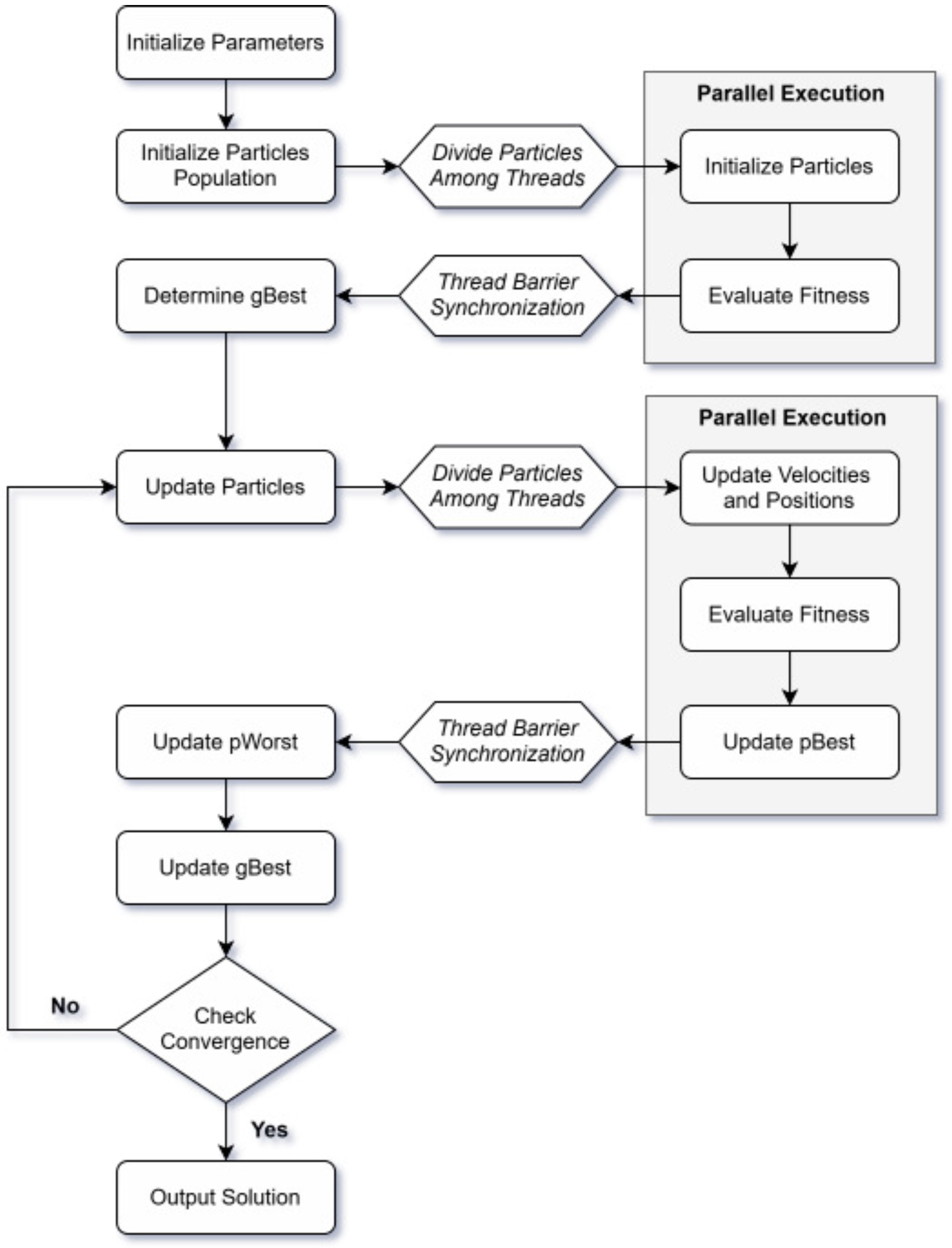
3.2. Multithreaded Design

Multithreaded algorithm design is a technique aimed at accelerating computation by dividing the workload into smaller tasks that can be processed concurrently, thereby improving execution time. This approach leverages the parallel processing capabilities of multi-core architectures to achieve significant performance gains, particularly for large-scale and computationally intensive problems.

Key factors that contribute to effective parallelism include the following: concurrency, which enables multiple tasks to be executed simultaneously across different processing units; load balancing, which ensures tasks are evenly distributed across processing units, preventing bottlenecks and optimizing performance; coordination, which manages synchronization and interaction between processing units, preventing conflicts or race conditions and ensuring proper data sharing and updates throughout the system; and data locality, which involves placing data close to the processing units that require it to minimize latency and memory access time.

The objective of the proposed multithreaded algorithm is to utilize multi-core Central Processing Units (CPUs) to reduce execution time without compromising the accuracy and convergence characteristics of the PPSO algorithm, maintaining its core structure and operational principles. This ensures that the parallelized algorithm maintains the same stopping criteria and convergence behavior as the sequential version. The pseudocode for the proposed multithreaded PPSO is presented in Algorithm 3.

Considering the proposed implementation, not all segments of the PPSO algorithm are set to run concurrently. While some parts of the algorithm are well suited for parallel processing, others require sequential execution due to inherent dependencies. Moreover, although multithreading can accelerate computation, it also introduces overheads related to thread management, synchronization, and communication. These overheads can sometimes reduce the expected performance gains, making it more efficient to execute certain tasks sequentially, especially for smaller workloads. To illustrate this, Figure 1 presents a flowchart outlining the execution pipeline of the multithreaded CPU implementation of the PPSO algorithm.

During the initial phase of PPSO, the task with the highest computational cost is particle initialization. Consequently, this task was designed to run in parallel, and its multithreaded pseudocode is shown in Algorithm 4.

In this task, each thread is responsible for initializing a candidate solution and subsequently evaluating its fitness value. Since the initialization and fitness evaluation of individual candidate solutions do not depend on other particles, they can be performed in parallel without interdependencies. This particle independence allows each thread to operate autonomously on a separate solution, enabling efficient parallelization. Although the particle initialization task is executed only once per algorithm run, the performance gains from parallel execution remain significant. This is particularly important in large-scale problems, where particle initialization can substantially impact the overall runtime and contribute to a more efficient algorithm.

Following particle initialization, the $gBest$ is determined as an isolated task. The identification of the global best particle has low computational complexity, as it essentially involves looping through the fitness array. Consequently, the overhead associated with managing threads for this simple task would negate any potential performance gains from parallel execution.

Algorithm 3 Pseudocode for multithreaded PPSO

1: /* Initialization */  2: Initialize $numVars$, $popSize$, and $maxIters$;  3: Parallel_Initialize_particles$(X,V)$;  ▹ Multithreaded particles initialization  4: Determine $gBest$;  5: $i\leftarrow 1$;  6: /* Main loop */  7: while $i\le maxIters$ do  8:   parallel for $p\leftarrow 1,popSize$ do          ▹ Multithreaded computation  9:     for $v\leftarrow 1,numVars$ do            ▹ Parallel particle update 10:       Update velocity $V_{p,v}^i$ using Equation (3); 11:       Apply velocity constraints $V_{p,v}^i$; 12:       Update position $X_{p,v}^i$ using Equation (5); 13:       Apply boundary constraints $X_{p,v}^i$; 14:     end for 15:     Evaluate fitness value $f(X_{p,v}^i)$;   ▹ Parallel objective function evaluation 16:     if $f(X_{p,v}^i)<f(pBes{t}_{p,v}^i)$ then         ▹ Parallel $pBest$ update 17:       $pBes{t}_{p,v}^i\leftarrow X_{p,v}^i$; 18:     end if 19:   end parallel for 20:   for $p\leftarrow 1,popSize$ do 21:     if $f(pBes{t}_{p,v}^i)<f(gBes{t}_v^i)$ then           ▹ Update $gBest$ 22:       $gBes{t}_v^i\leftarrow pBes{t}_{p,v}^i$; 23:     end if 24:     if $f(pBes{t}_{p,v}^i)>f(pWors{t}^i)$ then         ▹ Determine $pWorst$ 25:       $pWors{t}^i\leftarrow pBes{t}_{p,v}^i$; 26:     end if 27:   end for 28:   $l\leftarrow rand(1,numVars)$;        ▹ Select a random component of $pWorst$ 29:   Determine $pWors{t}_l^{new}$ using Equation (6); 30:   Apply boundary constraints $pWors{t}_l^{new}$; 31:   if $f(pWors{t}^{new})<f(pWors{t}^i)$ then           ▹ Update $pWorst$ 32:     $pWors{t}^i\leftarrow pWors{t}^{new}$; 33:     if $f(pWors{t}^i)<f(gBes{t}_v^i)$ then            ▹ Update $gBest$ 34:       $gBes{t}_v^i\leftarrow pWors{t}^i$; 35:     end if 36:   end if 37:   $i\leftarrow i+1$; 38: end while 39: Output the best solution found and terminate.

Algorithm 4 Multithreaded particles initialization

1: function Parallel_Initialize_particles(X, V)  2:   parallel for $p\leftarrow 1,popSize$ do          ▹ Multithreaded computation  3:     for $v\leftarrow 1,numVars$ do          ▹ Parallel particles initialization  4:       $X_{p,v}\leftarrow L{B}_v+rand()\times (U{B}_v-L{B}_v)$;  5:       $V_{p,v}\leftarrow 0$;  6:       $pBes{t}_{p,v}\leftarrow X_{p,v}$;  7:     end for  8:     Evaluate fitness value $f(X_p)$;     ▹ Parallel objective function evaluation  9:   end parallel for 10: end function

Nevertheless, the parallel execution of tasks within the PPSO main loop provides the most significant performance benefits, as improvements are compounded across iterations. In this section of the algorithm, the most computationally intensive tasks are multithreaded, namely particle updates and fitness evaluations. Since these tasks are well suited for parallel processing, the multithreaded PPSO launches a thread for each candidate solution, with each thread individually handling the update of a single particle (including velocity and position updates), followed by the evaluation of its fitness value, along with the corresponding $pBest$ update (Algorithm 3, lines 8 to 19). Although the $pBest$ update has a low computational cost, similar to the $gBest$ determination, there are no performance penalties associated with the parallel execution of this lightweight task. This is because the $pBest$ update is executed within an already active thread, thereby avoiding the overhead costs associated with additional thread management.

Following line 19 of Algorithm 3, the remaining tasks do not benefit from multithreaded execution due to their sequential nature or low computational complexity. In this section, performance improvements are achieved through computational efficiency enhancements designed to mitigate bottlenecks. For instance, in the loop at line 20, both the $gBest$ update and the determination of $pWorst$ are handled within the same iteration. This adjustment moves the $gBest$ update earlier rather than placing it at the end of the main loop. Since $pWors{t}^{new}$ can potentially become a candidate for $gBest$, an additional $gBest$ update is included at line 33 but only if $pWors{t}^{new}$ is found to be better than the previous $pWorst$. This approach enhances execution flow by eliminating redundancies and reducing unnecessary iterations, thereby contributing to improved performance.

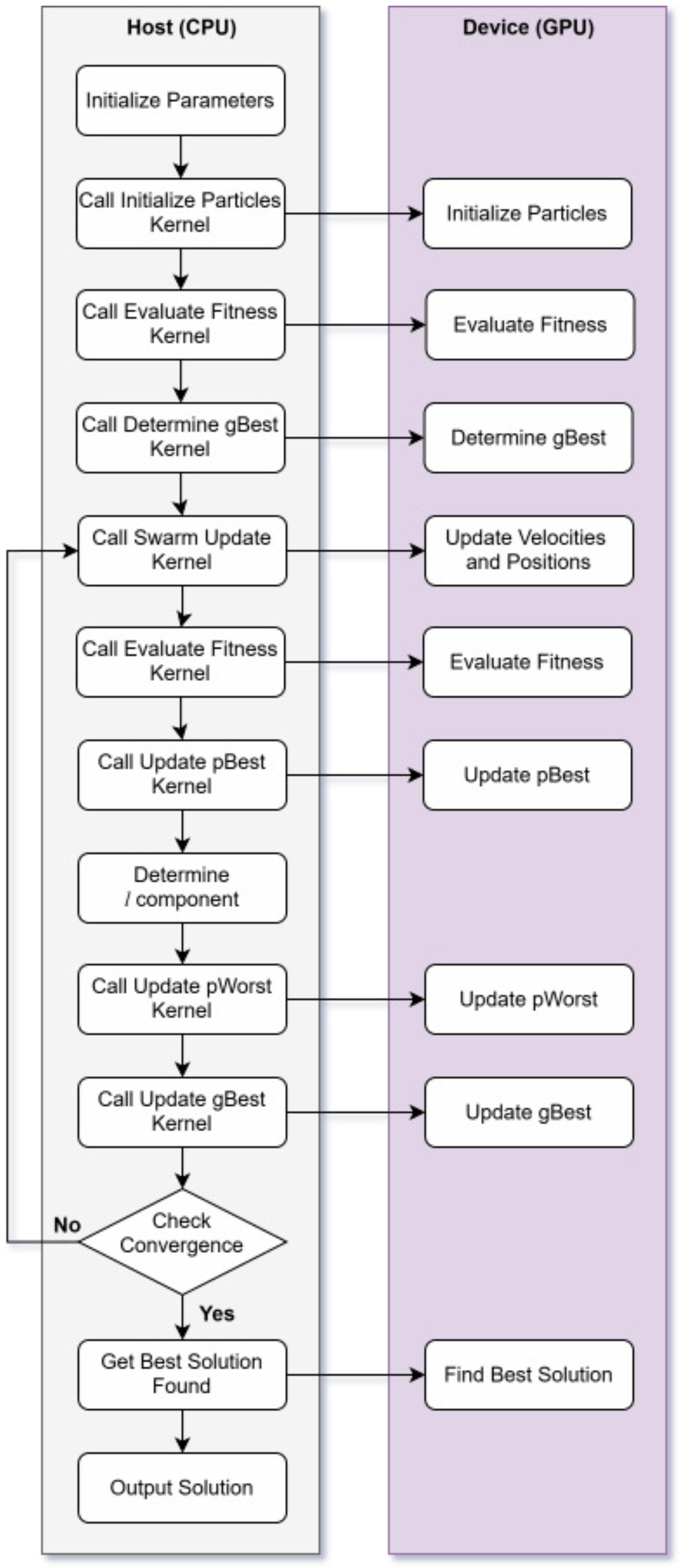
3.3. GPU Parallelization

In recent years, GPUs have emerged as powerful accelerators for high-performance computing tasks, particularly for algorithms that exhibit a high degree of parallelism.

While CPUs follow a sequential or parallel computing model with a limited number of cores, each capable of running multiple threads simultaneously, GPUs consist of thousands of smaller, simpler cores that can execute many threads in parallel, performing the same operation on multiple data points concurrently. CPUs typically rely on thread-level parallelism, prioritizing moderate parallelism, complex control flow, and high per-thread performance. In contrast, GPUs are optimized for data-level parallelism, harnessing massive parallelism to process data-parallel tasks. This makes them more effective for workloads involving simple operations on large data sets. As a result, the parallel architecture of GPUs allows them to outperform CPUs in tasks that can fully exploit this parallelism.

3.3.1. CUDA Programming Fundamentals

To enable general-purpose computing on GPUs, NVIDIA developed the Compute Unified Device Architecture (CUDA) framework, which allows programmers to offload computationally intensive tasks to the GPU. CUDA provides several key abstractions for managing parallelism, enabling both the CPU (host) and GPU (device) to collaborate effectively in a heterogeneous computing environment. The host manages overall execution, controls the flow of data, and performs sequential tasks, while the device handles the parallel computations.

Kernel functions are specialized routines designed to execute parallel tasks on the GPU. These functions decompose workloads into smaller, independent tasks that can be processed concurrently. In other words, the same code operates on different pieces of data and is executed by many threads simultaneously.

The foundational structures for organizing parallel execution on the GPU in CUDA are threads, blocks, and grids. Threads are the smallest units of execution, which are each responsible for processing a single data element. These threads are grouped into blocks, which are collections of threads that execute the same kernel instructions and can communicate and synchronize via shared memory. Multiple blocks are further organized into a grid, enabling the GPU to scale parallel execution across a large number of threads. The grid can be structured in one, two, or three dimensions, depending on the specific problem being solved. Together, these structures maximize hardware utilization and facilitate efficient data processing.

Another important aspect of GPU computation is its memory hierarchy, which plays a crucial role in determining the performance of parallel algorithms. In CUDA, memory is organized into several levels each with different characteristics in terms of size, latency, and access patterns. The main types of memory include global memory, which is large but has high latency; shared memory, which is much faster but limited in size and shared among threads within the same block; and local memory, which is private to individual threads. The efficient utilization of this hierarchy, by minimizing costly accesses to global memory and maximizing the use of shared memory, is essential for optimizing performance in GPU applications.

CUDA requires explicit memory management, as memory must be allocated and transferred between the host and device due to the heterogeneous nature of its architecture. However, data transfers between the host and device can become a bottleneck because of the relatively slow speed of the bus. To achieve optimal performance, it is necessary to minimize these transfers and keep as much data as possible on the device during execution. This strategy aligns with the principle of data locality, where data are placed closer to the processor that needs it. Additionally, designing kernels and organizing data to facilitate contiguous memory access is essential for performance. This approach enables memory coalescing, where the GPU combines multiple memory accesses into a single transaction, reducing latency and improving bandwidth efficiency, which ultimately translates into additional performance gains.

3.3.2. GPU-Based PPSO

The parallelization strategy adopted for the new GPU-based PPSO was designed to preserve the method of deriving solutions and maintain the core operating logic of the original PPSO algorithm. This ensures that any performance improvements, compared to the sequential or multithreaded implementations, are attributable solely to the applied parallelization technique rather than changes in the algorithmic approach while also preserving the same convergence characteristics and solution quality. The fundamental structure of the GPU-based PPSO is presented in Algorithm 5.

Algorithm 5 Pseudocode for GPU-based PPSO

1: /* Initialization */  2: Initialize $numVars$, $popSize$ and $maxIters$;  3: Initialize_particles_kernel$(X,V)$;  4: Evaluate_fitness_values_kernel$(X)$;  5: Determine $gBest$;  6: $i\leftarrow 1$;                             ▹ Host  7: /* Main loop */  8: while $i\le maxIters$ do                       ▹ Host  9:   Swarm_update_kernel$(X^i,V^i)$; 10:   Evaluate_fitness_values_kernel$(X^i)$; 11:   Update_pBest_kernel$(pBes{t}^i,X^i)$; 12:   $pWors{t}^i\leftarrow worst(pBes{t}^i)$; 13:   $l\leftarrow rand(1,numVars)$;                      ▹ Host 14:   $f_1\_pWors{t}^i\leftarrow f(pWors{t}^i+e_l\times {10}^{-8})$; 15:   $f_2\_pWors{t}^i\leftarrow f(pWors{t}^i-e_l\times {10}^{-8})$; 16:   Determine_pWorst_new_kernel($pWors{t}^i,l,f_1\_pWors{t}^i,f_2\_pWors{t}^i$); 17:   $f\_pWors{t}^{new}\leftarrow f(pWors{t}^{new})$ 18:   Update_pWorst_kernel($pWors{t}^{new},f\_pWors{t}^{new}$); 19:   Determine $gBes{t}^i$; 20:   $i\leftarrow i+1$;                          ▹ Host 21: end while 22: Output the best solution found and terminate.      ▹ Host and device

The GPU-based PPSO follows the heterogeneous CUDA model, where the host manages higher-level tasks, such as overseeing the computational flow, managing the structure, and launching and controlling CUDA kernels. Instances where the host is explicitly involved in the algorithm are identified with the comment host. These include controlling the main iteration loop (including initialization, termination criteria, and incrementing the loop counter, as indicated in lines 6, 8 and 20), selecting the random component of $pWorst$ (line 13), and reporting the best solution found (line 22). This is because the main iteration loop is inherently serial, serves as the computational control of the algorithm, and cannot be parallelized, making it suitable for execution on the host. Additionally, while the best solution is determined on the device, it is reported by the host, which serves as the intermediary between the device and the rest of the system. In contrast, the selection of the random component of $pWorst$ was set to be deliberately handled by the host, as the overhead of launching a kernel for such a small task would exceed the time required for the host to generate a single random number, thus negating any potential performance benefits. Figure 2 provides an overview of the execution pipeline for the GPU-based PPSO algorithm.

Similar to the CPU-based multithreaded design of PPSO, particle initialization in the GPU-based algorithm was also parallelized. However, in this case, the impact extends beyond improving the performance of the initialization phase. As discussed in Section 3.3.1, data locality plays a crucial role in performance optimization. By generating all data related to the PPSO algorithm directly on the device, the data remain close to the computational units, thereby avoiding costly transfers between host memory and the device during computation. Algorithm 6 demonstrates the operation of the particle initialization kernel.

Algorithm 6 Kernel for particle initialization

1: function Initialize_particles_kernel(X, V)  2:   /* Device code */  3:   Determine p using x dimension of $blockDim$, $blockIdx$, and $threadIdx$;  4:   if $p\le popSize$ then  5:     for $v\leftarrow 1,numVars$ do  6:       $X_{p,v}\leftarrow L{B}_v+rand()\times (U{B}_v-L{B}_v)$;  7:       $V_{p,v}\leftarrow 0$;  8:       $pBes{t}_{p,v}\leftarrow X_{p,v}$;  9:     end for 10:   end if 11: end function

This kernel operates with a one-dimensional grid of blocks where each block contains multiple threads arranged in rows. The total number of threads required for the kernel is equal to or greater than the population size. Each thread is responsible for initializing an individual particle, meaning each thread processes a separate candidate solution. This design helps prevent non-deterministic behavior, such as race conditions, which occur when multiple threads attempt to modify the same memory location simultaneously. Without proper management, such conditions can lead to unpredictable results. An additional benefit is that by assigning each thread to update a different candidate solution, the threads access contiguous memory elements, which optimizes memory coalescing and enhances memory access efficiency.

The implementation of the step Evaluate_fitness_values_kernel (lines 4 and 10 of Algorithm 5) depends on the specific SNE being addressed. In the proposed GPU parallelization, this kernel uses a structure and grid arrangement similar to that employed in the particle initialization kernel (Algorithm 6). Since determining the fitness value requires iterating over the decision variables to calculate the fitness cumulatively, this kernel uses a local variable to accumulate the sums, which minimizes accesses to global memory and improves performance.

The kernel implementation for updating the swarm (as shown in Algorithm 7) follows a design aimed at maximizing performance by utilizing CUDA’s capability to parallelize computations across thousands of threads. This is achieved through a two-dimensional grid arrangement, which enables a more efficient distribution of threads, thereby maximizing the parallel processing capabilities of the device.

The use of two dimensions (particles and decision variables) for thread indexing ensures an efficient mapping between the problem structure and the hardware, facilitating better scalability as the problem size increases (i.e., more particles and variables can be handled by larger grids). By distributing the work evenly across all available threads, each thread is assigned a clearly defined task, updating a single variable of a particle. This design requires the kernel to allocate a number of threads equal to the product of the number of particles and the number of variables. Therefore, this approach minimizes idle time for threads in the device and enables the entire swarm to be updated concurrently, considerably speeding up execution time. Since each thread operates independently on its respective particle–variable pair, race conditions and shared memory conflicts are avoided. Additionally, this design supports memory coalescing and eliminates the need for costly synchronization barriers, which would otherwise negatively impact performance.

The kernel described in Algorithm 8 is responsible for updating the $pBest$ values of the particles. Each $pBest$ update is handled independently by a separate thread using 1D thread indexing, requiring at least as many threads as the size of the particle population.

Algorithm 7 Kernel for swarm updating

1: function Swarm_update_kernel(X, V)  2:   /* Device code */  3:   Determine p using x dimension of $blockDim$, $blockIdx$, and $threadIdx$;  4:   Determine v using y dimension of $blockDim$, $blockIdx$, and $threadIdx$;  5:   if $p\le popSize$ and $v\le numVar$ then  6:     $V_{p,v}^{new}\leftarrow (2\times rand()-0.5)\times V_{p,v}+(2\times rand()-0.5)\times$         $(pBes{t}_{p,v}-X_{p,v})+(2\times rand()-0.5)\times (gBes{t}_v-X_{p,v})$; ▹ Equation (3)  7:     Velocity_constraint$(V_{p,v}^{new});$  8:     $\omega \leftarrow (2\times rand()-0.5)\times (gBes{t}_v-pBes{t}_{p,v})+(2\times rand()-0.5)\times$       $(gBes{t}_v-X_{p,v})$;                  ▹ Equation (4)  9:     $X_{p,v}^{new}\leftarrow pBes{t}_{p,v}+(2\times rand()-0.5)\times V_{p,v}^{new}+(2\times rand()-0.5)\times \omega$; ▹ Equation (5) 10:     Boundary_constraint$(X_{p,v}^{new});$ 11:     /* Update particle */ 12:     $X_{p,v}\leftarrow X_{p,v}^{new}$; 13:     $V_{p,v}\leftarrow V_{p,v}^{new}$; 14:   end if 15: end function

Algorithm 8 Kernel for updating $pBest$

1: function Update_pBest_kernel($pBest$, X)  2:   /* Device code */  3:   Determine p using x dimension of $blockDim$, $blockIdx$, and $threadIdx$;  4:   if $p\le popSize$ then  5:     if $f(X_p)<f(pBes{t}_p)$ then  6:       for $v\leftarrow 1,numVars$ do  7:         $pBes{t}_{p,v}\leftarrow X_{p,v}$;  8:       end for  9:     end if 10:   end if 11: end function

This kernel requires the precomputation of the fitness values, meaning that the kernel only needs to compare these precomputed fitness values, which is a much simpler operation. This approach eliminates potential sources of branch divergence, which occur when threads follow different execution paths based on the fitness evaluation, leading to inefficient execution. As a result, the kernel focuses solely on comparing fitness values and updating the $pBest$ values, ensuring that all threads follow the same execution path and thus improving overall efficiency.

To determine $pWorst$ (line 12 of Algorithm 5), the particle with the highest value of $f(pBes{t}_p)$ must be identified. Since the fitness values have already been evaluated in a previous step (line 10 of Algorithm 5), this process becomes computationally lightweight. It only involves identifying the index corresponding to the maximum value in the fitness array, as there is a one-to-one correspondence between fitness values and particles. The identified index then references the $pWorst$ particle within the swarm.

The computational procedures for the determination of $pWors{t}^{new}$ and updating the $pWorst$ in the swarm (lines 16 and 18 of Algorithm 5) exhibit inherent sequential characteristics, as these operations involve modifying a single array index, specifically the previously determined random component (index l) of $pWorst$. Due to these structural constraints, the core functions involved are inherently unsuitable for parallel execution. As a result, the kernels Determine_pWorst_new_kernel Algorithm 9) and Update_pWorst_kernel Algorithm 10) are configured for sequential execution, using a grid dimension of 1 block and 1 thread. Despite their inherently serial nature, performing these computations on the GPU provides performance benefits. Specifically, this process benefits from improved data locality because the necessary data remain resident on the device. This setup minimizes the need for costly device-to-host and host-to-device memory transfers, which would otherwise introduce latency and degrade performance.

Algorithm 9 Kernel for determining $pWors{t}^{new}$

1: function Determine_pWorst_new_kernel($pWorst$, l, $f_1\_pWorst$, $f_2\_pWorst$) 2:   /* Device code */ 3:   $pWors{t}_l^{new}\leftarrow pWors{t}_l+(2\times rand()-0.5)\times {\displaystyle \frac{f_1\_pWorst-f_2\_pWorst}{2\times {10}^{-8}\times (U{B}_l-L{B}_l)}}$  ▹ Equation (6) 4:   Boundary_constraint$(pWors{t}_l^{new});$ 5: end function

Algorithm 10 Kernel for updating $pWorst$

1: function Update_pWorst_kernel($pWors{t}^{new}$, $f\_pWors{t}^{new}$) 2:   /* Device code */ 3:   if $f\_pWors{t}^{new}<f(pWorst)$ then 4:     $pWors{t}_l\leftarrow pWors{t}_l^{new}$; 5:   end if 6: end function

It is important to note that both of these kernels rely on prior evaluations of the components $f_1\_pWors{t}^i$, $f_2\_pWors{t}^i$, and $f_{p}Wors{t}^{new}$, which are performed in parallel. Additionally, in Algorithm 10, although the fitness of the initial (unmodified) $pWorst$ is represented as a function for clarity and ease of understanding, its value already resides in device memory, having been computed during the parallel fitness evaluation of the entire swarm (line 10 of Algorithm 5), making recalculation unnecessary.

4. Computational Experiments

This section outlines the experimental setup, including the hardware and software configurations used for benchmarking the algorithms and the test parameters. It also presents the scalable SNE test problems employed to evaluate performance.

4.1. Experimental Setup

The proposed implementations were developed using the Julia programming language [28], version 1.11.0 (released on 7 October 2024), which was selected for its high-performance capabilities and user-friendly syntax, particularly in scientific computing. Its Just-In-Time (JIT) compilation ensures execution speeds comparable to those of low-level languages [29], while its syntax is especially well suited for mathematical and optimization tasks. As an open-source alternative to proprietary tools like MATLAB, Julia offers flexibility and accessibility for research and development. GPU acceleration was achieved using CUDA.jl [30] version 5.5.2, using CUDA runtime version 12.6. Julia’s built-in support for both multithreading and GPU computing enables efficient parallel execution on modern hardware architectures, making it a suitable platform for implementing both multithreaded CPU and GPU-accelerated algorithms.

The computational setup used for testing includes an AMD EPYC 7643 CPU, featuring 48 cores and 96 threads, along with 32 GB of DDR4 RAM and an NVIDIA A100 PCIe GPU, featuring 6912 CUDA cores and 80 GB of HBM2e VRAM. This server-grade hardware configuration enables a comprehensive evaluation of both the multithreaded CPU and GPU-based implementations of the algorithm. Therefore, the benchmarking results accurately reflect the performance of modern hardware platforms and facilitate a thorough analysis of scalability and efficiency across the different parallelization strategies.

The performance of the algorithms was evaluated using test parameters that reflect a range of problem sizes. The problem dimensions varied from 1000 to 5000 in increments of 1000, and the population size was set to 10 times the problem dimension, ensuring a sufficiently large search space for the optimization process. The stopping criterion for all experiments was set at 1000 iterations, providing a fixed benchmark for performance comparisons. To evaluate the reliability and robustness of the algorithms, 31 independent runs were performed for each test configuration, ensuring that the results account for variability and are statistically significant.

Since Julia relies on a JIT compilation process, this often results in longer execution times during the program’s first run. To ensure the integrity of the computational analysis, an additional warm-up run was introduced to absorb the delay caused by the JIT compiler, allowing subsequent runs to provide more reliable performance metrics.

The computations for both the CPU multithreaded and GPU-based implementations were conducted using double-precision floating-point arithmetic to ensure high accuracy in the results. However, in the GPU testing, additional tests with single-precision floating-point arithmetic were also conducted to explore the trade-offs between computational speed and precision.

All the computational times reported in this work encompass the entire execution of the algorithm, including all phases from initialization to the final reporting of the best solution found. This comprehensive measurement is critical for assessing performance in both CPU multithreading and GPU-based implementations, as it captures the full range of computational costs associated with the algorithm. This methodology ensures that the true performance improvements or trade-offs are fully captured, allowing for a fair and meaningful comparison between the sequential and parallelized approaches.

In this study, the boundary constraint technique applied to the update of particle positions in PPSO was value clamping, which utilizes the upper and lower bounds of the search space to ensure that candidate solutions remain within the defined domain. This technique effectively prevents particles from exploring regions outside the search space. Additionally, a similar constraint was applied to the particle velocities with the maximum velocity for each design variable set to 10% of the range of the search space.

4.2. Test Problems

Ten scalable SNEs were used to evaluate the performance of the proposed algorithms. These test problems were selected from the existing literature due to their complexity and their ability to scale with problem dimensions, ensuring a robust assessment of the algorithms across different levels of complexity. The mathematical expressions for the benchmark functions are presented below, along with the corresponding domain and specific values for the variables involved in these functions, providing a detailed description of the problem setup.

Problem 1.

(Broyden tridiagonal function [31], $n=1000,2000,3000,4000,5000$)

$f_1(\mathit{x})=(3-2x_1)x_1-2x_2+1$,

$f_n(\mathit{x})=(3-2x_n)x_n-x_{n-1}+1$,

$f_i(\mathit{x})=(3-2x_i)x_i-x_{i-1}-2x_{i+1}+1,i=2,\dots ,n-1$,

$D={([-1,1],\dots ,[-1,1])}^T$.

Problem 2.

(Discrete boundary value function [31], $n=1000,2000,3000,4000,5000$)

$f_1(\mathit{x})=2x_1-x_2+h^2{(x_1+h+1)}^3/2$,

$f_n(\mathit{x})=2x_n-x_{n-1}+h^2{(x_n+nh+1)}^3/2$,

$f_i(\mathit{x})=2x_i-x_{i-1}-x_{i+1}+h^2{(x_i+t_i+1)}^3/2,$ $i=2,\dots ,n-1,$

where $h={\displaystyle \frac{1}{n+1}}$ and $t_i=ih$,

$D={([0,5],\dots ,[0,5])}^T$.

Problem 3.

(Extended Powell singular function [31], $n=1000,2000,3000,4000,5000$)

$f_{4i-3}(\mathit{x})=x_{4i-3}+10x_{4i-2}$,

$f_{4i-2}(\mathit{x})=\sqrt{5}(x_{4i-1}-x_{4i})$,

$f_{4i-1}(\mathit{x})={(x_{4i-2}-2x_{4i-1})}^2$,

$f_{4i}(\mathit{x})=\sqrt{10}{(x_{4i-3}-x_{4i})}^2,i=1,\dots ,5$,

$D={([-100,100],\dots ,[-100,100])}^T$.

Problem 4.

(Modified Rosenbrock function [32], $n=1000,2000,3000,4000,5000$)

${\displaystyle f_{2i-1}(\mathit{x})=\frac{1}{1+exp(-x_{2i-1})}-0.73}$,

$f_{2i}(\mathit{x})=10(x_{2i}-x_{2i-1}^2),i=1,\dots ,{\displaystyle \frac{n}{2}}$,

$D={([-10,10],\dots ,[-10,10])}^T$.

Problem 5.

(Powell badly scaled function [32], $n=1000,2000,3000,4000,5000$)

$f_{2i-1}(\mathit{x})={10}^4{x}_{2i-1}{x}_{2i}-1$,

$f_{2i}(\mathit{x})=exp(-x_{2i-1})+exp(-x_{2i})-1.0001,i=1,\dots ,{\displaystyle \frac{n}{2}}$,

$D={([0,100],\dots ,[0,100])}^T$.

Problem 6.

(Schubert–Broyden function [33], $n=1000,2000,3000,4000,5000$)

$f_1(\mathit{x})=(3-x_1)x_1+1-2x_2$,

$f_n(\mathit{x})=(3-x_n)x_n+1-x_{n-1}$,

$f_i(\mathit{x})=(3-x_i)x_i+1-x_{i-1}-2x_{i+1},i=2,\dots ,n-1$,

$D={([-100,100],\dots ,[-100,100])}^T$.

Problem 7.

(Martínez function [34], $n=1000,2000,3000,4000,5000$)

$f_1(\mathit{x})=(3-0.1x_1)x_1+1-2x_2+x_1$,

$f_n(\mathit{x})=(3-0.1x_n)x_n+1-2x_{n-1}+x_n$,

$f_i(\mathit{x})=(3-0.1x_i)x_i+1-x_{i-1}-2x_{i+1}+x_1,i=2,\dots ,n-1$,

$D={([-100,100],\dots ,[-100,100])}^T$.

Problem 8.

(Extended Rosenbrock function [31], $n=1000,2000,3000,4000,5000$)

$f_{2i-1}(\mathit{x})=10(x_{2i}-x_{2i-1}^2)$,

$f_{2i}(\mathit{x})=1-x_{2i-1},i=1,\dots ,{\displaystyle \frac{n}{2}}$,

$D={([-100,100],\dots ,[-100,100])}^T$.

Problem 9.

(Bratu’s problem [35], $n=1000,2000,3000,4000,5000$)

$f_1(\mathit{x})=-2x_1+x_2+\alpha h^{2}exp(x_1)$,

$f_n(\mathit{x})=x_{n-1}-2x_n+\alpha h^{2}exp(x_n)$,

${\displaystyle f_i(\mathit{x})=x_{i-1}-2x_i+x_{i+1}+\alpha h^{2}exp(x_i)}$, $i=2,\dots ,n-1$,

where $h={\displaystyle \frac{1}{n+1}}$ and $\alpha \ge 0$ is a parameter; here $\alpha =3.5$,

$D={([-100,100],\dots ,[-100,100])}^T$.

Problem 10.

(The beam problem [35], $n=1000,2000,3000,4000,5000$)

$f_1(\mathit{x})=-2x_1+x_2+\alpha h^{2}sin(x_1)$,

$f_n(\mathit{x})=x_{n-1}-2x_n+\alpha h^{2}sin(x_n)$,

${\displaystyle f_i(\mathit{x})=x_{i-1}-2x_i+x_{i+1}+\alpha h^{2}exp(x_i)}$, $i=2,\dots ,n-1$,

where $h={\displaystyle \frac{1}{n+1}}$ and $\alpha \ge 0$ is a parameter; here $\alpha =11$,

$D={([-100,100],\dots ,[-100,100])}^T$.

5. Results and Discussion

In this section, a detailed analysis of the performance and behavior of the proposed PPSO implementations is presented. The results are evaluated against both sequential and multithreaded CPU implementations, focusing on assessing computational efficiency and scalability across various problem dimensions. To provide a comprehensive understanding of the performance improvements achieved through parallelization, the discussion is divided into four key areas: an evaluation of the optimization of sequential algorithm codebases (Section 5.1); a comparison between the sequential and multithreaded CPU implementations (Section 5.2); an analysis of the performance benefits from GPU parallelization (Section 5.3); and an evaluation of the impact of parallelization on the quality of solutions obtained (Section 5.4).

Each of these subsections delves into specific aspects of the performance metrics, including computation time, speedup factors, and the overall effectiveness of different hardware architectures. The speedup (S) metric used to quantify performance improvement is defined as the ratio of the time taken to complete a task in a reference scenario, typically that of sequential computation ($T_{\mathrm{sequential}}$), to the time taken to complete the same task via parallel execution ($T_{\mathrm{parallel}}$). Mathematically, this relationship is expressed as

$$S={\displaystyle \frac{T_{\mathrm{sequential}}}{T_{\mathrm{parallel}}}}.$$

(7)

5.1. Sequential Codebase Evaluation

The three sequential algorithm codebases, referred to as codebases A, B, and C, were described earlier in Section 3.1. Their performance evaluation results are presented in

Table 1. Performance testing of the sequential algorithm codebases (computation time in seconds; estimated total memory allocation in gibibytes, GiB).

Dim.	Codebase A		Codebase B		Codebase C
	Time	Mem. Alloc.	Time	Mem. Alloc.	Time	Mem. Alloc.
1000	39.40	91.31	25.97	23.17	15.53	23.17
2000	190.71	362.25	131.21	91.93	60.42	91.93
3000	591.18	812.32	388.96	206.29	165.73	206.29
4000	1046.19	1442.42	646.16	366.24	282.66	366.24
5000	1860.78	2252.52	1123.96	571.80	451.98	571.80

. The test parameters include a warm-up run, followed by the mean of three test runs, with algorithm execution limited to 100 iterations, a population size set to 10 times the problem dimension, and the use of the same random seed in all tests.

Empirical testing shows that code optimization in codebase B reduced the mean memory footprint of codebase A by approximately 74.6%, which was a reduction also achieved by codebase C. Although the column-major order optimization in codebase C improves cache locality, it did not result in any further enhancement of memory allocation efficiency. Overall, these improvements led to substantial reductions in computational time: codebase B achieved an approximate 35.5% mean computational time reduction compared to codebase A, while codebase C nearly doubled the performance improvement, achieving an approximate 69.9% reduction in mean computational time compared to codebase A. These findings underscore the importance of memory-efficient techniques in both memory management and algorithmic optimizations, highlighting their critical role in achieving substantial performance improvements, particularly in large-scale computational problems.

Based on these results, codebase C was selected for sequential testing and served as a well-optimized foundation for the multithreaded implementation due to its superior performance in comparison to the other codebases.

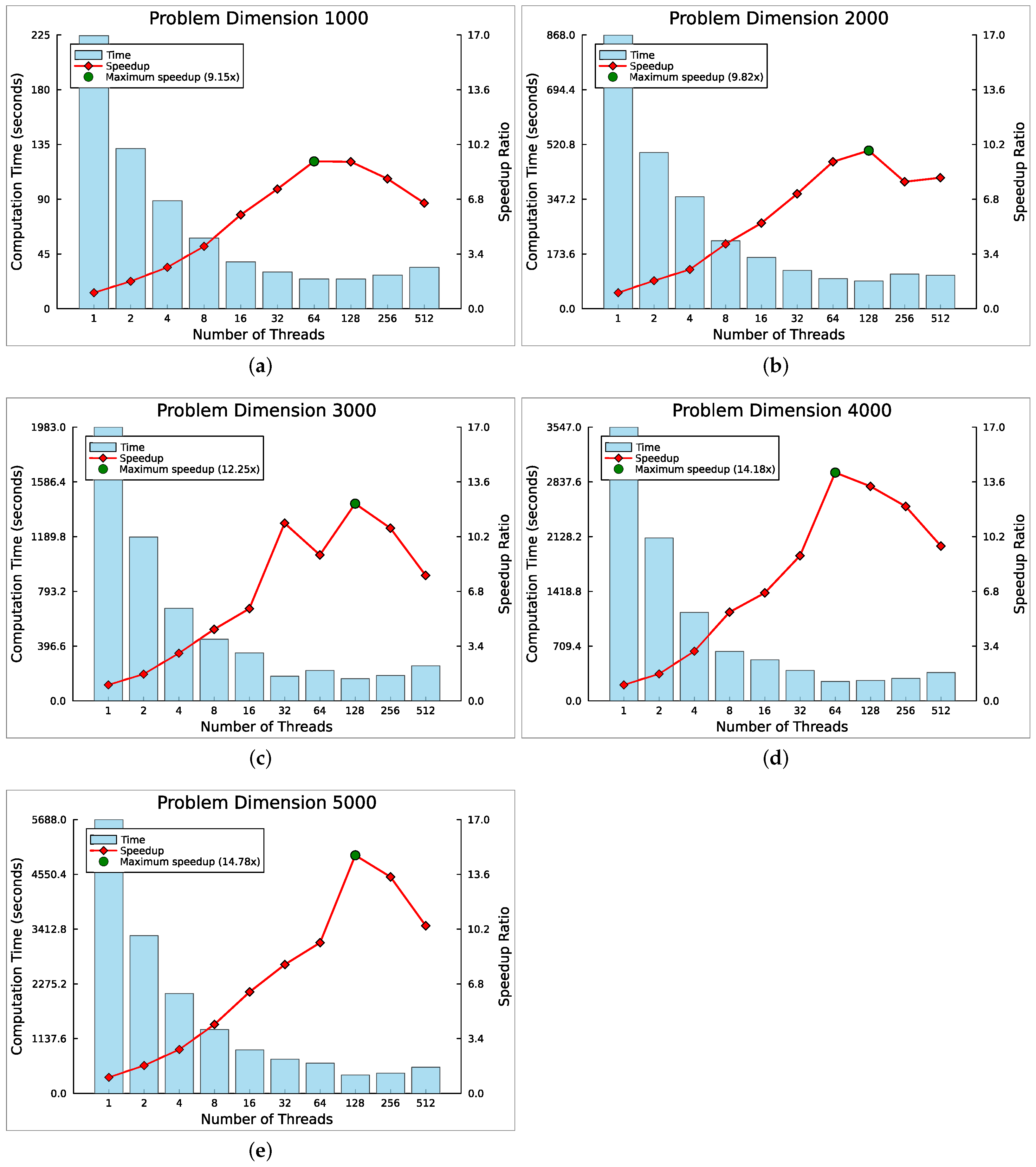
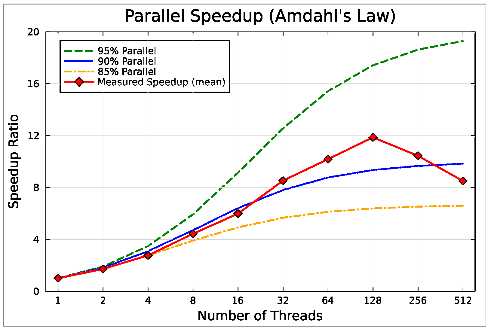
5.2. Multithreaded Speedup Analysis

Table 2. PPSO CPU performance metrics from sequential execution up to 16 threads (computation time in seconds; speedup values normalized to sequential execution).

Dim. (Pop.)	Prob. No.	Sequential	2 Threads		4 Threads		8 Threads		16 Threads
		Time	Time	Speedup	Time	Speedup	Time	Speedup	Time	Speedup
1000 (10,000)	1	201.41	120.91	1.67	90.15	2.23	51.74	3.89	33.66	5.98
	2	216.32	115.79	1.87	76.07	2.84	45.38	4.77	38.49	5.62
	3	234.27	140.83	1.66	89.69	2.61	56.81	4.12	40.35	5.81
	4	249.61	150.81	1.66	129.61	1.93	64.23	3.89	38.86	6.42
	5	261.86	159.72	1.64	92.97	2.82	64.18	4.08	40.66	6.44
	6	260.06	147.47	1.76	99.19	2.62	62.88	4.14	41.28	6.30
	7	212.39	117.39	1.81	76.26	2.79	60.18	3.53	41.37	5.13
	8	198.72	116.87	1.70	64.44	3.08	56.80	3.50	35.67	5.57
	9	201.59	120.13	1.68	80.06	2.52	57.38	3.51	41.26	4.89
	10	208.11	127.47	1.63	89.40	2.33	61.94	3.36	33.94	6.13
2000 (20,000)	1	767.34	460.99	1.66	320.42	2.39	202.56	3.79	147.12	5.22
	2	790.30	457.53	1.73	373.53	2.12	230.84	3.42	144.54	5.47
	3	922.04	511.71	1.80	386.10	2.39	241.97	3.81	159.45	5.78
	4	984.43	543.32	1.81	374.24	2.63	226.54	4.35	175.02	5.62
	5	1029.65	558.05	1.85	417.97	2.46	209.94	4.90	179.61	5.73
	6	1032.13	535.42	1.93	381.07	2.71	247.36	4.17	178.52	5.78
	7	776.92	477.41	1.63	361.04	2.15	189.00	4.11	159.37	4.87
	8	784.83	460.56	1.70	297.90	2.63	199.57	3.93	155.47	5.05
	9	801.32	504.44	1.59	330.48	2.42	218.60	3.67	157.27	5.10
	10	785.91	445.81	1.76	312.49	2.52	192.38	4.09	172.37	4.56
3000 (30,000)	1	1748.95	1111.85	1.57	620.75	2.82	361.14	4.84	371.09	4.71
	2	1814.80	1170.25	1.55	702.31	2.58	428.42	4.24	322.14	5.63
	3	2135.45	1253.57	1.70	766.84	2.78	491.18	4.35	305.04	7.00
	4	2296.83	1323.15	1.74	706.72	3.25	509.21	4.51	323.22	7.11
	5	2400.22	1328.41	1.81	629.89	3.81	470.68	5.10	399.22	6.01
	6	2286.73	1354.65	1.69	706.57	3.24	441.18	5.18	341.90	6.69
	7	1762.67	1068.86	1.65	655.59	2.69	392.28	4.49	352.98	4.99
	8	1786.70	1139.72	1.57	553.59	3.23	460.88	3.88	347.58	5.14
	9	1825.84	1091.53	1.67	723.73	2.52	484.34	3.77	348.35	5.24
	10	1771.69	1029.75	1.72	648.64	2.73	434.49	4.08	371.13	4.77
4000 (40,000)	1	3155.91	2138.04	1.48	1050.57	3.00	625.43	5.05	428.97	7.36
	2	3271.58	2026.97	1.61	1100.51	2.97	631.93	5.18	511.64	6.39
	3	3730.62	2444.81	1.53	1206.68	3.09	646.50	5.77	618.50	6.03
	4	4046.10	2322.71	1.74	1239.92	3.26	683.88	5.92	593.46	6.82
	5	4081.88	2317.78	1.76	1248.15	3.27	715.32	5.71	483.43	8.44
	6	4246.33	2329.60	1.82	1399.72	3.03	648.33	6.55	546.88	7.76
	7	3349.56	1831.52	1.83	996.56	3.36	620.19	5.40	562.44	5.96
	8	3184.82	1856.79	1.72	1151.81	2.77	628.52	5.07	448.32	7.10
	9	3234.49	1932.52	1.67	1025.79	3.15	606.86	5.33	544.59	5.94
	10	3164.82	1918.81	1.65	1050.31	3.01	616.30	5.14	603.06	5.25
5000 (50,000)	1	5021.38	2844.10	1.77	1904.56	2.64	1325.81	3.79	949.56	5.29
	2	5299.68	3060.97	1.73	2006.01	2.64	1312.41	4.04	823.62	6.43
	3	5863.39	3258.24	1.80	2197.87	2.67	1331.35	4.40	877.68	6.68
	4	6378.36	3632.83	1.76	2276.32	2.80	1307.49	4.88	970.52	6.57
	5	7109.06	3727.13	1.91	2206.63	3.22	1434.24	4.96	854.76	8.32
	6	6593.87	3920.42	1.68	2195.36	3.00	1278.81	5.16	906.08	7.28
	7	5055.14	3143.65	1.61	2070.81	2.44	1331.02	3.80	967.73	5.22
	8	4975.48	3074.87	1.62	1941.05	2.56	1316.31	3.78	915.10	5.44
	9	5334.54	3236.17	1.65	2023.51	2.64	1312.60	4.06	926.00	5.76
	10	5242.86	2899.70	1.81	1940.35	2.70	1325.12	3.96	869.98	6.03

and

Table 3. PPSO CPU performance metrics across 32 to 512 threads (computation time in seconds; speedup values normalized to sequential execution).

Dim. (Pop.)	Prob. No.	32 Threads		64 Threads		128 Threads		256 Threads		512 Threads
		Time	Speedup	Time	Speedup	Time	Speedup	Time	Speedup	Time	Speedup
1000 (10,000)	1	27.92	7.21	22.78	8.84	23.91	8.42	26.94	7.48	33.40	6.03
	2	28.03	7.72	22.93	9.44	23.97	9.02	27.40	7.89	33.59	6.44
	3	30.25	7.74	27.78	8.43	24.53	9.55	27.92	8.39	34.95	6.70
	4	28.44	8.78	24.34	10.25	25.25	9.89	28.95	8.62	35.45	7.04
	5	29.43	8.90	25.94	10.09	25.68	10.20	29.35	8.92	35.78	7.32
	6	36.90	7.05	24.75	10.51	25.88	10.05	29.05	8.95	35.16	7.40
	7	31.79	6.68	26.96	7.88	24.01	8.85	27.02	7.86	33.03	6.43
	8	31.05	6.40	23.08	8.61	24.18	8.22	27.18	7.31	33.14	6.00
	9	28.53	7.07	22.56	8.94	23.97	8.41	26.80	7.52	33.75	5.97
	10	30.69	6.78	24.44	8.52	24.02	8.66	26.85	7.75	33.05	6.30
2000 (20,000)	1	129.92	5.91	93.91	8.17	87.30	8.79	115.24	6.66	103.14	7.44
	2	118.60	6.66	102.17	7.74	86.04	9.19	113.60	6.96	101.68	7.77
	3	125.61	7.34	82.16	11.22	88.47	10.42	112.39	8.20	107.80	8.55
	4	120.85	8.15	109.58	8.98	89.55	10.99	107.42	9.16	111.42	8.84
	5	120.09	8.57	93.49	11.01	91.00	11.32	108.69	9.47	111.83	9.21
	6	136.40	7.57	97.54	10.58	89.24	11.57	107.76	9.58	111.47	9.26
	7	117.39	6.62	94.47	8.22	86.84	8.95	104.51	7.43	104.26	7.45
	8	104.04	7.54	87.01	9.02	87.24	9.00	109.28	7.18	101.79	7.71
	9	131.42	6.10	90.95	8.81	86.58	9.26	109.85	7.29	103.70	7.73
	10	114.04	6.89	104.57	7.52	90.16	8.72	113.84	6.90	106.12	7.41
3000 (30,000)	1	167.15	10.46	220.41	7.93	157.03	11.14	182.99	9.56	258.71	6.76
	2	183.91	9.87	243.53	7.45	147.74	12.28	183.46	9.89	226.33	8.02
	3	169.17	12.62	240.12	8.89	164.02	13.02	186.65	11.44	253.86	8.41
	4	190.38	12.06	224.11	10.25	169.21	13.57	189.96	12.09	264.32	8.69
	5	183.40	13.09	208.84	11.49	168.15	14.27	188.92	12.70	257.03	9.34
	6	192.63	11.87	230.44	9.92	166.35	13.75	186.48	12.26	258.85	8.83
	7	173.75	10.14	220.78	7.98	157.87	11.17	181.32	9.72	250.56	7.03
	8	178.76	10.00	226.44	7.89	161.30	11.08	182.41	9.79	250.76	7.13
	9	187.34	9.75	159.95	11.41	161.41	11.31	181.39	10.07	265.72	6.87
	10	168.93	10.49	238.39	7.43	162.53	10.90	181.93	9.74	259.03	6.84
4000 (40,000)	1	381.39	8.27	242.53	13.01	260.82	12.10	290.97	10.85	366.04	8.62
	2	378.23	8.65	238.70	13.71	261.82	12.50	289.19	11.31	358.13	9.14
	3	357.62	10.43	254.85	14.64	264.31	14.11	293.43	12.71	364.70	10.23
	4	409.03	9.89	244.19	16.57	275.37	14.69	302.41	13.38	381.04	10.62
	5	350.41	11.65	383.72	10.64	275.99	14.79	298.89	13.66	371.79	10.98
	6	462.64	9.18	250.30	16.96	274.12	15.49	300.29	14.14	367.62	11.55
	7	374.81	8.94	232.30	14.42	261.46	12.81	291.79	11.48	358.15	9.35
	8	414.10	7.69	223.61	14.24	261.54	12.18	289.36	11.01	373.34	8.53
	9	384.84	8.40	243.35	13.29	260.32	12.43	290.12	11.15	381.78	8.47
	10	449.09	7.05	221.43	14.29	261.20	12.12	286.27	11.06	364.99	8.67
5000 (50,000)	1	688.06	7.30	620.70	8.09	378.51	13.27	416.26	12.06	543.04	9.25
	2	679.29	7.80	689.92	7.68	382.58	13.85	418.82	12.65	525.77	10.08
	3	687.51	8.53	706.20	8.30	390.09	15.03	423.05	13.86	554.37	10.58
	4	745.23	8.56	459.96	13.87	408.44	15.62	431.74	14.77	573.91	11.11
	5	802.39	8.86	711.26	10.00	401.30	17.71	435.18	16.34	561.62	12.66
	6	731.70	9.01	671.43	9.82	359.64	18.33	429.11	15.37	533.68	12.36
	7	594.42	8.50	672.33	7.52	383.46	13.18	415.23	12.17	545.24	9.27
	8	712.45	6.98	687.94	7.23	376.80	13.20	417.81	11.91	555.96	8.95
	9	664.33	8.03	402.47	13.25	384.21	13.88	421.06	12.67	522.12	10.22
	10	811.77	6.46	671.32	7.81	380.80	13.77	415.60	12.62	546.21	9.60

provide detailed performance overviews of the proposed PPSO implementations on the CPU, from sequential execution to multithreaded execution using 2 to 512 threads, across various test scenarios. These tables present the mean computation times from 31 independent runs for each test scenario alongside the corresponding improvement ratios relative to the sequential execution.

The results demonstrate that employing multiple threads to run the algorithm leads to a significant reduction in total computation time. The rate of improvement, however, varies based on both the number of threads used and the specific test parameters. Specifically, the speedup factors observed ranged from a modest improvement of 1.48$\times$ with 2 threads, for test problem number 1 with a dimension of 4000, to a more substantial 18.33$\times$ with 128 threads for test problem number 6 with a dimension of 5000.

When analyzing the mean computational times, a general decrease is observed with the use of additional processing threads with a more pronounced reduction occurring during the initial multithreaded tests. This is consistent with the expected benefits of parallelization, where distributing the computation across multiple threads allows for more efficient execution and reduced processing time. This trend is clearly illustrated in Figure 3, where the mean computational times are presented for each problem dimension along with the corresponding mean speedup achieved in each multithreading configuration.

For SNEs with a dimension of 1000, the results shown in Figure 3a reveal that the mean computational times reach a plateau with 64 threads. At this configuration, the maximum mean speedup of 9.15$\times$ is achieved for this problem dimension, suggesting that the multithreaded implementation is highly parallelizable, effectively using the additional threads to maximize the utilization of available processing resources. However, beyond 128 threads, diminishing returns in speedup are observed, indicating that the algorithm is no longer able to efficiently utilize the additional processing resources. Based on this test setup, the use of 64 threads is recommended, as it offers the optimal processing performance.

Upon increasing the problem dimension to 2000 (Figure 3b), the performance analysis reveals a generally similar trend, although the peak mean speedup shifts to 128 threads with a slightly higher ratio of 9.82$\times$ achieved. This result indicates that increasing the computational workload by doubling the problem dimension (and the population size) allows the algorithm to continue benefiting from additional threads, resulting in further performance gains up to a higher thread count threshold. This shift in the optimal thread count suggests that larger problem dimensions require greater parallel processing capacity to achieve maximum efficiency.

Beyond 128 threads, the speedup gains taper off, indicating that further increases in thread count fail to produce significant performance improvements even with increased workloads.

Figure 3c, illustrating problem dimension 3000, demonstrates a notable surge in the mean speedup ratio when increasing the thread count from 16 to 32, resulting in a performance improvement of approximately 92.6%. This improvement can be attributed to factors such as enhanced load balancing, which ensures a more even distribution of the workload and reduces idle times, as well as improved cache efficiency and better utilization of the CPU’s memory hierarchy. However, when the thread count is increased further, from 32 to 64, a decrease of 21.7% in the mean speedup is observed, indicating diminishing returns for this particular workload and thread combination. This reduction in performance may be attributed to overhead from thread synchronization or memory access contention. Nonetheless, a subsequent improvement of 35.1% in speedup is attained when moving to 128 threads, resulting in the optimal configuration for this workload with a maximum mean speedup of 12.25$\times$. This suggests that while the algorithm may continue to benefit from additional threads in certain scenarios, it is ultimately constrained by the system’s hardware and architecture.

The mean speedup of 14.18$\times$ was achieved when processing SNEs with 4000 variables using 64 threads, as shown in Figure 3d. Notably, despite the increased computational workload compared to the previous problem dimension of 3000, the peak speedup was achieved at a lower thread count. This suggests that for this specific problem dimension, the algorithm makes more efficient use of processing resources up to 64 threads, beyond which additional threads result in diminishing returns, limiting further scaling of the computation. Additionally, there was a substantial increase of approximately 57.3% in speedup when moving from 32 threads to 64 threads, indicating that a larger parallelizable portion of the problem remained that could be better exploited. When averaging the multithreaded results per problem dimension (see the last column of

Table 4. Multithreaded mean speedup for each problem dimension. The final row shows the mean speedup across all assessed dimensions, and the last column displays the mean speedup across all multithreaded tests.

Dim.	2 T	4 T	8 T	16 T	32 T	64 T	128 T	256 T	512 T	Mean
1000	1.71	2.58	3.88	5.83	7.43	9.15	9.13	8.07	6.56	6.04
2000	1.75	2.44	4.02	5.32	7.13	9.13	9.82	7.88	8.14	6.18
3000	1.67	2.97	4.44	5.73	11.03	9.07	12.25	10.73	7.79	7.30
4000	1.68	3.09	5.51	6.71	9.02	14.18	13.32	12.07	9.62	8.35
5000	1.73	2.73	4.28	6.30	8.00	9.36	14.79	13.44	10.41	7.89
Mean	1.71	2.76	4.43	5.98	8.52	10.18	11.86	10.44	8.50

), the 4000-dimensional problem demonstrates the highest mean speedup overall. This indicates that for the computational experiments conducted, the proposed multithreaded implementation achieves a balance between computational workload and processing efficiency at this dimensionality.

The highest mean speedup of 14.79$\times$ across all test scenarios was achieved when processing SNEs with 5000 variables using 128 threads, as shown in Figure 3e. At this dimensionality, the computational peak shifts back to 128 threads compared to 64 threads in the previous problem size. Additionally, the most significant increase in speedup with increasing thread count now occurs when transitioning from 64 to 128 threads, rather than the previous jump from 32 to 64 threads, although with a comparable improvement of approximately 58%. This observation suggests that the increased computational workload benefits from a greater number of threads, enabling more effective parallelization through a more balanced distribution of the workload across the available threads.

An analysis of the mean results by problem dimension revealed no consistent pattern in the number of threads required to achieve maximum speedup with the optimal number alternating between 64 and 128 threads. This variation can be attributed to the scaling characteristics of the algorithm for different problem sizes as well as the strengths and limitations of the system’s hardware. While smaller problem sizes generally benefit from fewer threads and larger problems require additional threads to fully exploit parallelism, other factors, such as the nature of the problem and its potential for parallelization, influence thread scalability efficiency as well.

A more detailed compilation of the aggregate mean speedup ratios is provided in Table 4, which aids in determining the optimal thread configuration for these particular experiments and test setup. Considering the overall means across all assessed dimensions, the data indicate that the multithreaded implementation of PPSO achieves its highest mean speedup of 11.86$\times$ at 128 threads, suggesting this configuration represents the optimal balance between parallel workload and system overhead for the presented use case. Overall, the results demonstrate an increasing efficiency of the parallelized algorithm from 2 to 128 threads with the mean speedup consistently rising as more threads are utilized. However, further increases in thread count fail to yield additional improvements, as evidenced by diminishing returns observed at 256 and 512 threads. This suggests that factors such as memory or I/O constraints may begin to limit performance as the number of threads increases.

Figure 4 further contextualizes the mean aggregated speedups by comparing them to the theoretical speedup predictions based on Amdahl’s law [36] for varying degrees of parallelism (85%, 90%, and 95%). Amdahl’s law models the potential speedup of a parallelized application based on the proportion of code that can be parallelized and the number of threads utilized. It assumes that a portion of the code is inherently serial and cannot benefit from parallelization, thereby limiting the overall achievable speedup.

When comparing the mean measured speedup across different thread counts to the theoretical predictions, the results show that the multithreaded implementation of PPSO closely follows the speedup curve for 90% parallelizable code up to 16 threads. From 32 to 256 threads, the measured speedup exceeds the 90% parallelization prediction, indicating that in the lower range of thread counts, the implementation is more notably affected by the serial portion of the algorithm. This outcome aligns with the implementation strategy of the multithreaded PPSO (Algorithm 3), where the most computationally intensive parts of the algorithm were designed to run in parallel, incorporating the structural and memory management enhancements introduced by the codebase optimization.

As the number of threads increases, the parallel portion of the work becomes more prominent, resulting in a higher parallelization factor. This result indicates that the algorithm is highly parallelizable and continues to benefit from increased thread counts. The highest observed speedup occurs at 128 threads, indicating that this is the optimal thread count for the given implementation and workload. At this point, the balance between the parallel workload and overhead is optimal, maximizing efficiency while minimizing bottlenecks such as memory contention or synchronization delays.

Although at 256 threads the speedup results still exceed the 90% parallelization prediction, the improvements begin to regress, becoming closer to the results obtained at 64 threads. As the number of threads increases further to 512, the speedup declines further, falling below the theoretical speedup predicted by Amdahl’s Law for 90%-parallelizable code. This performance drop reflects the diminishing returns typically associated with high thread counts, where the overhead of managing a large number of threads becomes significant. Contributing factors likely include increased thread synchronization overhead, cache contention, memory bandwidth saturation, and inefficiencies in thread management. These factors can negate the benefits of adding more threads, resulting in suboptimal scaling at higher thread counts.

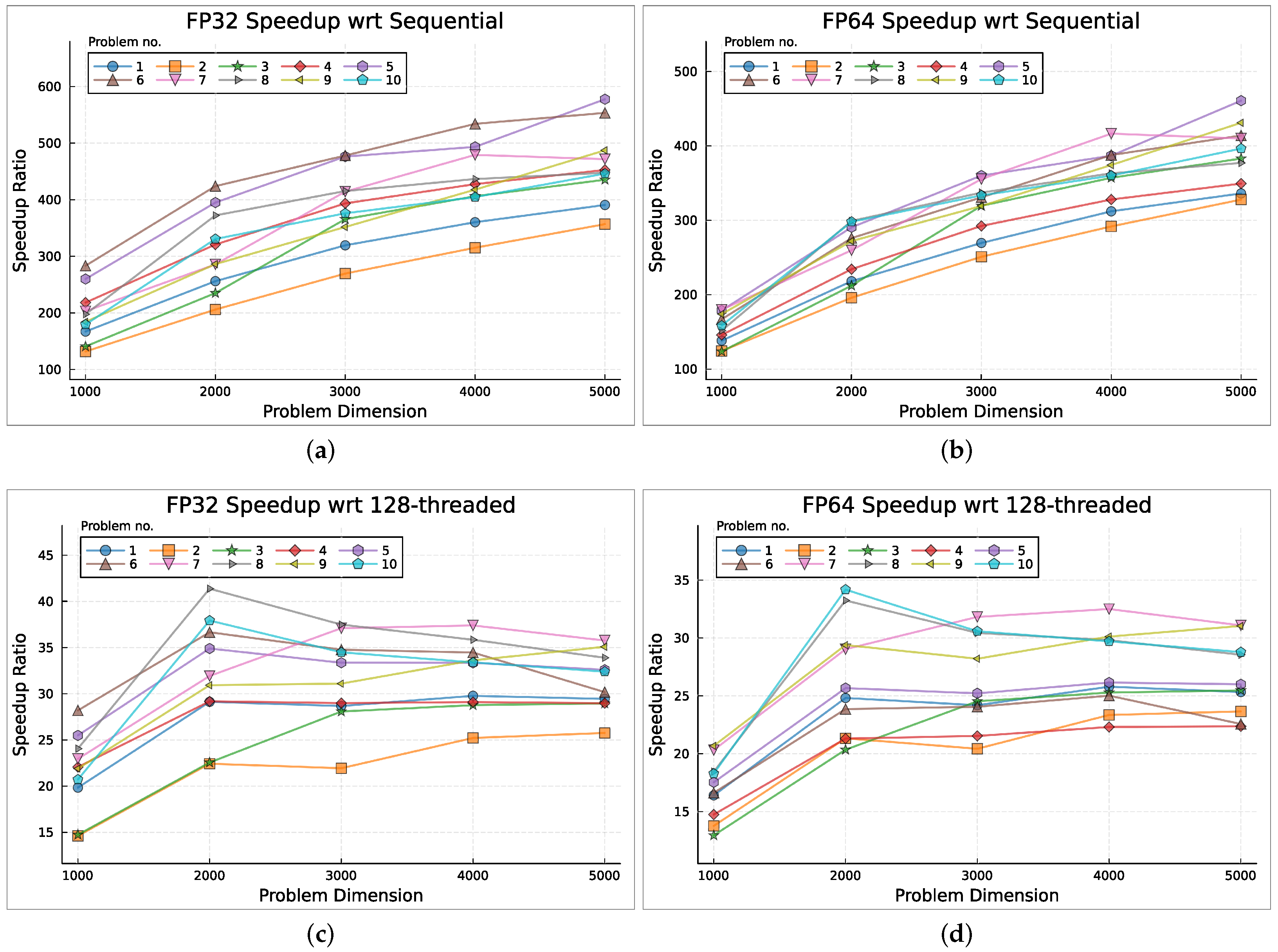
5.3. GPU Parallelization

An overview of the mean performance metrics for the proposed GPU parallelization of PPSO, derived from individual runs and tested using both single-precision (FP32) and double-precision (FP64) arithmetic, are provided in

Table 5. GPU-parallelized PPSO performance metrics using single and double-precision arithmetic. Computation time is reported in seconds, and speedup values are normalized with respect to both sequential and 128-threaded (i.e., best-performing multithreaded) executions.

Dim. (Pop.)	Prob. No.	Single Precision (FP32)			Double Precision (FP64)
		Time	Speedup (Seq.)	Speedup (128 T)	Time	Speedup (Seq.)	Speedup (128 T)
1000 (10,000)	1	1.21	167.12	19.84	1.46	138.20	16.41
	2	1.64	131.88	14.62	1.74	124.25	13.77
	3	1.66	140.76	14.74	1.89	123.69	12.95
	4	1.14	218.23	22.07	1.71	145.82	14.75
	5	1.01	259.87	25.49	1.47	178.71	17.53
	6	0.92	283.33	28.20	1.56	166.96	16.62
	7	1.05	203.06	22.95	1.18	179.77	20.32
	8	1.00	197.74	24.06	1.31	151.62	18.45
	9	1.09	184.21	21.90	1.16	173.94	20.68
	10	1.16	179.53	20.72	1.31	158.45	18.29
2000 (20,000)	1	3.00	256.08	29.13	3.52	218.13	24.82
	2	3.84	206.01	22.43	4.03	195.91	21.33
	3	3.92	235.11	22.56	4.35	212.13	20.35
	4	3.07	320.82	29.18	4.20	234.23	21.31
	5	2.61	394.92	34.90	3.54	290.52	25.67
	6	2.43	423.95	36.66	3.74	275.97	23.86
	7	2.72	285.67	31.93	2.99	259.66	29.03
	8	2.11	372.25	41.38	2.62	299.05	33.24
	9	2.80	286.23	30.93	2.95	271.99	29.39
	10	2.38	330.61	37.93	2.64	298.00	34.18
3000 (30,000)	1	5.48	319.39	28.68	6.49	269.47	24.19
	2	6.73	269.50	21.94	7.23	250.92	20.43
	3	5.84	365.62	28.08	6.69	319.35	24.53
	4	5.84	393.45	28.99	7.86	292.37	21.54
	5	5.04	476.24	33.36	6.67	360.03	25.22
	6	4.78	477.99	34.77	6.91	330.76	24.06
	7	4.26	414.23	37.10	4.96	355.27	31.82
	8	4.30	415.28	37.49	5.30	337.17	30.44
	9	5.19	351.76	31.10	5.72	319.12	28.21
	10	4.71	375.97	34.49	5.31	333.39	30.58
4000 (40,000)	1	8.76	360.28	29.78	10.11	312.02	25.79
	2	10.38	315.14	25.22	11.21	291.72	23.35
	3	9.19	406.13	28.77	10.45	357.02	25.29
	4	9.46	427.51	29.10	12.34	327.86	22.31
	5	8.27	493.30	33.35	10.56	386.72	26.15
	6	7.95	533.98	34.47	10.95	387.63	25.02
	7	6.99	479.16	37.40	8.04	416.37	32.50
	8	7.30	436.51	35.85	8.77	362.99	29.81
	9	7.74	417.75	33.62	8.64	374.19	30.12
	10	7.82	404.63	33.40	8.79	360.02	29.71
5000 (50,000)	1	12.85	390.67	29.45	14.94	336.03	25.33
	2	14.85	356.81	25.76	16.17	327.77	23.66
	3	13.47	435.29	28.96	15.31	382.90	25.47
	4	14.09	452.57	28.98	18.26	349.28	22.37
	5	12.31	577.46	32.60	15.43	460.66	26.00
	6	11.92	553.32	30.18	15.93	413.86	22.57
	7	10.72	471.57	35.77	12.33	409.87	31.09
	8	11.12	447.59	33.90	13.20	377.03	28.55
	9	10.95	487.26	35.09	12.38	430.97	31.04
	10	11.75	446.12	32.40	13.23	396.30	28.78

. In the context of GPU speedup assessment, the inclusion of both floating-point precision formats is particularly relevant, as the performance characteristics of GPU computation can vary substantially between FP32 and FP64. This approach facilitates a more comprehensive evaluation of GPU efficiency across different workloads while assessing the trade-off between computational speed and numerical accuracy. Additionally, the improvement ratios were calculated relative to both the sequential execution and the best-performing multithreaded execution, providing a more thorough assessment of the performance gains achieved through GPU parallelization.

The observations demonstrate consistent performance, indicating that the GPU parallelization of the PPSO algorithm leads to significant computational time reductions compared to both sequential and multithreaded CPU implementations. Furthermore, the speedup tends to be greater for larger dimensions, suggesting that the parallelization strategy efficiently distributes the workload across the available resources.

The speedup normalized against the sequential CPU execution, as expected, produces the greatest performance improvements. Specifically, in this comparison, the speedup values for the GPU-based PPSO implementation range from 131.88$\times$ to 577.46$\times$ with a mean of 356.60$\times$ using FP32 arithmetic and from 123.69$\times$ to 460.66$\times$ with a mean of 294.52$\times$ when employing FP64 arithmetic.

When comparing the GPU parallelization of PPSO with the best-performing multithreaded algorithm execution (which, according to previous results, was achieved with 128 threads), the observed improvement ratios are more modest yet still significant. When normalized to the 128-thread multithreaded CPU execution, the speedups achieved by the GPU-based PPSO range from 14.62$\times$ to 41.38$\times$ with a mean of 29.63$\times$ for FP32 operations and from 12.95$\times$ to 34.18$\times$ with a mean of 24.58$\times$ for FP64 operations.

The findings demonstrate that FP32 consistently outperforms FP64 across all measurements. Specifically, based on the mean speedup results, FP32 offers an empirical performance advantage of approximately 21% compared to FP64 in both sequential and 128-threaded speedup normalizations. Considering the A100 GPU’s 2:1 FP32-to-FP64 performance ratio, this 21% gap may seem relatively modest. However, in optimization algorithms, performance bottlenecks often arise from memory access, synchronization overhead, or inter-core communication rather than arithmetic unit saturation. Furthermore, architectural aspects of the A100 GPU, which is optimized for high FP64 throughput (unlike consumer-grade GPUs), help mitigate the performance advantage of FP32.

It is important to emphasize that the choice between FP32 and FP64 is heavily dependent on the specific use case. While FP32 offers a performance benefit, this may not always justify the potential risks associated with reduced computational precision. In applications where fitness function evaluations are sensitive to numerical accuracy, or where the optimization problem involves narrow or highly constrained optimal regions, the precision loss from using FP32 could substantially impact the solution quality. In such cases, the accurate representation of problem parameters and results using FP64 may override the computational speed benefits of FP32.

Figure 5 illustrates the problem-specific behavior of the GPU-based PPSO, showcasing the performance of the algorithm for varying problem dimensions. This representation aids in understanding how the computational load of each problem affects speedup and how this speedup evolves across different problem sizes.

Examining the progression of speedup relative to sequential CPU performance for both FP32 and FP64 arithmetic (Figure 5a,b), the results reveal a positive scaling trend with increasing problem size for most test problems. However, problem number 7 exhibited a slight speedup regression at the 5000-dimensional problem when computed with both floating-point precisions. This regression suggests diminishing returns, likely due to a reduction in the computational effort required for this problem, which causes the parallel computation to become less efficient and insufficient to offset the costs associated with launching and managing a larger number of threads.

The problems that perform best on average for FP32 precision are problems 6 and 5 with mean speedups of 454.52$\times$ and 440.36$\times$, respectively. For FP64, problem 5 stands out with the highest mean result of 335.33$\times$, which is followed by problem 7 at 324.19$\times$. Regarding the least efficient problems, problem 2 is the worst performer, followed by problem 1, for both computational precisions. The mean speedups for these problems are 255.87$\times$ and 298.71$\times$ for FP32 and 238.11$\times$ and 254.77$\times$ for FP64, respectively.

The analysis of these results highlights consistent performance trends, particularly among the least efficient problems, while revealing notable variability among the best-performing ones. Notably, problem 5, which ranks among the top performers in both arithmetic precisions, shifts from being the best performer in FP64 to the second-best performer in FP32. Furthermore, the general performance profiles for the test problems by problem dimensions remain largely consistent across FP32 and FP64, though there are shifts in performance rankings. These shifts suggest that the computational effort for certain problems is more influenced by arithmetic overheads than by problem size or dimensionality alone.

The speedup results relative to 128-threaded CPU for FP32 and FP64 arithmetic, as depicted in Figure 5c,d, exhibit fluctuating trends as the workload increases, indicating variations in scaling behavior. Similar to the speedup results observed relative to sequential CPU performance, the performance behavior of the test problems remains largely consistent across varying problem dimensions for both arithmetic precisions, though some reordering of performance rankings is observed.

As computational complexity increases to the 2000-dimensional problem, positive scaling is observed across all test problems for both FP32 and FP64 computations. At this point, problems 8 and 10 achieve their maximum speedup, which is followed by negative scaling beyond this threshold. Conversely, problems 4 and 7 achieve their maximum speedup at a higher complexity, specifically at the 4000-dimensional problem. After the negative scaling between problem dimensions 2000 and 3000, problems 2 and 9 show an upward trend in the remaining problem dimensions, suggesting potential for further scaling beyond the 5000-dimensional problem. The remaining test problems either reach a saturation point at the 2000-dimensional mark—where performance improvements plateau and no further measurable gains are achieved—or exhibit a more fluctuating trend with speedup oscillating between increasing and decreasing phases as computational complexity grows. Despite the positive speedup ratios, these fluctuations suggest diminishing returns as problem complexity continues to scale.

The general speedup trend with increasing workload for both computational precisions is presented in Figure 6 where the mean GPU-based parallelization performance is compared against single-threaded and 128-threaded CPU computations.

In the left plot of Figure 6, the positive scaling of speedup with increasing problem dimension is observed. This indicates that as the problem size grows, the parallel efficiency of the GPU implementation improves substantially, particularly in comparison to sequential CPU execution. This suggests that the GPU-based algorithm benefits from larger workloads, where its high degree of parallelism can be utilized more effectively, leading to more efficient computation and higher speedups. Additionally, it is clear that the gap between FP32 and FP64 computations widens as the problem size increases. This implies that single-precision arithmetic better exploits GPU resources at higher computational loads, achieving greater speedups compared to double precision. This is likely because FP32 requires fewer computational resources, such as memory bandwidth, and places a lower computational demand on arithmetic units than FP64.

Regarding the mean speedup relative to 128-threaded CPU execution (right plot of Figure 6), the initial trend shows a steady increase in speedup, which is followed by a saturation point after the 2000-dimensional problem. Beyond this point, further increases in computational complexity lead to small fluctuations in speedup, which is characterized by an oscillating pattern. This suggests that the GPU-based algorithm is no longer able to scale effectively and has entered a region of diminishing returns. This behavior is likely due to the GPU reaching a performance ceiling relative to the 128-threaded CPU. After the 2000 problem size, the GPU is unable to deliver substantial performance improvements, which is possibly because it has already optimized the use of its available resources. Consequently, further increases in problem size do not yield proportional gains in GPU performance, signaling a limit to the scalability of the algorithm relative to the 128-threaded CPU. This trend is observed in both FP32 and FP64, indicating that the diminishing returns are not necessarily due to computational limitations but rather to the inherent constraints of the parallelization strategy and the available hardware resources at larger problem sizes.

5.4. Parallelization Impact on Solution Quality

In some cases, parallelization techniques may impact the quality of optimization solutions, potentially leading to suboptimal results due to issues such as synchronization errors.

Table 6. Impact of multithreaded and GPU-based parallelization on PPSO solution quality: percentage relative difference in mean best solutions compared to the sequential CPU baseline.

Dim.	CPU									GPU
	2 T	4 T	8 T	16 T	32 T	64 T	128 T	256 T	512 T	FP64
1000	1.16	−0.21	−0.21	−0.09	0.30	−3.41	2.63	4.69	−0.18	−1.03
2000	0.36	2.19	2.19	2.33	−0.61	1.17	0.10	−0.12	−0.70	1.50
3000	−0.51	−0.09	−0.09	0.57	0.73	2.13	1.24	1.12	1.46	−1.94
4000	1.98	0.58	0.58	2.30	4.09	0.82	2.17	3.34	2.32	2.50
5000	−0.11	−0.12	−0.12	−0.29	1.51	−0.97	−1.62	−0.13	2.14	−0.63
Mean	0.58	0.47	0.47	0.96	1.21	−0.05	0.90	1.78	1.01	0.08

provides a detailed analysis of the impact of both multithreaded CPU and GPU-based parallelization on the quality of the solutions obtained by the PPSO algorithm. The table shows the percentage relative difference in the mean best solutions found compared to the baseline mean best solutions obtained from the sequential CPU tests. Since the multithreaded tests only utilized double-precision arithmetic, the quality assessment of solutions found with FP32 computation using GPU-based parallelization is omitted from the comparison. Nevertheless, the expected results should be equivalent, as the computations in both FP32 and FP64 used the same algorithm implementation with the only modification being the variable types corresponding to each precision.

Table 6 shows that the percentage relative difference in the mean solution ranges from −0.09% to 4.69%, indicating a relatively small deviation from the solutions obtained with sequential optimization. When considering the mean results across all problem dimensions, the mean percentage relative difference further narrows to a range of −0.05% to 1.78%, highlighting even smaller discrepancies. Comparing the results from parallel computation using both multithreaded and GPU-based approaches, the data reveal that GPU computation did not result in a higher percentage difference in the solutions, performing among the best in terms of solution accuracy.

Variation in the obtained solutions is to be expected when working with optimization algorithms like PPSO. Given the stochastic nature of such algorithms, the best solutions may vary between runs due to factors such as random initialization, their non-deterministic behavior, and the size and complexity of the optimization problems. These factors often lead to fluctuations in convergence patterns. Considering the challenging nature of solving SNEs, along with the large problem dimensions tested (ranging from 1000 to 5000 variables), the percentage relative difference of the mean best solutions found falls well within the expected range for computational experiments of this type. This suggests that the proposed multithreaded and GPU-based parallel implementations of PPSO not only adhere to the same operating principles and yield similar results as the sequential algorithmic implementation but also effectively and substantially reduce the computation time.

6. Conclusions

The results of this study underscore the advantages of leveraging modern hardware platforms, including multicore processors and high-efficiency GPUs, to accelerate the resolution of complex optimization problems using intelligent population-based algorithms, particularly swarm-inspired methods like PSO and its variations, including the modified PSO algorithm considered here. These findings provide valuable insights into the practical implications of parallel computing for solving large-scale SNEs as nonlinear optimization problems, enabling these algorithms to address the complexity of solving such systems effectively and efficiently.

Relatively to multithreaded parallelization, the results obtained indicate that increasing the number of threads initially delivers substantial performance improvements with processing times decreasing significantly as more threads are utilized. However, beyond an optimal thread count, the performance benefits diminish due to overheads from thread management and resource contention, highlighting the trade-offs inherent in multithreaded computation.

The most notable finding in the multithreaded results is that the highest mean speedup of 11.86$\times$ was achieved with 128 threads with speedups ranging from 8.42$\times$ to 18.33$\times$. This corresponds to the point of optimal performance, suggesting that 128 threads represent the ideal count for the specific algorithm, the problems considered, and the CPU configuration used in this study. At this point, the system likely achieves a balance between the benefits of parallel execution and the overheads associated with managing higher thread counts.

As the number of threads increases further, particularly at 256 and 512 threads, the speedup starts to decrease. At 256 threads, the mean speedup drops to 10.44$\times$, and at 512 threads, it further declines to 8.50$\times$. This trend reflects diminishing returns in parallel processing, where increasing the number of threads beyond a certain point introduces overhead that negates performance gains. Several factors may contribute to this, including CPU core saturation, inefficient load balancing, and increased synchronization overhead.

Regarding the effectiveness of the GPU parallelization, the GPU-based PPSO demonstrated significant performance improvements compared to sequential execution. In this analysis, the speedup ranged from 123.69$\times$ to 460.66$\times$ with a mean of 294.52$\times$ when performing double-precision arithmetic and from 131.88$\times$ to 577.46$\times$ with a mean of 356.60$\times$ for single-precision arithmetic. This additional performance gain of nearly 21% in single-precision computing comes with the trade-off of reduced computational precision, making its use case-dependent for performance-critical applications. The observations also revealed a correlation between increased problem size (or workload) and improved speedup, demonstrating effective scalability. These results highlight the computational efficiency of the GPU-based PPSO, particularly in handling large-scale optimization problems.

To provide additional context for assessing the overall efficiency of the GPU-based implementation, the results were compared with the highest-performing multithreaded CPU execution (with 128 threads). The measured speedup ranged from 12.95$\times$ to 34.18$\times$ with a mean of 24.58$\times$ using double-precision arithmetic and from 14.62$\times$ to 41.38$\times$ with a mean of 29.63$\times$ for single-precision. In this analysis, the speedup growth exhibited fluctuations as the workload increased beyond the 2000-dimensional problem. This behavior is likely caused by the GPU reaching a performance ceiling when compared to the 128-threaded CPU, because it cannot provide significant performance gains. While the GPU-based algorithm consistently outperforms the CPU, its performance shows diminishing returns for very high-dimensional problems, which is likely because it has already utilized nearly all of its available resources.

The impact of parallelization on solution quality was also evaluated. The mean percentage difference in the solutions obtained through both parallelizations ranged from $-0.05$% to 1.78%, on average, indicating a minimal deviation in solution quality between the sequential and parallel approaches. This suggests that the algorithms perform similarly. These results confirm the correctness of the parallelizations and that the core operating principles of the original PPSO algorithm were preserved.

This research also highlights the critical importance of algorithmic efficiency and memory optimization in computational tasks. Optimizing the sequential codebase resulted in significant improvements, reducing the memory footprint by as much as 74.6% and decreasing computational time by nearly 70%. By evaluating the performance of the parallel implementations against a highly optimized sequential algorithm, the results become more transparent, highlighting the actual speedup gains achieved through parallelization.

References

1. Kennedy, J.; Eberhart, R. Particle swarm optimization. In Proceedings of the ICNN’95–International Conference on Neural Networks, Perth, WA, Australia, 27 November–1 December 1995; Volume 4, pp. 1942–1948. [Google Scholar] [CrossRef]
2. Zaini, F.A.; Sulaima, M.F.; Razak, I.A.W.A.; Zulkafli, N.I.; Mokhlis, H. A review on the applications of PSO-based algorithm in demand side management: Challenges and opportunities. IEEE Access 2023, 11, 53373–53400. [Google Scholar] [CrossRef]
3. Holland, J.H. Adaptation in Natural and Artificial Systems: An Introductory Analysis with Applications to Biology, Control, and Artificial Intelligence; MIT Press: Cambridge, MA, USA, 1992. [Google Scholar] [CrossRef]
4. Storn, R. Differential Evolution—A Simple and Efficient Adaptive Scheme for Global Optimization over Continuous Spaces; Technical Report 11; International Computer Science Institute: Berkeley, CA, USA, 1995. [Google Scholar]
5. Storn, R.; Price, K. Differential evolution—A simple and efficient heuristic for global optimization over continuous spaces. J. Glob. Optim 1997, 11, 341–359. [Google Scholar] [CrossRef]
6. Dorigo, M.; Birattari, M.; Stutzle, T. Ant colony optimization. IEEE Comput. Intell. Mag. 2006, 1, 28–39. [Google Scholar] [CrossRef]
7. Shami, T.M.; El-Saleh, A.A.; Alswaitti, M.; Al-Tashi, Q.; Summakieh, M.A.; Mirjalili, S. Particle swarm optimization: A comprehensive survey. IEEE Access 2022, 10, 10031–10061. [Google Scholar] [CrossRef]
8. Jaberipour, M.; Khorram, E.; Karimi, B. Particle swarm algorithm for solving systems of nonlinear equations. Comput. Math. Appl. 2011, 62, 566–576. [Google Scholar] [CrossRef]
9. Kotsireas, I.S.; Pardalos, P.M.; Semenov, A.; Trevena, W.T.; Vrahatis, M.N. Survey of methods for solving systems of nonlinear equations, Part I: Root-finding approaches. arXiv 2022. [Google Scholar] [CrossRef]
10. Li, Y.; Wei, Y.; Chu, Y. Research on solving systems of nonlinear equations based on improved PSO. Math. Probl. Eng. 2015, 2015, 727218. [Google Scholar] [CrossRef]
11. Choi, H.; Kim, S.D.; Shin, B.C. Choice of an initial guess for Newton’s method to solve nonlinear differential equations. Comput. Math. Appl. 2022, 117, 69–73. [Google Scholar] [CrossRef]
12. Zhang, G.; Allaire, D.; Cagan, J. Taking the guess work out of the initial guess: A solution interval method for least-squares parameter estimation in nonlinear models. J. Comput. Inf. Sci. Eng. 2020, 21, 021011. [Google Scholar] [CrossRef]
13. Dattner, I. A model-based initial guess for estimating parameters in systems of ordinary differential equations. Biometrics 2015, 71, 1176–1184. [Google Scholar] [CrossRef] [PubMed]
14. Gong, W.; Liao, Z.; Mi, X.; Wang, L.; Guo, Y. Nonlinear equations solving with intelligent optimization algorithms: A survey. Complex Syst. Model. Simul. 2021, 1, 15–32. [Google Scholar] [CrossRef]
15. Verma, P.; Parouha, R.P. Solving systems of nonlinear equations using an innovative hybrid algorithm. Iran. J. Sci. Technol. Trans. Electr. Eng. 2022, 46, 1005–1027. [Google Scholar] [CrossRef]
16. Tawhid, M.A.; Ibrahim, A.M. An efficient hybrid swarm intelligence optimization algorithm for solving nonlinear systems and clustering problems. Soft Comput. 2023, 27, 8867–8895. [Google Scholar] [CrossRef]
17. Ribeiro, S.; Silva, B.; Lopes, L.G. Solving systems of nonlinear equations using Jaya and Jaya-based algorithms: A computational comparison. In Algorithms for Intelligent Systems, Proceedings of the International Conference on Paradigms of Communication, Computing and Data Analytics (PCCDA 2023), New Delhi, India, 22–23 April 2023; Yadav, A., Nanda, S.J., Lim, M.H., Eds.; Springer: Singapore, 2023; pp. 119–136. [Google Scholar] [CrossRef]
18. Silva, B.; Lopes, L.G.; Mendonça, F. Parallel GPU-acceleration of metaphorless optimization algorithms: Application for solving large-scale nonlinear equation systems. Appl. Sci. 2024, 14, 5349. [Google Scholar] [CrossRef]
19. Tiwari, P.; Mishra, V.N.; Parouha, R.P. Modified differential evolution to solve systems of nonlinear equations. OPSEARCH 2024, 61, 1968–2001. [Google Scholar] [CrossRef]
20. Lalwani, S.; Sharma, H.; Satapathy, S.C.; Deep, K.; Bansal, J.C. A survey on parallel particle swarm optimization algorithms. Arab. J. Sci. Eng. 2019, 44, 2899–2923. [Google Scholar] [CrossRef]
21. Hussain, M.M.; Fujimoto, N. GPU-based parallel multi-objective particle swarm optimization for large swarms and high dimensional problems. Parallel Comput. 2020, 92, 102589. [Google Scholar] [CrossRef]
22. Wang, C.C.; Ho, C.Y.; Tu, C.H.; Hung, S.H. cuPSO: GPU parallelization for particle swarm optimization algorithms. In Proceedings of the 37th ACM/SIGAPP Symposium on Applied Computing, Virtual, 25–29 April 2022; ACM: New York, NY, USA, 2022; pp. 1183–1189. [Google Scholar] [CrossRef]
23. Wang, H.; Luo, X.; Wang, Y.; Sun, J. Identification of heat transfer coefficients in continuous casting by a GPU-based improved comprehensive learning particle swarm optimization algorithm. Int. J. Therm. Sci. 2023, 190, 108284. [Google Scholar] [CrossRef]
24. Chraibi, A.; Ben Alla, S.; Touhafi, A.; Ezzati, A. Run time optimization using a novel implementation of Parallel-PSO for real-world applications. In Proceedings of the 2020 5th International Conference on Cloud Computing and Artificial Intelligence: Technologies and Applications (CloudTech), Marrakesh, Morocco, 24–26 November 2020; pp. 1–7. [Google Scholar] [CrossRef]
25. Kumar, L.; Pandey, M.; Ahirwal, M.K. Implementation and testing of parallel PSO to attain speedup on general purpose computer systems. Multimed. Tools Appl. 2024, 83. [Google Scholar] [CrossRef]
26. Liao, S.; Liu, B.; Cheng, C.; Li, Z.; Wu, X. Long-term generation scheduling of hydropower system using multi-core parallelization of particle swarm optimization. Water Resour. Manag. 2017, 31, 2791–2807. [Google Scholar] [CrossRef]
27. Engelbrecht, A. Particle swarm optimization: Velocity initialization. In Proceedings of the 2012 IEEE Congress on Evolutionary Computation, Brisbane, QLD, Australia, 10–15 June 2012; pp. 1–8. [Google Scholar] [CrossRef]
28. Bezanson, J.; Edelman, A.; Karpinski, S.; Shah, V.B. Julia: A fresh approach to numerical computing. SIAM Rev. 2017, 59, 65–98. [Google Scholar] [CrossRef]
29. Gao, K.; Mei, G.; Piccialli, F.; Cuomo, S.; Tu, J.; Huo, Z. Julia language in machine learning: Algorithms, applications, and open issues. Comput. Sci. Rev. 2020, 37, 100254. [Google Scholar] [CrossRef]
30. Besard, T.; Foket, C.; De Sutter, B. Effective extensible programming: Unleashing Julia on GPUs. IEEE Trans. Parallel Distrib. Syst. 2019, 30, 827–841. [Google Scholar] [CrossRef]
31. Moré, J.J.; Garbow, B.S.; Hillstrom, K.E. Testing unconstrained optimization software. ACM Trans. Math. Softw. 1981, 7, 17–41. [Google Scholar] [CrossRef]
32. Friedlander, A.; Gomes-Ruggiero, M.A.; Kozakevich, D.N.; Martínez, J.M.; Santos, S.A. Solving nonlinear systems of equations by means of quasi-Newton methods with a nonmonotone strategy. Optim. Methods Softw. 1997, 8, 25–51. [Google Scholar] [CrossRef]
33. Bodon, E.; Del Popolo, A.; Lukšan, L.; Spedicato, E. Numerical Performance of ABS Codes for Systems of Nonlinear Equations; Technical Report DMSIA 01/2001; Universitá degli Studi di Bergamo: Bergamo, Italy, 2001. [Google Scholar]
34. Ziani, M.; Guyomarc’h, F. An autoadaptative limited memory Broyden’s method to solve systems of nonlinear equations. Appl. Math. Comput. 2008, 205, 202–211. [Google Scholar] [CrossRef]
35. Kelley, C.T.; Qi, L.; Tong, X.; Yin, H. Finding a stable solution of a system of nonlinear equations. J. Ind. Manag. Optim. 2011, 7, 497–521. [Google Scholar] [CrossRef]
36. Amdahl, G.M. Validity of the single processor approach to achieving large scale computing capabilities. In Proceedings of the Spring Joint Computer Conference, New York, NY, USA, 18–20 April 1967; pp. 483–485. [Google Scholar] [CrossRef]
Figure 1. Execution pipeline of the multithreaded CPU implementation of the PPSO algorithm.
Electronics 14 00584 g001
Figure 2. Execution pipeline for the GPU-based implementation of the PPSO algorithm.
Electronics 14 00584 g002
Figure 3. Multithreaded performance analysis by problem dimension: (a) 1000, (b) 2000, (c) 3000, (d) 4000, (e) 5000. Mean processing time and speedup ratio as functions of the number of threads (1 thread corresponds to sequential execution).
Electronics 14 00584 g003
Figure 4. Mean aggregated speedups and Amdahl’s law theoretical predictions.
Electronics 14 00584 g004
Figure 5. GPU parallelization performance for each test problem: speedup ratios for FP32 and FP64 by problem dimension, relative to sequential and 128-threaded executions. Subfigures (a,c) show FP32 speedup: (a) sequential, (c) 128-threaded; subfigures (b,d) show FP64 speedup: (b) sequential, (d) 128-threaded.
Electronics 14 00584 g005
Figure 6. Mean GPU-based parallelization performance relative to sequential (left) and 128-threaded (right) executions: mean speedup ratios for FP32 and FP64 as functions of problem size.
Electronics 14 00584 g006