


A Surrogate-Assisted Intelligent Adaptive Generation Framework for Cost-Effective Coal Blending Strategy in Thermal Power Units

Abstract
1. Introduction
- The framework can intelligently and adaptively recognize the output conditions of units with reasonable accuracy based on CBS and supplementary feature parameters.
- Building on the first component, we designed a surrogate-assisted optimization model to generate cost-effective CBS.
- The framework provides extensibility in terms of algorithm selection, such as recognition and optimization algorithms.
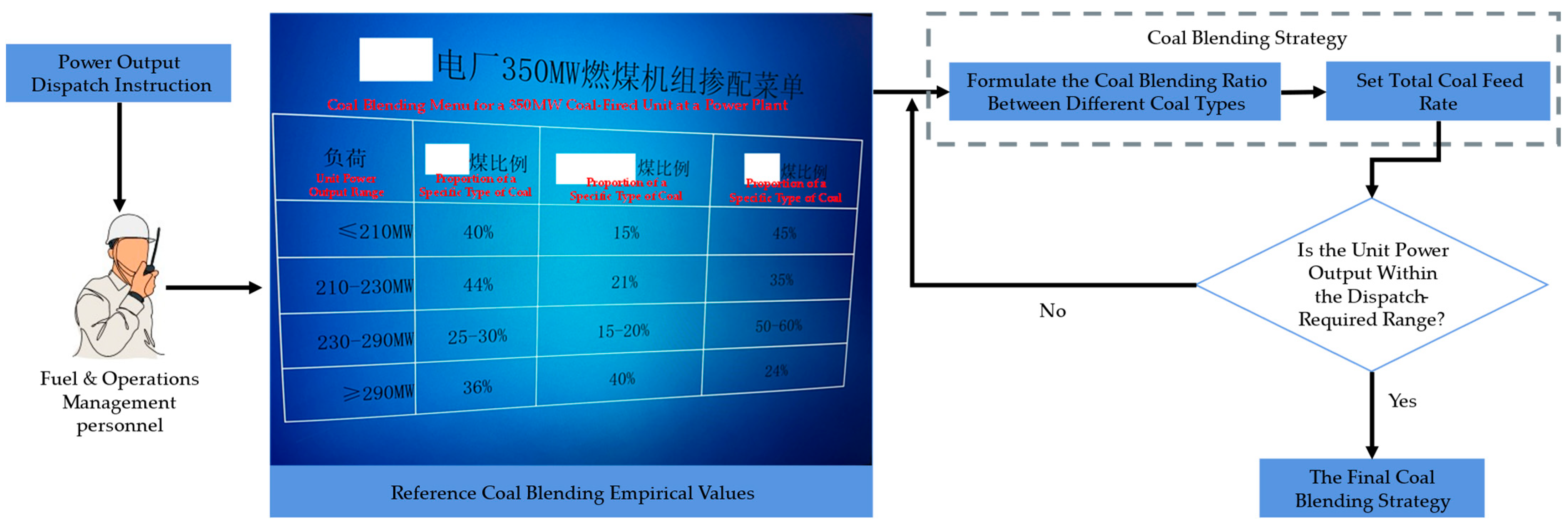
2. Coal Blending Decision-Making for Thermal Power Units
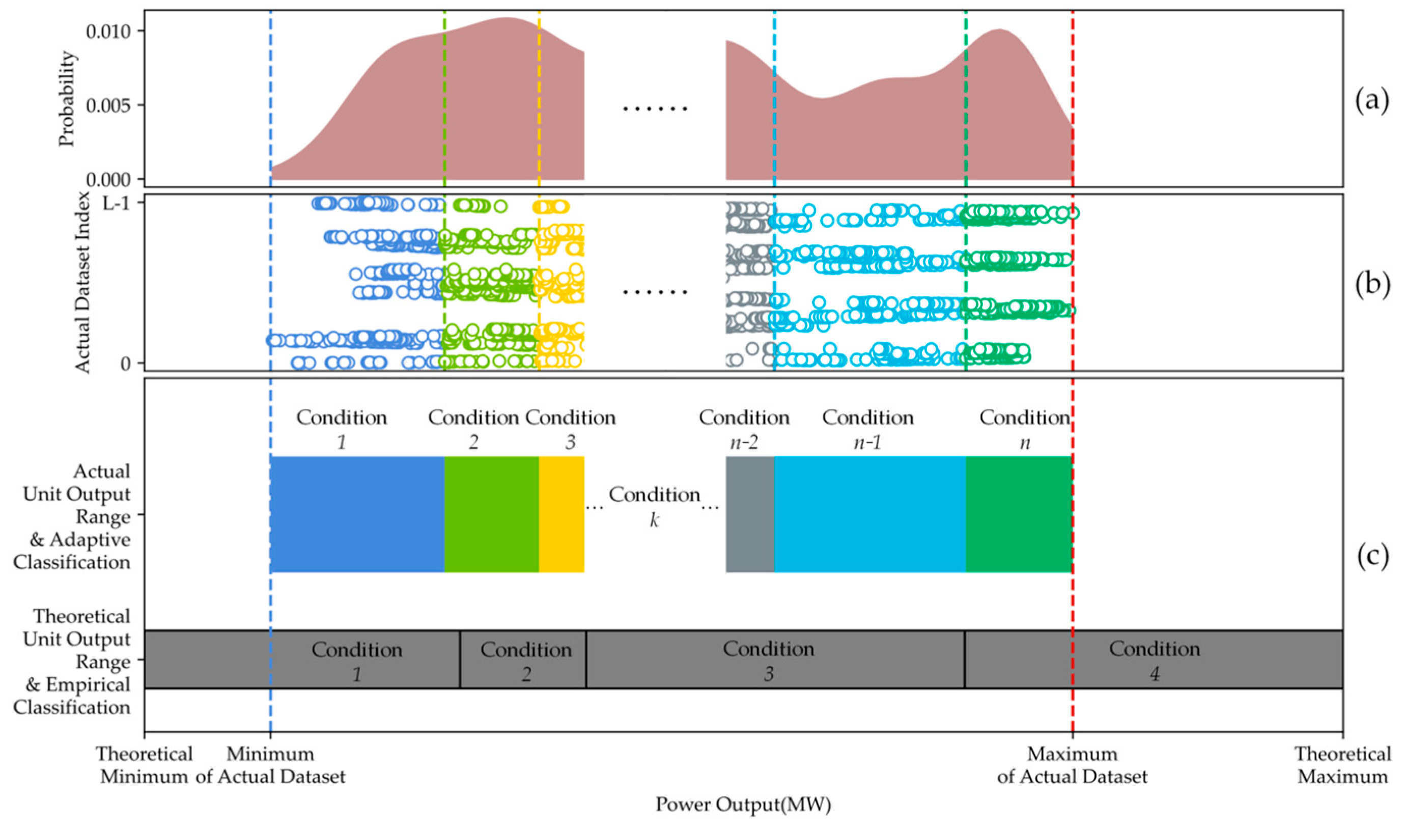
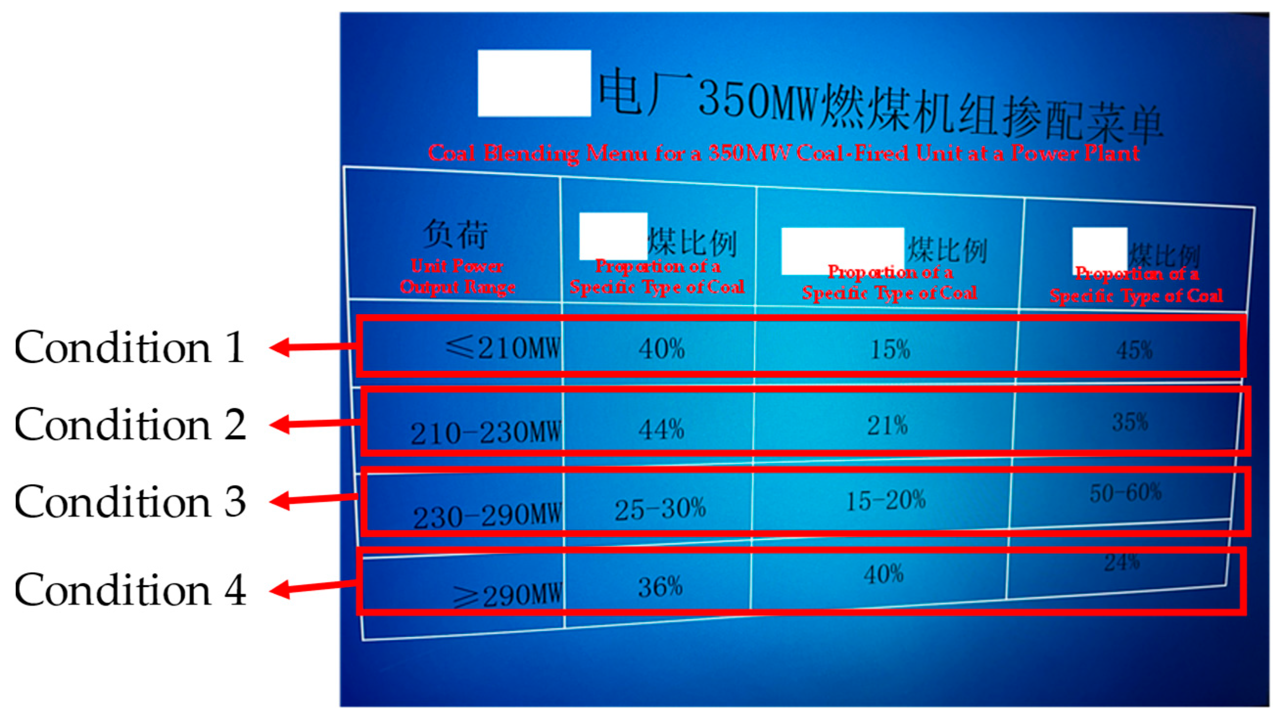
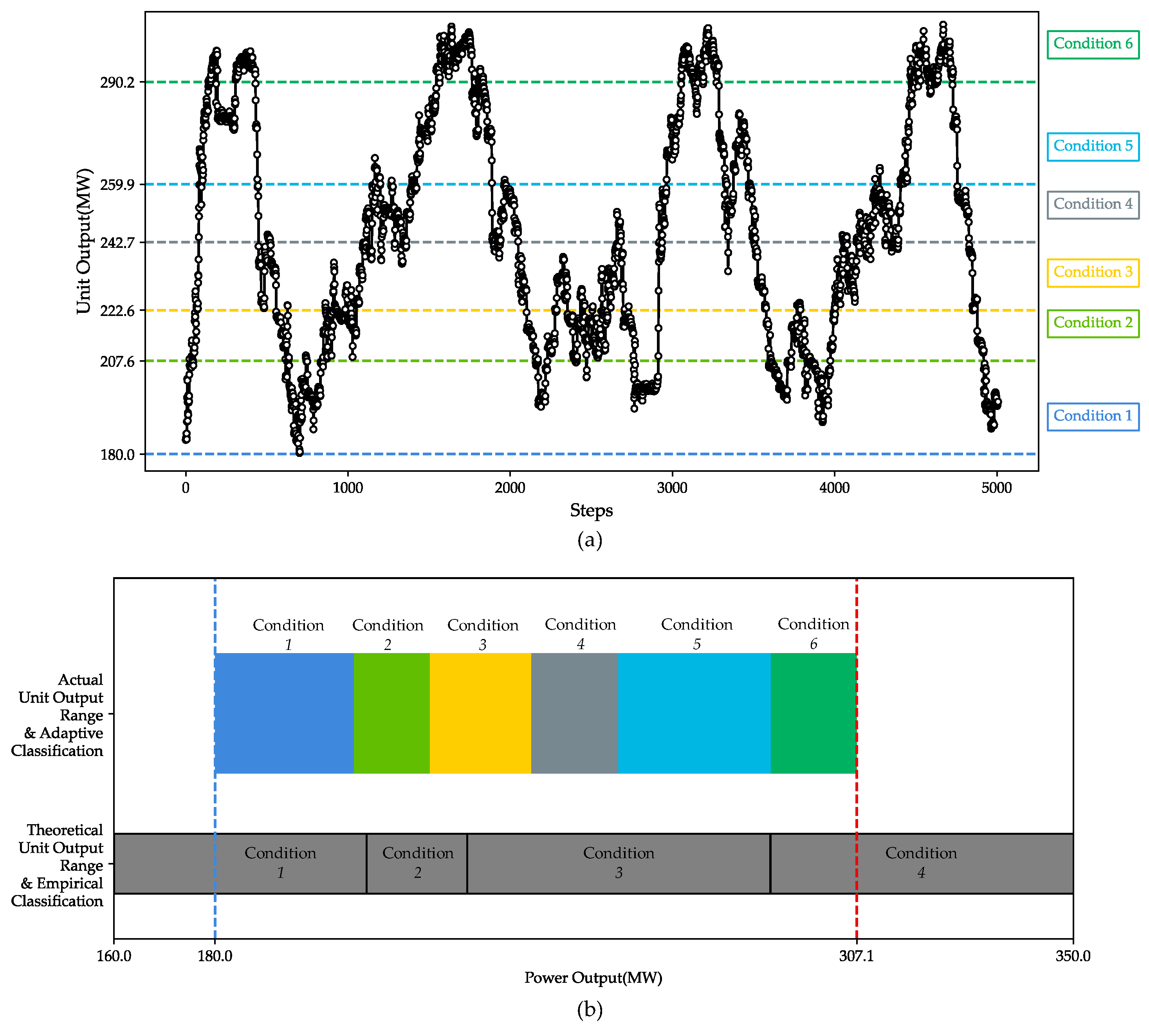
- The output condition classification that serves as a reference for initial CBS may not adapt well to actual circumstances. This decision-making process provides fixed condition classifications based on theoretical output limits and derives an initial CBS from past experience. However, during operation, the grid’s dispatch of unit output adjusts according to the actual power load, with outputs often concentrated within a specific range of the theoretical limits. This range may be covered by only a minimal number of reference condition classifications, resulting in an initial CBS with insufficient granularity that lacks the adaptability to adjust dynamically to real production needs, thus differing significantly from the final feasible CBS. Additionally, the initial CBS primarily focuses on coal cost, to some extent overlooking other cost types.
- The method of adjusting the initial CBS to form the final CBS is inefficient and fails to ensure economic viability. The process of fine-tuning the initial CBS to a final CBS relies entirely on continuous adjustments based on actual output feedback and manual judgment. This process may lead to fuel wastage and has a high probability of compromising the economic efficiency of the initial blending strategy.
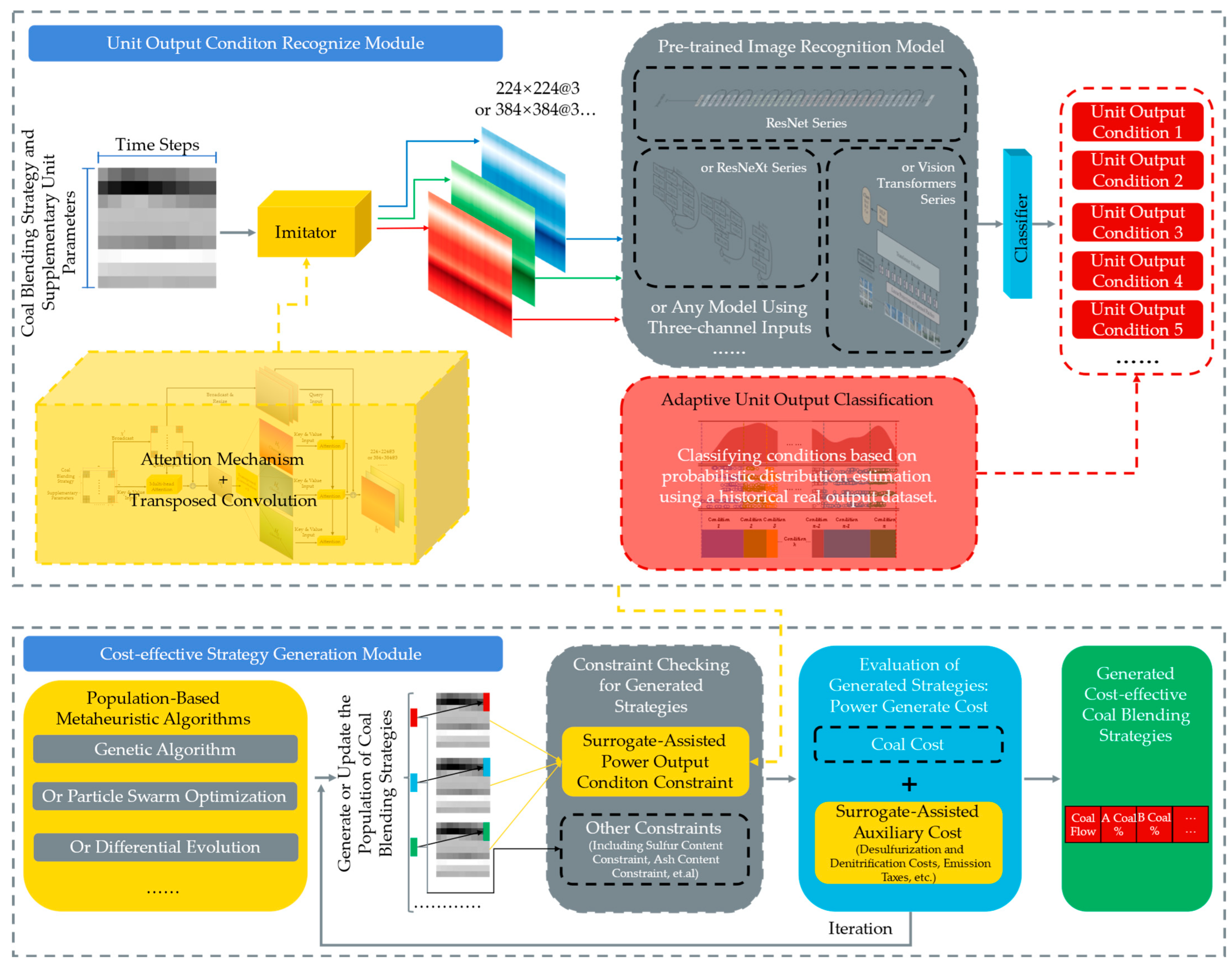
3. Framework for Generating Cost-Effective Coal Blending Strategy
3.1. Unit Output Condition Recognition Module
3.1.1. Adaptive Unit Output Condition Classification
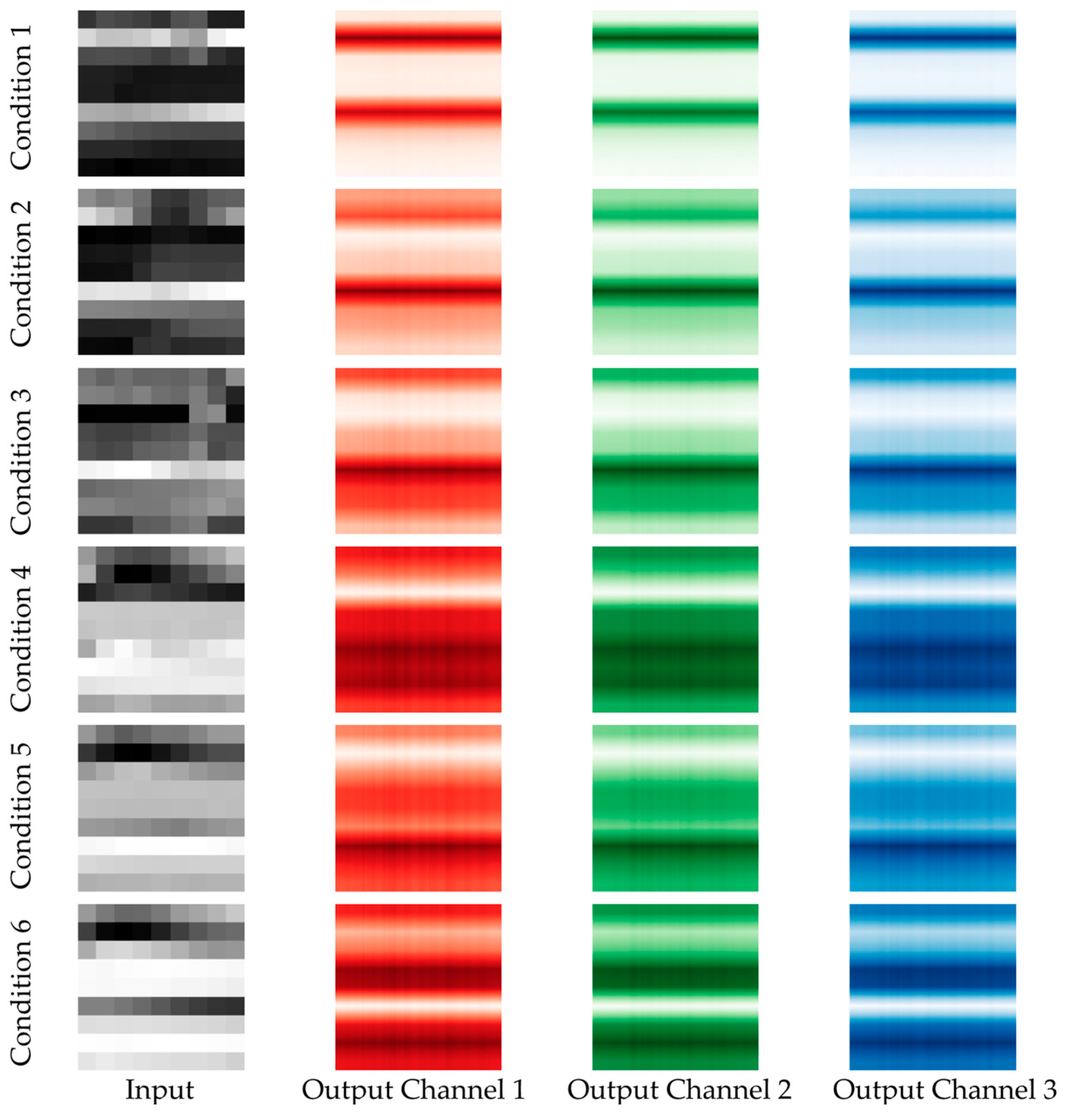
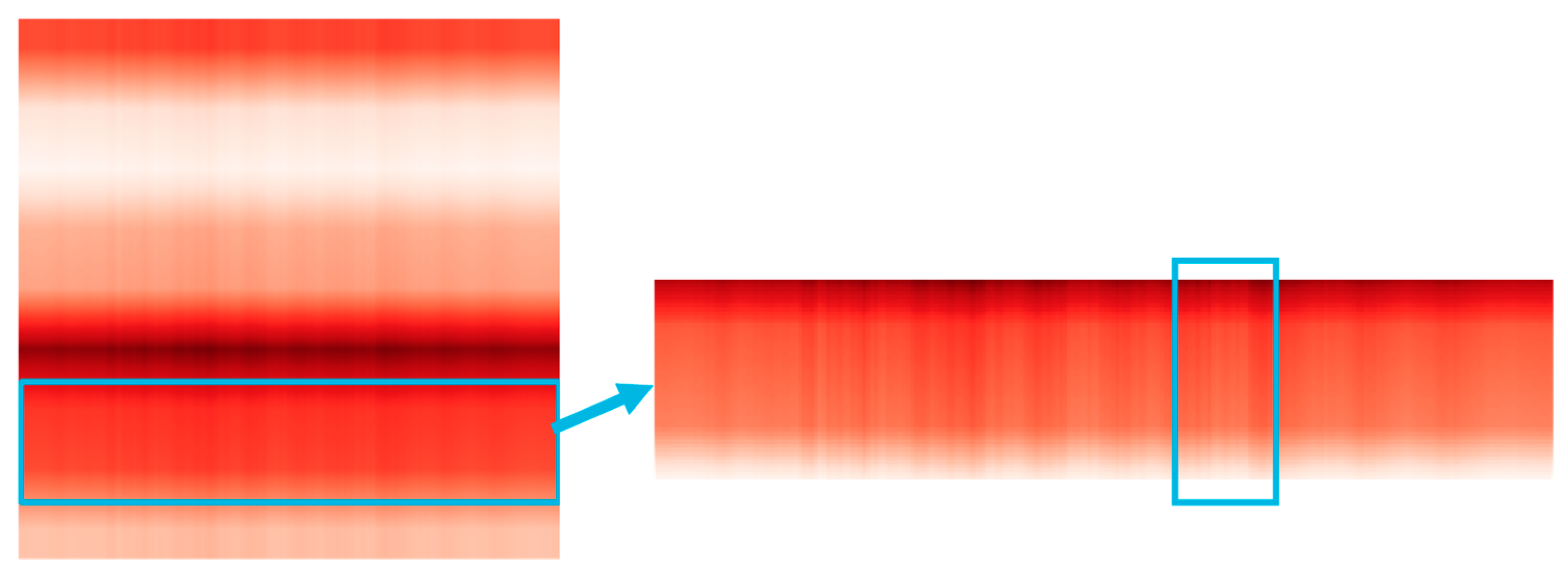
3.1.2. Imitator
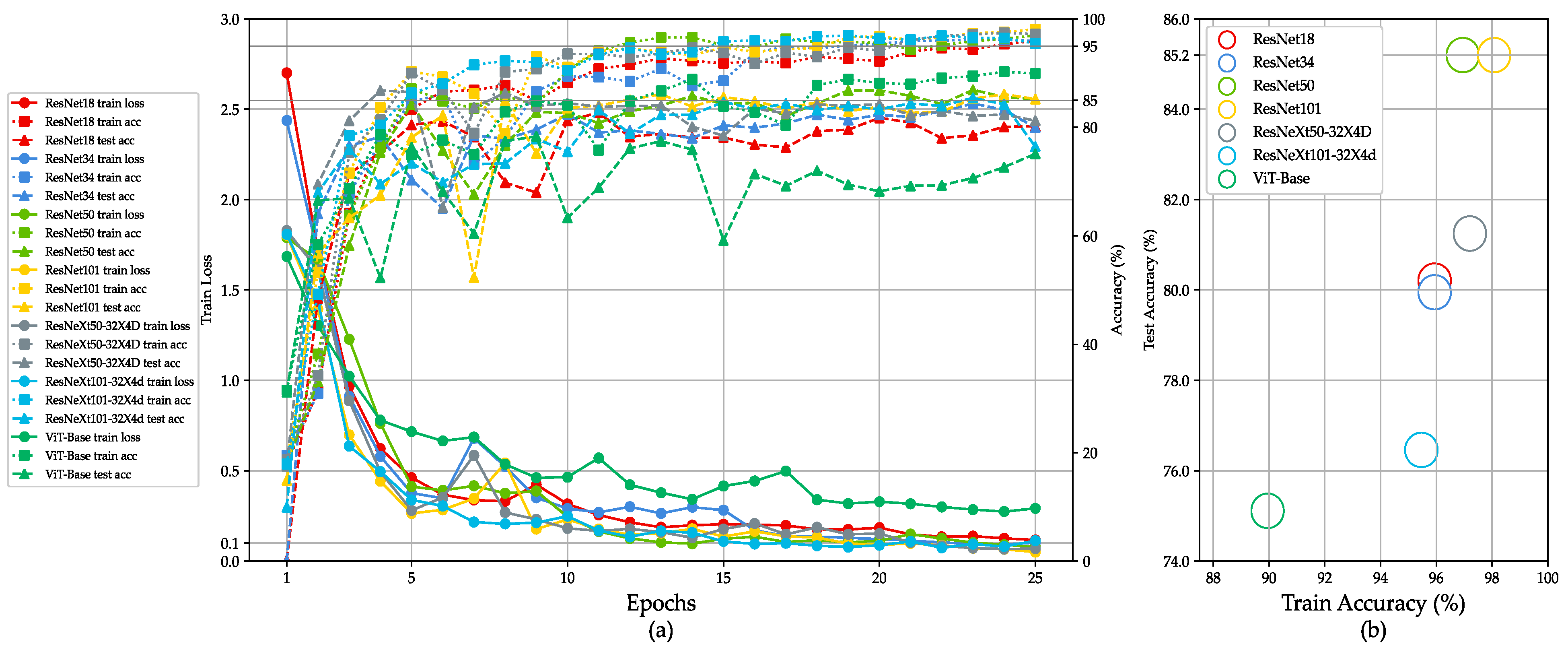
3.1.3. Intelligent Condition Recognition Based on Pre-Trained Image Classification Models
3.2. Cost-Effective Strategy Generation Module
3.2.1. Calculation of Power Generation Costs and Coal Quality Indicators
3.2.2. Surrogate-Assisted Generation Model
3.2.3. Cost-Effective CBS Generation
| Algorithm 1. The Pseudocode for the CBS Generation Process of CESG | |||||
| Input , , | |||||
| Output , | |||||
| Initialize , , | |||||
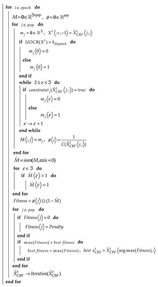 | |||||
| return , |
4. Case Study and Analysis
4.1. Overview of the Sample Coal-Fired Unit and Experimental Environment
4.2. Sample Dataset
4.3. Hyperparameter Settings for Proposed Framework
4.4. Experimental Results and Analysis of UOCR
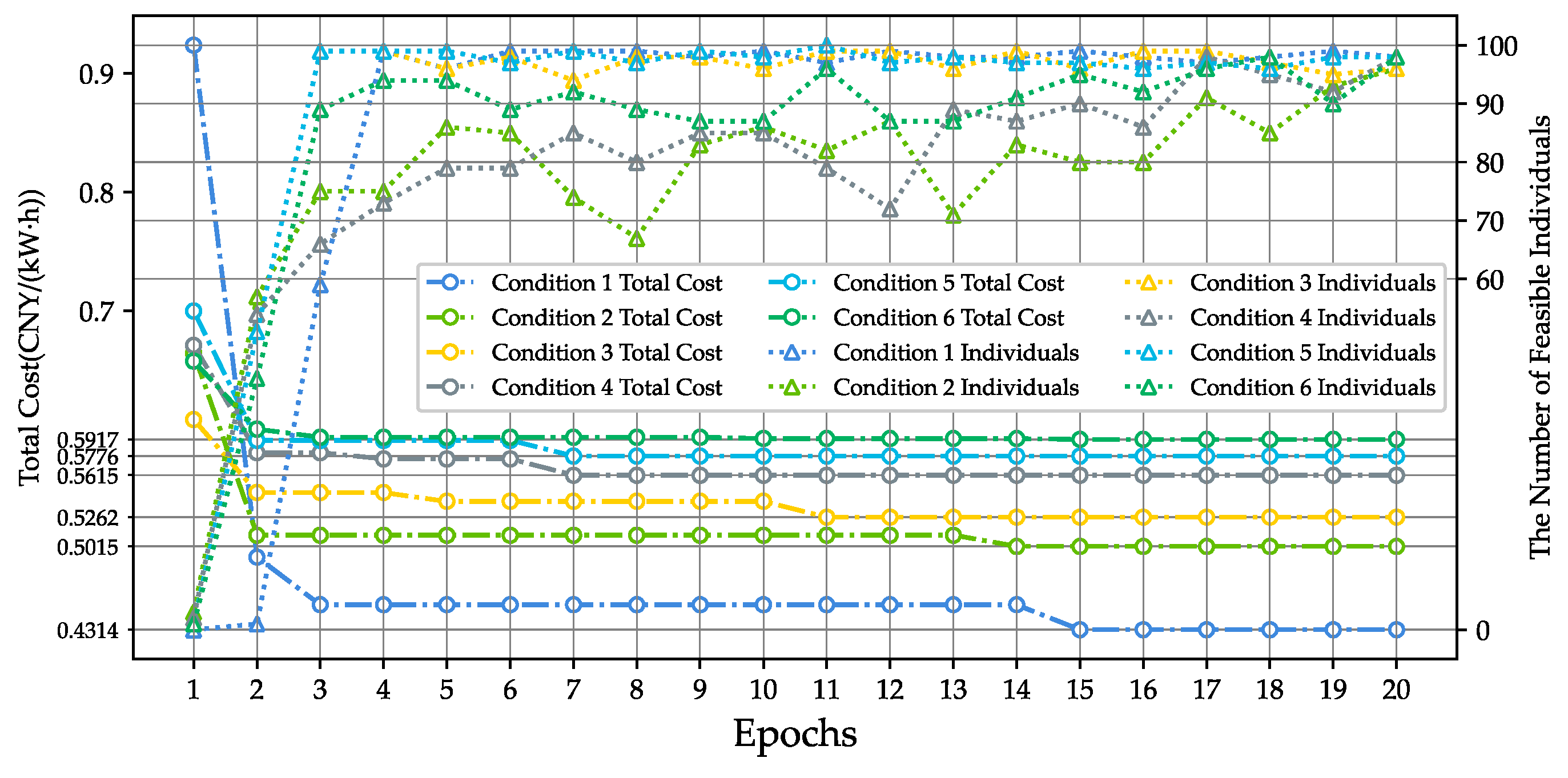
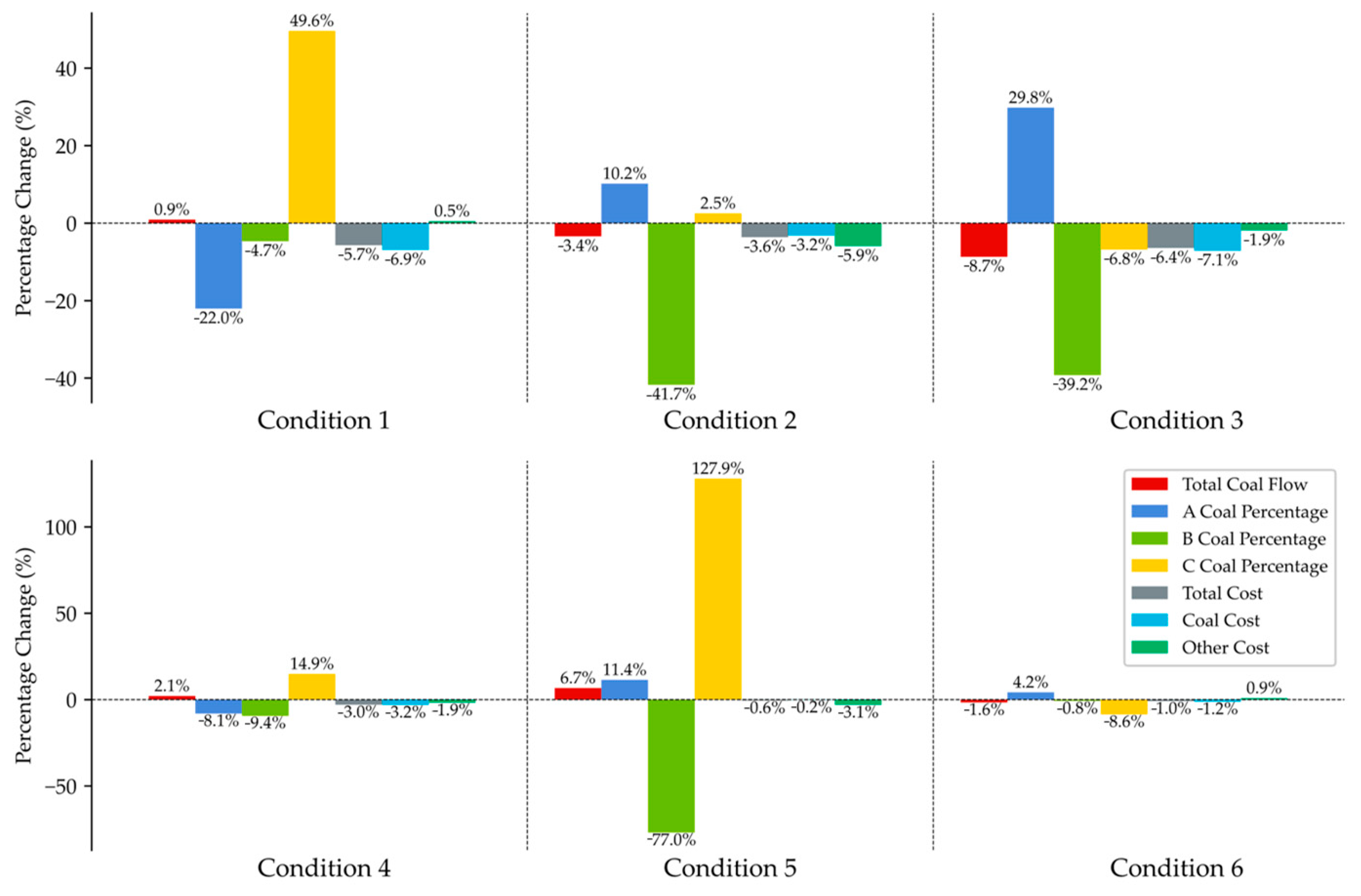
4.5. Experimental Results and Analysis of CESG
5. Discussion
- The design concept of combining the Imitator with pre-trained image classification models in the UOCR module offers promising opportunities for applying larger-scale deep learning models to the thermal power sector. This approach provides a potential pathway for leveraging advanced model architectures with greater parameter capacity in industrial applications.
- Conducting more extensive case studies is necessary to comprehensively evaluate the framework’s design. Different types of thermal power units, such as ultra-supercritical units or those combined with renewable energy generation, operate under distinct mechanisms, which may pose new challenges to the framework’s stability. Additionally, thermal power units in different regions face varying cost structures, requiring adjustments to auxiliary cost design based on case studies. For instance, European thermal power plants may need to incorporate carbon footprint considerations into cost calculations.
- The framework’s performance in engineering environments requires further experimentation. In the current case study, the trained framework took 50–70 seconds from initialization to generating a cost-effective CBS (detailed timing information is provided in the Figure 3), leaving room for improvement. However, the experimental environment in this study may not represent the operational conditions available in most engineering applications. The framework needs to be tested in a wider range of operating environments to comprehensively validate its performance.
6. Conclusions
Author Contributions
Funding
Data Availability Statement
Conflicts of Interest
References
- National Bureau of Statistics of China. Statistical Communiqué of the People’s Republic of China on the 2023 National Economic and Social Development. Available online: https://www.stats.gov.cn/english/PressRelease/202402/t20240228_1947918.html (accessed on 2 November 2024).
- Srinivasan, P.; Shekhar, A. Internalizing the External Cost of Gaseous and Particulate Matter Emissions from the Coal-Based Thermal Power Plants in India. Part. Sci. Technol. 2021, 39, 632–640. [Google Scholar] [CrossRef]
- Xie, S.; Qin, P.; Zhang, M.; Xu, J.; Ouyang, T. A High-Efficiency and Eco-Friendly Design for Coal-Fired Power Plants: Combined Waste Heat Recovery and Electron Beam Irradiation. Energy 2022, 258, 124884. [Google Scholar] [CrossRef]
- Yuan, X.; Chen, L.; Sheng, X.; Liu, M.; Xu, Y.; Tang, Y.; Wang, Q.; Ma, Q.; Zuo, J. Life Cycle Cost of Electricity Production: A Comparative Study of Coal-Fired, Biomass, and Wind Power in China. Energies 2021, 14, 3463. [Google Scholar] [CrossRef]
- Lin, L.; Xu, B.; Xia, S. Multi-Angle Economic Analysis of Coal-Fired Units with Plasma Ignition and Oil Injection during Deep Peak Shaving in China. Appl. Sci. 2019, 9, 5399. [Google Scholar] [CrossRef]
- Ali, H.; Phoumin, H.; Weller, S.R.; Suryadi, B. Cost–Benefit Analysis of HELE and Subcritical Coal-Fired Electricity Generation Technologies in Southeast Asia. Sustainability 2021, 13, 1591. [Google Scholar] [CrossRef]
- Zhao, B.; Chen, G.; Qin, L.; Han, Y.; Zhang, Q.; Chen, W.; Han, J. Effect of Coal Blending on Arsenic and Fine Particles Emission during Coal Combustion. J. Clean. Prod. 2021, 311, 127645. [Google Scholar] [CrossRef]
- Baek, S.H.; Park, H.Y.; Ko, S.H. The Effect of the Coal Blending Method in a Coal Fired Boiler on Carbon in Ash and NOx Emission. Fuel 2014, 128, 62–70. [Google Scholar] [CrossRef]
- Khabarova, M.A.; Novikova, O.V.; Khabarov, A.A. State and Perspectives of Power and Industry Applications of Coal. In Proceedings of the 2019 IEEE Conference of Russian Young Researchers in Electrical and Electronic Engineering (EIConRus), St. Petersburg, Russia, 28–31 January 2019; pp. 985–987. [Google Scholar]
- Wang, Y.; Liu, Z.; Huang, H.; Xiong, X. Reducing Measurement Costs of Thermal Power: An Advanced MISM (Mamba with Improved SSM Embedding in MLP) Regression Model for Accurate CO2 Emission Accounting. Sensors 2024, 24, 6256. [Google Scholar] [CrossRef] [PubMed]
- Wu, Y.; Ke, Y.; Xu, C.; Xiao, X.; Hu, Y. Eco-Efficiency Measurement of Coal-Fired Power Plants in China Using Super Efficiency Data Envelopment Analysis. Sustain. Cities Soc. 2018, 36, 157–168. [Google Scholar] [CrossRef]
- Zaid, M.Z.S.M.; Wahid, M.A.; Mailah, M.; Mazlan, M.A.; Saat, A. Coal Fired Power Plant: A Review on Coal Blending and Emission Issues. AIP Conf. Proc. 2019, 2062, 020022. [Google Scholar] [CrossRef]
- Yan, S.; Lv, C.; Yao, L.; Hu, Z.; Wang, F. Hybrid Dynamic Coal Blending Method to Address Multiple Environmental Objectives under a Carbon Emissions Allocation Mechanism. Energy 2022, 254, 124297. [Google Scholar] [CrossRef]
- Lv, C.; Xu, J.; Xie, H.; Zeng, Z.; Wu, Y. Equilibrium Strategy Based Coal Blending Method for Combined Carbon and PM10 Emissions Reductions. Appl. Energy 2016, 183, 1035–1052. [Google Scholar] [CrossRef]
- Amini, S.H.; Vass, C.; Shahabi, M.; Noble, A. Optimization of Coal Blending Operations under Uncertainty—Robust Optimization Approach. Int. J. Coal Prep. Util. 2022, 42, 30–50. [Google Scholar] [CrossRef]
- Yuan, Y.; Qu, Q.; Chen, L.; Wu, M. Modeling and Optimization of Coal Blending and Coking Costs Using Coal Petrography. Inf. Sci. 2020, 522, 49–68. [Google Scholar] [CrossRef]
- Nawaz, Z.; Ali, U. Techno-Economic Evaluation of Different Operating Scenarios for Indigenous and Imported Coal Blends and Biomass Co-Firing on Supercritical Coal Fired Power Plant Performance. Energy 2020, 212, 118721. [Google Scholar] [CrossRef]
- Huang, S.; Xiong, L.; Zhou, Y.; Gao, F.; Jia, Q.; Li, X.; Li, X.; Wang, Z.; Khan, M.W. Robust Distributed Fixed-Time Fault-Tolerant Control for Shipboard Microgrids With Actuator Fault. IEEE Trans. Transp. Electrif. 2024. [Google Scholar] [CrossRef]
- Huang, C.; Li, Z. Data-Driven Modeling of Ultra-Supercritical Unit Coordinated Control System by Improved Transformer Network. Energy 2023, 266, 126473. [Google Scholar] [CrossRef]
- Huang, C.; Sheng, X. Data-Driven Model Identification of Boiler-Turbine Coupled Process in 1000 MW Ultra-Supercritical Unit by Improved Bird Swarm Algorithm. Energy 2020, 205, 118009. [Google Scholar] [CrossRef]
- He, K.; Zhang, X.; Ren, S.; Sun, J. Deep Residual Learning for Image Recognition. In Proceedings of the 2016 IEEE Conference on Computer Vision and Pattern Recognition (CVPR), Las Vegas, NV, USA, 27–30 June 2016; pp. 770–778. [Google Scholar]
- Xie, S.; Girshick, R.; Dollar, P.; Tu, Z.; He, K. Aggregated Residual Transformations for Deep Neural Networks. In Proceedings of the 2017 IEEE Conference on Computer Vision and Pattern Recognition (CVPR), Honolulu, HI, USA, 21–26 July 2017; pp. 5987–5995. [Google Scholar]
- Dosovitskiy, A.; Beyer, L.; Kolesnikov, A.; Weissenborn, D.; Zhai, X.; Unterthiner, T.; Dehghani, M.; Minderer, M.; Heigold, G.; Gelly, S.; et al. An Image Is Worth 16x16 Words: Transformers for Image Recognition at Scale. arXiv 2020, arXiv:2010.11929. [Google Scholar]
- Models and Pre-Trained Weights—Torchvision 0.20 Documentation. Available online: https://pytorch.org/vision/stable/models.html (accessed on 27 October 2024).
- Google/Vit-Base-Patch16-384·Hugging Face. Available online: https://huggingface.co/google/vit-base-patch16-384 (accessed on 27 October 2024).
- Ke, G.; Meng, Q.; Finley, T.; Wang, T.; Chen, W.; Ma, W.; Ye, Q.; Liu, T.-Y. LightGBM: A Highly Efficient Gradient Boosting Decision Tree. Adv. Neural Inf. Process. Syst. 2017, 30. [Google Scholar]
- Prokhorenkova, L.; Gusev, G.; Vorobev, A.; Dorogush, A.V.; Gulin, A. CatBoost: Unbiased Boosting with Categorical Features. In Proceedings of the 32nd International Conference on Neural Information Processing Systems, Montreal, QC, Canada, 3–8 December 2018; Curran Associates Inc.: Red Hook, NY, USA, 2018; pp. 6639–6649. [Google Scholar]
- Geurts, P.; Ernst, D.; Wehenkel, L. Extremely Randomized Trees. Mach. Learn. 2006, 63, 3–42. [Google Scholar] [CrossRef]
- Cover, T.; Hart, P. Nearest Neighbor Pattern Classification. IEEE Trans. Inf. Theor. 2006, 13, 21–27. [Google Scholar] [CrossRef]
- Paszke, A.; Gross, S.; Chintala, S.; Chanan, G.; Yang, E.; DeVito, Z.; Lin, Z.; Desmaison, A.; Antiga, L.; Lerer, A. Automatic Differentiation in PyTorch. 28 October 2017.
- Breiman, L. Random Forests. Mach. Learn. 2001, 45, 5–32. [Google Scholar] [CrossRef]
- Chen, T.; Guestrin, C. XGBoost: A Scalable Tree Boosting System. In Proceedings of the 22nd ACM SIGKDD International Conference on Knowledge Discovery and Data Mining, San Francisco, CA, USA, 13–17 August 2016; Association for Computing Machinery: New York, NY, USA, 2016; pp. 785–794. [Google Scholar]
- Howard, J.; Gugger, S. Fastai: A Layered API for Deep Learning. Information 2020, 11, 108. [Google Scholar] [CrossRef]
- Zhou, Z.-H. Ensemble Methods: Foundations and Algorithms, 1st ed.; Chapman & Hall/CRC: Boca Raton, FL, USA, 2012; ISBN 978-1-4398-3003-1. [Google Scholar]
- Improved Roulette Wheel Selection-Based Genetic Algorithm for TSP|IEEE Conference Publication|IEEE Xplore. Available online: https://ieeexplore.ieee.org/document/7945968 (accessed on 27 October 2024).
- Wu, S.; Wang, H.; Yu, W.; Yang, K.; Cao, D.; Wang, F. A New SOTIF Scenario Hierarchy and Its Critical Test Case Generation Based on Potential Risk Assessment. In Proceedings of the 2021 IEEE 1st International Conference on Digital Twins and Parallel Intelligence (DTPI), Beijing, China, 15 July–15 August 2021; pp. 399–409. [Google Scholar] [CrossRef]
- Li, Y.; Wu, S.; Wang, H. Adaptive Mining of Failure Scenarios for Autonomous Driving Systems Based on Multi-Population Genetic Algorithm. In Proceedings of the 2024 IEEE Intelligent Vehicles Symposium (IV), Jeju Island, Republic of Korea, 2–5 June 2024; pp. 2458–2464. [Google Scholar]


| Mean | Min | Max | |
|---|---|---|---|
| Total Coal Flow Rate (t/h) | 145.38 | 72.03 | 240.85 |
| A Coal Percentage (%) | 0.41 | 0.21 | 0.75 |
| B Coal Percentage (%) | 0.27 | 0.07 | 0.61 |
| Main Steam Pressure (MPa) | 2.70 | 1.92 | 3.47 |
| Main Steam Flow Rate (t/h) | 785.83 | 534.33 | 1038.70 |
| Main Steam Temperature (°C) | 567.21 | 547.52 | 581.52 |
| Feedwater Pressure (MPa) | 22.09 | 16.00 | 26.38 |
| Feedwater Temperature (°C) | 269.27 | 251.43 | 283.59 |
| Feedwater Flow Rate (t/h) | 772.52 | 540.43 | 1042.08 |
| Quality Indicators | Coal Type | ||
|---|---|---|---|
| A | B | C | |
| Sulfur Content (%) | 1.17 | 1.22 | 1.26 |
| Ash Content (%) | 29.26 | 28.63 | 30.79 |
| Volatile Matter (%) | 17.42 | 15.90 | 16.33 |
| Calorific Value (Kcal/kg) | 5200.00 | 4576.81 | 3205.24 |
| Price (CNY/t) | 843.31 | 725.77 | 650.28 |
| Power Output Situation Label Number | Input Steps length | Train Hyperparameter | |||
|---|---|---|---|---|---|
| Epoch | Initial Learning Rate of Imitator | Initial Learning Rate of Pre-Trained Model | Initial Learning Rate of Classifier | ||
| 6 | 9 | 25 | 1 × 10⁻⁴ | 1 × 10⁻⁵ | 1 × 10⁻⁴ |
| Number of Parameters | Source of Pre-Trained Weights | Batch Size | |
|---|---|---|---|
| ResNet18 | 11.7M | [24] | 256 |
| ResNet34 | 21.8M | 256 | |
| ResNet50 | 25.6M | 200 | |
| ResNet101 | 44.5M | 100 | |
| ResNeXt50-32X4D | 25.0M | 128 | |
| ResNeXt101-32X4D | 88.8M | 64 | |
| Vit-Base | 86.4M | [25] | 64 |
| Minimum | Maximum | |
|---|---|---|
| Sulfur Content (%) | - | 1.5 |
| Ash Content (%) | - | 30 |
| Volatile Matter (%) | - | 20 |
| Calorific Value (Kcal/kg) | 4200 |
| Population Size | Crossover Rate | Mutation Rate | Max Generations |
|---|---|---|---|
| 100 | 0.80 | 0.01 | 20 |
| Training Loss | Training Accuracy | Test Accuracy | |
|---|---|---|---|
| ResNet18 | 1.164 × 10⁻¹ | 95.94% | 80.21% |
| ResNet34 | 1.024 × 10⁻¹ | 95.94% | 79.95% |
| ResNet50 | 7.723 × 10⁻² | 96.95% | 85.20% |
| ResNet101 | 4.925 × 10⁻² | 98.08% | 85.20% |
| ResNeXt50-32X4D | 6.914 × 10⁻² | 97.20% | 81.25% |
| ResNeXt101-32X4D | 1.129 × 10⁻¹ | 95.46% | 76.46% |
| ViT-Base | 2.914 × 10⁻¹ | 89.94% | 75.11% |
| Train RMSE | Test RMSE | Test MAPE | |
|---|---|---|---|
| WeightedEnsemble | 1.625 × 10⁻³ | 3.706 × 10⁻³ | 4.312% |
| LightGBMXT | 1.694 × 10⁻³ | 3.800 × 10⁻³ | 4.428% |
| CatBoost | 1.706 × 10⁻³ | 3.728 × 10⁻³ | 4.386% |
| LightGBM | 1.708 × 10⁻³ | 3.776 × 10⁻³ | 4.356% |
| LightGBMLarge | 1.780 × 10⁻³ | 3.678 × 10⁻³ | 4.277% |
| ExtraTrees | 1.812 × 10⁻³ | 3.416 × 10⁻³ | 3.990% |
| KneighborsDist | 1.857 × 10⁻³ | 4.080 × 10⁻³ | 4.683% |
| NeuralNetTorch | 1.927 × 10⁻³ | 3.855 × 10⁻³ | 4.324% |
| RandomForest | 1.937 × 10⁻³ | 3.643 × 10⁻³ | 4.246% |
| KneighborsUnif | 1.970 × 10⁻³ | 4.066 × 10⁻³ | 4.663% |
| XGBoost | 2.006 × 10⁻³ | 3.563 × 10⁻³ | 4.173% |
| NeuralNetFastAI | 2.348 × 10⁻³ | 3.338 × 10⁻³ | 3.831% |
| Total Coal Flow Rate (t/h) | A Coal Percentage | B Coal Percentage | Total Cost (CNY/ (kW·h)) | Coal Cost (CNY/ (kW·h)) | Other Cost (CNY/ (kW·h)) | |
|---|---|---|---|---|---|---|
| Cond. 1 Orig. | 88.803 | 59.53% | 12.82% | 0.457 | 0.382 | 0.075 |
| Cond. 1 Gen. | 89.620 | 46.41% | 12.23% | 0.431 | 0.356 | 0.075 |
| Cond. 2 Orig. | 122.521 | 44.47% | 13.43% | 0.520 | 0.440 | 0.080 |
| Cond. 2 Gen. | 118.318 | 49.01% | 7.83% | 0.501 | 0.426 | 0.075 |
| Cond. 3 Orig. | 147.906 | 35.48% | 19.04% | 0.562 | 0.487 | 0.075 |
| Cond. 3 Gen. | 135.080 | 46.05% | 11.57% | 0.526 | 0.452 | 0.074 |
| Cond. 4 Orig. | 164.573 | 44.22% | 19.42% | 0.579 | 0.509 | 0.070 |
| Cond. 4 Gen. | 168.005 | 40.64% | 17.60% | 0.561 | 0.493 | 0.069 |
| Cond. 5 Orig. | 174.444 | 43.09% | 37.92% | 0.581 | 0.512 | 0.069 |
| Cond. 5 Gen. | 186.077 | 48.02% | 8.71% | 0.578 | 0.511 | 0.067 |
| Cond. 6 Orig. | 200.385 | 43.91% | 38.05% | 0.597 | 0.527 | 0.070 |
| Cond. 6 Gen. | 197.129 | 45.76% | 37.75% | 0.592 | 0.521 | 0.071 |
Disclaimer/Publisher’s Note: The statements, opinions and data contained in all publications are solely those of the individual author(s) and contributor(s) and not of MDPI and/or the editor(s). MDPI and/or the editor(s) disclaim responsibility for any injury to people or property resulting from any ideas, methods, instructions or products referred to in the content. |
© 2025 by the authors. Licensee MDPI, Basel, Switzerland. This article is an open access article distributed under the terms and conditions of the Creative Commons Attribution (CC BY) license (https://creativecommons.org/licenses/by/4.0/).
Share and Cite
Wang, X.; Wu, S.; Wang, T.; Ding, J. A Surrogate-Assisted Intelligent Adaptive Generation Framework for Cost-Effective Coal Blending Strategy in Thermal Power Units. Electronics 2025, 14, 561. https://doi.org/10.3390/electronics14030561
Wang X, Wu S, Wang T, Ding J. A Surrogate-Assisted Intelligent Adaptive Generation Framework for Cost-Effective Coal Blending Strategy in Thermal Power Units. Electronics. 2025; 14(3):561. https://doi.org/10.3390/electronics14030561
Chicago/Turabian StyleWang, Xiang, Siyu Wu, Teng Wang, and Jiangrui Ding. 2025. "A Surrogate-Assisted Intelligent Adaptive Generation Framework for Cost-Effective Coal Blending Strategy in Thermal Power Units" Electronics 14, no. 3: 561. https://doi.org/10.3390/electronics14030561
APA StyleWang, X., Wu, S., Wang, T., & Ding, J. (2025). A Surrogate-Assisted Intelligent Adaptive Generation Framework for Cost-Effective Coal Blending Strategy in Thermal Power Units. Electronics, 14(3), 561. https://doi.org/10.3390/electronics14030561