Abstract
This study explores a hybrid forecasting framework for air pollutant concentrations (PM10, PM2.5, and NO2) that integrates Seasonal Autoregressive Integrated Moving Average (SARIMA) models with Bidirectional Long Short-Term Memory (BiLSTM) networks. By leveraging SARIMA’s strength in linear and seasonal trend modeling and addressing nonlinear dependencies using BiLSTM, the framework incorporates Box-Cox transformations and Fourier terms to enhance variance stabilization and seasonal representation. Additionally, attention mechanisms are employed to prioritize temporal features, refining forecast accuracy. Using five years of daily pollutant data from Romania’s National Air Quality Monitoring Network, the models were rigorously evaluated across short-term (1-day), medium-term (7-day), and long-term (30-day) horizons. Metrics such as RMSE, MAE, and MAPE revealed the hybrid models’ superior performance in capturing complex pollutant dynamics, particularly for PM2.5 and PM10. The SARIMA combined with BiLSTM, Fourier, and Attention configuration demonstrated consistent improvements in predictive accuracy and interpretability, with attention mechanisms proving effective for extreme values and long-term dependencies. This study highlights the benefits of combining statistical preprocessing with advanced neural architectures, offering a robust and scalable solution for air quality forecasting. The findings provide valuable insights for environmental policymakers and urban planners, emphasizing the potential of hybrid models for improving air quality management and decision-making in dynamic urban environments.
Keywords:
air pollution; SARIMA; BiLSTM; fourier terms; attention mechanisms; forecasting; hybrid models 1. Introduction
Air pollution remains one of the most critical environmental challenges of our time, affecting public health and quality of life worldwide. Despite improvements in air quality over the decades, urban populations continue to face significant risks from particulate matter and other pollutants. The modern cultural preoccupation with nature, clean air, and quality of life often arises from health-related anxieties. Eugène Ionesco’s statement, ’In the countryside, the air is cleaner because the peasants sleep with the windows closed’, humorously illustrates the oversimplifications often made when addressing complex issues like air quality. This irony invites a deeper exploration of air pollution levels and the patterns underlying them—not just as a scientific inquiry, but as a societal necessity to safeguard public health. Air quality is shaped by both natural variability and human activities, which interact in complex ways that require integrated analysis. Despite improvements in air quality over the decades, air pollution remains a significant health hazard. According to the European Environment Agency (2024) [1], poor air quality contributes to 300,000 premature deaths annually in Europe, with 96% of urban residents exposed to unsafe PM2.5 concentrations.
Given that air pollution adversely affects individuals of all ages and produces emerging phenomena with uncertain long-term impacts, it is crucial to prioritize strategies for adaptation and mitigation to ensure a sustainable future. A recent study by George Washington University [2], published in The Lancet Planetary Health, analyzed data from over 13,000 cities over the past two decades. The findings reveal a critical risk: 86% of urban residents worldwide—around 2.5 billion people—are exposed to pollution levels nearly seven times higher than WHO recommendations. In 2021, WHO revised its air quality guidelines to address the ongoing and significant threat of air pollution to public health [3]. Their experts decided on which pollutants to update, including particulate matter, ozone, nitrogen dioxide, and sulphur dioxide. PM, O3, NO2, and SO2 are considered common air pollutants. According to Southerland et al. (2022) [2], urban air pollution at these levels contributed to approximately 1.8 million deaths in 2019, largely due to fine particles (PM2.5) under 2.5 microns in diameter, which remain suspended in the air as inhalable solid particles or microscopic liquid droplets. The issue is particularly critical in densely populated urban areas where industrial emissions, vehicle exhaust, and other pollutants converge, posing acute risks to vulnerable populations, including children, the elderly, and individuals with pre-existing health conditions.
Despite ongoing overall improvements in air quality, current EU standards are still not met in Romania. The WHO [3] recommended a maximum level of particulate matter (PM2.5) of 5 micrograms per cubic meter to avoid putting our health and lives at risk. The 2024 ranking of Europe’s urban agglomerations shows that Romania has no city with good air quality that falls within this limit. With 15.7 micrograms of PM2.5 per cubic meter, Bucharest ranks 314 out of 372, making it one of the most polluted cities in Romania, according to European Environment Agency data [4]. Bucharest falls into the “poor” air quality category, with values ranging from 15 to 25 micrograms per cubic meter.
Bucharest, ranked 9th among the top 96 European cities, faces persistent health risks from air pollution, partly attributed to its ongoing urban expansion. The most important source of pollution for Bucharest and its surrounding area is combustion. According to the sensor values, cooler weather brings an increase in pollution levels. The index map is red in the cold season because of heating with central heating plants and stoves, a problem that has persisted for years. Another significant factor is the intensity of traffic during rush hours. According to Airly [5], during the evening peak, average PM10 concentrations are approximately 25% higher compared to midday levels. In the summer of 2024, the lack of rainfall pushed pollution in the Romania’s capital to new record levels. Studies show that Bucharest is one of the most polluted capitals in Europe, with dust and fumes being held at ground level by the calm atmosphere due to the lack of rainfall. Experts say pollution levels in Bucharest in 2024 are almost double what they were the previous summer.
The significant health and environmental impacts of air pollution underscore the importance of robust mitigation strategies and accurate forecasting tools. The WHO [3] has proposed programs and long-term plans comprising guidelines, measures, and funding intended to assist countries in enhancing air quality. However, a lengthy journey lies ahead, and substantial time is required for the current measures to take effect. The scientific community responded positively to the call for developing tools and systems to support efforts in air pollution monitoring. One important piece of the system is an innovative air quality forecasting tool. Accurate predictions play a significant supporting role in urban governance and public awareness.
In recent years, advancements in data availability and forecasting methods have made air quality predictions a growing focus of air pollution research. Models used are classified into statistical, machine learning, and hybrid categories. Among statistical models, multiple linear regression (MLR) and autoregressive integrated moving average (ARIMA) models are the most predominant. ARIMA and Seasonal ARIMA (SARIMA) models are employed to better understand and forecast future pollutant levels, extending the capabilities of autoregressive moving average (ARMA) models to accommodate non-stationary series and periodic fluctuations, respectively.
Machine learning models are also highly valued because they can effectively capture the “nonlinearity and high-order interactions between the pollutant concentration time series and predictor variables” [6]. Over the past 20 years, AI techniques for air quality forecasting have undergone significant evolution, with some methods gaining prominence while others have gradually fallen out of use. Cabaneros et al. (2019) [7] analyzed prediction methods utilizing artificial neural networks (ANNs), which were particularly popular after 2010. More recently, conventional models such as ANNs have been surpassed by deep learning models, including recurrent neural networks (RNNs), in terms of forecasting accuracy and performance. According to Jiang et al. (2017) [8], Long Short-Term Memory (LSTM) is the most effective model due to its ability to manage both long-term and short-term dependencies in time series data. LSTM models are an advanced variant of recurrent neural networks developed by Hochreiter and Schmidhuber (1997) [9]. In this context, the paper proposes an air quality prediction tool used to analyze and forecast values for major pollutants (NO2, PM10, PM25) in Bucharest, using a dataset provided by the National Air Quality Monitoring Network of the Ministry of the Environment for a five-years period (2019–2023). This study complements the detailed analysis of air quality fluctuations in Bucharest, published in 2023 by Ilie et al. [10], and advances it by predicting pollutant levels.
The object of this study is the dataset of daily air pollutant concentrations (PM10, PM2.5, and NO2) collected over five years (2019–2023) from Romania’s National Air Quality Monitoring Network. The subject of the research is the investigation of hybrid SARIMA and BiLSTM models to enhance the accuracy and robustness of air quality forecasting. The hypothesis driving this research is that integrating statistical preprocessing techniques, such as Box-Cox transformations and Fourier terms, with advanced neural architectures, such as BiLSTM networks, can significantly improve forecasting performance compared to standalone models. The aim of the study is to provide a comprehensive evaluation of hybrid approaches to air quality prediction, offering insights into their advantages and limitations for managing pollution in urban environments. To achieve this aim, the study undertakes the following tasks: (1) preprocess the pollutant data using transformations and seasonal adjustments, (2) evaluate SARIMA for linear trends and seasonality, (3) apply BiLSTM to address nonlinear residual dependencies, (4) compare the predictive accuracy of hybrid models with standalone approaches, and (5) synthesize findings to provide guidance for environmental policymakers and urban planners.
The remainder of this paper is structured as follows. Section 2 provides a concise literature review on air quality forecasting methods. Section 3 outlines the data preparation process and describes the methodologies employed, including statistical and machine learning models. Section 4 presents and analyzes the results, while Section 5 discusses the findings, contributions, and future research directions.
2. Literature Review
Advancements in air quality forecasting have increasingly relied on hybrid modeling approaches that integrate statistical and machine learning methods. Traditional statistical models, such as Seasonal Autoregressive Integrated Moving Average (SARIMA), have been widely used for pollutant forecasting due to their ability to model linear and seasonal patterns effectively. However, these models often struggle with capturing nonlinear dependencies and abrupt changes in pollutant levels [11]. To address these limitations, hybrid approaches combining SARIMA with machine learning techniques have gained prominence.
2.1. SARIMA in Air Quality Forecasting
The Seasonal Autoregressive Integrated Moving Average (SARIMA) model has been widely utilized in air quality forecasting due to its ability to capture linear trends and seasonal patterns. By incorporating seasonal differencing and autoregressive-moving average terms, SARIMA effectively models time series data characterized by periodic fluctuations. SARIMA models have been extensively applied to forecast various air pollutants, including PM2.5, PM10, and NO2. For example, Sakib et al. (2020) [12] employed SARIMA to analyze and predict weekly air quality in Bangladesh, demonstrating its efficacy in capturing seasonal variations in pollutant levels. Similarly, Borhani et al. (2023) [11] used SARIMA to study the relationship between meteorological conditions and air pollutant trends, showing that the model can provide reliable short-term forecasts for pollutants like SO2 and PM10.
SARIMA’s primary advantage lies in its ability to handle seasonality explicitly, making it particularly suitable for air quality data, which often exhibits annual cycles due to meteorological and anthropogenic factors. Moreover, its reliance on well-established statistical foundations ensures interpretability, an important feature for environmental decision-making. The model’s flexibility in tuning seasonal (P, D, Q) and non-seasonal (p, d, q) parameters allows for customization based on the specific characteristics of pollutant datasets.
Despite its strengths, SARIMA has limitations in air quality forecasting [13]. The model assumes linearity, which restricts its ability to capture complex, nonlinear dependencies in pollutant data. Residual analysis often reveals autocorrelation and heteroskedasticity, suggesting that SARIMA alone may be insufficient for robust predictions. Furthermore, as some authors observed [14], SARIMA struggles with extreme pollutant values and abrupt changes, where its reliance on historical trends fails to account for sudden deviations.
To overcome these limitations, SARIMA is often used as a component in hybrid models, where its residuals are further processed using machine learning techniques like LSTM or BiLSTM networks. This approach enables the combination of SARIMA’s strengths in linear and seasonal modeling with the advanced pattern recognition capabilities of neural networks. As Ansari and Alam (2024) demonstrated [15], hybrid SARIMA-LSTM models achieved significant improvements in forecasting accuracy compared to standalone SARIMA, particularly for pollutants with nonlinear dynamics.
While SARIMA remains a foundational tool in air quality forecasting, its integration with modern machine learning techniques represents a promising direction for addressing its inherent limitations.
2.2. Hybrid Statistical-Machine Learning Models
Several studies have demonstrated the effectiveness of this hybrid approach. Díaz-Robles et al. (2008) [16] pioneered the combination of ARIMA models with artificial neural networks (ANN) to forecast particulate matter in urban areas. By modeling the residuals from ARIMA with ANN, they improved forecast accuracy for PM10 concentrations. Similarly, Khashei and Bijari (2011) [14] proposed a novel hybridization of ANN and ARIMA models to enhance time series forecasting, highlighting that neural networks could capture the nonlinear patterns unexplained by ARIMA.
More recent research [17] used residuals from SARIMA models as inputs to deep learning architectures for PM2.5 predictions in Beijing. They found that this hybrid model outperformed both standalone SARIMA and deep learning models. Ma et al. (2019) [18] extended this approach by integrating BiLSTM networks with SARIMA residuals, achieving higher accuracy in air quality predictions at larger temporal resolutions.
The integration of SARIMA with neural networks has demonstrated improved performance in forecasting air pollutants. Alhirmizy and Qader (2019) [19] utilized Long Short-Term Memory (LSTM) networks for multivariate time-series forecasting in Madrid, Spain, achieving high accuracy for pollutants such as NO2 and CO, while Pagano and Barbierato (2024) [20] used this approach for Brescia, Italy. Similarly, Ansari and Alam (2024) [15] combined SARIMA with LSTM and fine-tuned the models using Bayesian optimization, achieving better results than standalone models.
Hybrid models leveraging deep learning components, such as BiLSTM and GRU, have shown promise in capturing nonlinear dependencies in pollutant data. For instance, Dey (2024) [21] demonstrated the effectiveness of stacked LSTM architectures in accurately predicting air quality indices (AQI), while Das et al. (2021) [22] emphasized the advantages of combining traditional methods like ARIMA with advanced machine learning techniques for high-granularity pollutant forecasting.
2.3. Seasonal Decomposition and Fourier Terms
Seasonality is a critical aspect of air pollutant data, and the inclusion of Fourier terms has been instrumental in enhancing seasonal modeling capabilities. Fourier terms, representing sinusoidal and cosine components, have been effectively used in conjunction with SARIMA to model periodic cycles in pollutant data. As noted by Güler and Özcan [23], Fourier-transformed models improved the ability to reflect annual trends in PM2.5, albeit with limitations in handling nonlinear dependencies.
2.4. Preprocessing and Variance Stabilization
Preprocessing techniques such as Box-Cox transformations have played a significant role in stabilizing variance and addressing non-stationarity in pollutant data. Freeman et al. (2018) [24] highlighted the importance of preprocessing in improving the accuracy and interpretability of deep learning models. Box-Cox transformations have been particularly effective in reducing heteroskedasticity, allowing neural networks to learn temporal patterns more efficiently. These transformations, combined with Fourier terms, have shown notable improvements in pollutant forecasting accuracy.
2.5. Handling Nonlinear Dependencies
The ability to capture nonlinear patterns and dynamic changes in pollutant levels is a key advantage of deep learning models. Bidirectional LSTM (BiLSTM) networks, with their capability to process temporal data in both forward and backward directions, have outperformed traditional unidirectional models in various studies [15,19]. BiLSTM architecture enhanced with attention mechanisms further improved forecasting accuracy by prioritizing influential temporal features. Nath et al. (2023) [25] observed that transformer-based models offered comparable advantages for handling complex temporal patterns but often lagged in capturing extreme values effectively.
2.6. Extreme Value Handling
Extreme pollutant values present significant challenges for forecasting models due to their rarity and disproportionate impact. Traditional SARIMA models have shown limitations in capturing such deviations, while hybrid approaches incorporating BiLSTM have demonstrated incremental improvements. However, Fourier-enhanced models often exhibit higher error rates for extreme values [25]. Attention mechanisms in hybrid models have provided some relief by emphasizing critical features, although further refinements are needed to enhance robustness.
2.7. Comparative Model Performance
Comparative analyses consistently highlight the superiority of hybrid models over standalone statistical or machine learning approaches. For instance, Aram et al. (2024) [26] reported that combining statistical methods with LSTM networks significantly improved AQI predictions. Similarly, Dutta and Pal (2023) [27] emphasized the advantages of hybrid frameworks for long-term forecasts, where traditional models struggle with compounding uncertainties.
Recent studies [22,28] underscore the importance of incorporating real-time and spatiotemporal data for improving forecasting scalability and generalizability. Ensemble methods and domain-specific preprocessing, including robust outlier handling, have been identified as promising avenues for further research. Moreover, the integration of IoT-based frameworks for real-time pollutant monitoring and forecasting presents a practical application of hybrid models in urban planning [29].
The existing literature demonstrates the growing preference for hybrid statistical and deep learning models in air quality forecasting. By addressing the limitations of traditional methods and incorporating advanced neural architectures, hybrid approaches offer a robust framework for managing the complexities of pollutant data. The incorporation of preprocessing techniques, such as Box-Cox transformations and Fourier terms, alongside BiLSTM networks with attention mechanisms represents a significant advancement in the field. Future research should focus on refining these methodologies to enhance their applicability to diverse pollutants, geographic regions, and forecasting horizons.
3. Materials and Methods
This study presents a hybrid framework for forecasting air pollutant concentrations (PM10, PM2.5, and NO2), integrating the Seasonal Autoregressive Integrated Moving Average (SARIMA) model with Bidirectional Long Short-Term Memory (BiLSTM) networks. The methodology leverages SARIMA’s strength in modeling linear and seasonal patterns and enhances it by addressing residual nonlinear dependencies with BiLSTM and Fourier-transformed seasonal representations. Attention mechanisms are incorporated to emphasize critical temporal dependencies, further refining forecast precision.
3.1. Data Preprocessing and Transformation
The analysis utilized five years of daily pollutant concentration data (1 January 2019–31 December 2023) from Romania’s National Air Quality Monitoring Network. Extensive preprocessing ensured consistency and reliability for time series modeling. The dataset exhibited approximately 5% missing values for NO2 and 3% for PM10 and PM2.5. While we considered methods such as mean and median imputation, the nearest-neighbor approach was chosen due to its ability to preserve temporal continuity and trends. [30] Missing values were imputed using the Nearest Neighbors (NN) method, ensuring completeness while retaining the integrity of temporal patterns. The data were temporally aligned with dates formatted as dd-mm-yy, sorted chronologically, and designated as the dataset index.
To stabilize variance and address non-stationarity, Box-Cox transformations were applied to pollutant time series.
Transformation parameters (λ values) were stored for accurate inverse transformations during evaluation. Annual seasonality was modeled using six Fourier terms (sinusoidal and cosine components up to the 6th harmonic), representing periodic cycles with a one-year period (T = 365 days). For a seasonal period T, the k-th Fourier term was defined as:
where k represents the maximum harmonic used in the Fourier series decomposition. K was set to 6, balancing model complexity and seasonal dynamics.
This choice balances model complexity with the ability to capture meaningful seasonal dynamics while avoiding overfitting. The Fourier terms were included as exogenous variables in the subsequent modeling stages, enhancing the capacity to reflect annual trends in pollutant levels.
3.2. SARIMA Modeling
SARIMA models provided the foundational approach for linear and seasonal time series modeling. The non-seasonal (p, d, q) and seasonal (P, D, Q) parameters were determined through a combination of empirical testing, automated optimization using Auto-ARIMA, and the minimization of the Akaike Information Criterion (AIC). Stationarity was assessed using Augmented Dickey–Fuller (ADF) and Kwiatkowski–Phillips–Schmidt–Shin (KPSS) tests, with differencing transformations applied as necessary.
Residuals from SARIMA models, representing unexplained nonlinear dependencies and deviations, were further analyzed using autocorrelation function (ACF) and partial autocorrelation function (PACF) plots. Diagnostic checks included the analysis of residual independence (Durbin–Watson statistic) and autocorrelation (Ljung–Box test), providing insights into the adequacy of SARIMA in capturing pollutant dynamics.
3.3. Residual Modeling with BiLSTM Networks
Residuals from the SARIMA models were modeled using BiLSTM networks to capture non-linear temporal dependencies. BiLSTM was chosen for its ability to process sequences in both forward and backward directions, allowing it to capture contextual relationships beyond the limitations of unidirectional models. This bidirectional capability enhances the network’s ability to learn complex dependencies, particularly in pollutant datasets characterized by nonlinearity and temporal variability.
Residuals were normalized to the range [0, 1] using Min-Max scaling for compatibility with neural network processing. A sliding window approach was employed to construct input sequences, with a window size of 180 days, balancing temporal context and computational efficiency. Window sizes of 90, 180, and 365 days were tested, with 180 days providing the best balance between temporal context and computational efficiency. Shorter windows underperformed due to insufficient context, while longer windows introduced redundant information and overfitting.
Three BiLSTM configurations were evaluated:
- Standard BiLSTM: A baseline model to establish the utility of bidirectional architectures.
- Hybrid BiLSTM-GRU: A combined architecture leveraging the complementary strengths of BiLSTM for sequence modeling and GRU for computational efficiency.
- BiLSTM with Fourier terms: This configuration extends the SARIMA model by incorporating Fourier-transformed seasonal components as exogenous inputs into the BiLSTM network. Fourier terms are included to enhance the model’s ability to capture complex seasonal patterns. The SARIMAX model incorporates Fourier terms as exogenous variables to account for seasonal effects.
- BiLSTM with Attention Mechanism: This configuration emphasized critical temporal features within input sequences, allowing the model to prioritize influential patterns and dependencies.
Hyperparameter tuning was performed using Keras–Tuner [31], optimizing learning rate, network depth, and the number of units per layer. The AdamW [32] optimizer, coupled with the Huber loss function [33], was employed to mitigate the impact of outliers and ensure robust training. Regularization techniques, including early stopping and learning rate reduction, further minimized overfitting risks.
3.4. Integration of SARIMA, Fourier, and BiLSTM Components
The hybrid forecasting process combined SARIMA predictions with BiLSTM-generated corrections of residuals. The inclusion of Fourier terms enhanced the SARIMA model’s ability to capture seasonal patterns explicitly. BiLSTM networks addressed nonlinear dependencies and dynamic changes in residuals. Residual predictions from the BiLSTM models were rescaled and added to SARIMA outputs, generating final forecasts.
The attention mechanism in the BiLSTM model further refined forecasts by selectively focusing on key temporal dependencies. This mechanism proved particularly effective in handling periods of extreme variability, as it allowed the model to prioritize critical features without being overwhelmed by noise or less relevant data points.
3.5. Model Evaluation
Several methods have been devised to summarize the errors generated by a particular forecasting technique. Most of these measures involve averaging some function of the difference between an actual value and its forecast value. These differences between observed values and forecast values are often referred to as residuals. A residual is the difference between an actual observed value and its forecast value.
The models were trained and evaluated using five years of data (2019–2023), with training spanning from 2019 to 2022 and testing performed on data from 2023. For each forecast horizon (1-day, 7-day, and 30-day), datasets with corresponding time spans were used, ensuring consistent temporal coverage. Specifically:
- -
- 1-day forecasts were trained on daily data sequences (n = 1826 points).
- -
- 7-day and 30-day forecasts used overlapping sequences of 7 and 30 days, respectively, maintaining comparable data densities across horizons.
Metrics such as RMSE, MAE, and MAPE were calculated for the testing year (2023) to evaluate model performance. Training error metrics (2019–2022) are not included in the reported results to maintain focus on generalizability. The results reflect the mean performance across all forecasting horizons.
The mean absolute error (MAE) calculates the average of the absolute differences between actual and predicted values.
where n = number of observations, Yt = the actual value in time period t, and = the forecast value for time period t.
The mean squared error (MSE) is a method for evaluating a forecasting technique. Each error or residual is squared; these are then summed and divided by the number of observations. This approach penalizes large forecasting errors, since the errors are squared. This is important because a technique that produces moderate errors may well be preferable to one that usually has small errors but occasionally yields extremely large ones. The MSE is given by Equation (4).
where n = number of observations, Yt = the actual value in time period t, and = the forecast value for time period t.
The square root of the MSE, or the root mean squared error (RMSE), is also used to evaluate forecasting methods. The RMSE, like the MSE, penalizes large errors but has the same units as the series being forecast so its magnitude is more easily interpreted. The RMSE is given by Equation (5).
where n = number of observations, Yt = the actual value in time period t, and = the forecast value for time period t.
The performance of a model is said to be high when the value of RMSE is low. The RMSE values tell how close the actual values are to the predicted values.
While RMSE is often preferred due to its interpretability (having the same unit as the predicted values), MSE provides complementary insights into the forecasting model’s performance. Specifically, MSE emphasizes larger errors by squaring them, making it more sensitive to outliers or extreme deviations in the predictions. This characteristic is particularly valuable in air quality forecasting, where extreme pollutant concentrations can have a significant impact on public health and require careful attention.
Mean Absolute Percentage Error (MAPE) is a popular metric used to measure the accuracy of a forecasting model. It calculates the average percentage error between the actual values and the predicted values, making it easy to interpret because it expresses the error as a percentage.
where n = number of observations, Yt = the actual value in time period t, and = the forecast value for time period t.
The hybrid model’s performance was evaluated across pollutants (PM10, PM2.5, NO2) and forecasting horizons (1-day, 7-day, and 30-day). Metrics such as Root Mean Square Error (RMSE), Mean Absolute Error (MAE), and Mean Absolute Percentage Error (MAPE) were used to assess accuracy. Residual analysis, including skewness, kurtosis, Durbin–Watson statistics, and Ljung–Box tests, provided additional insights into model robustness and independence.
Extreme value performance was analyzed to evaluate the model’s ability to predict significant deviations from average pollutant levels. The evaluation of errors, expressed as RMSE and MAE, is supplemented with percentage-based metrics (MAPE) to provide context.
Fourier-transformed SARIMA models excelled in capturing smooth seasonal patterns, while BiLSTM networks demonstrated strength in managing nonlinear dependencies and abrupt changes. The attention-enhanced BiLSTM architecture consistently outperformed other configurations in scenarios requiring fine-grained temporal feature emphasis.
3.6. Justification for Key Components
The choice of BiLSTM was driven by its ability to learn from bidirectional temporal contexts, which is essential for capturing complex dependencies in pollutant data [34,35,36]. The inclusion of six Fourier terms was justified by their efficiency in capturing dominant seasonal patterns [37,38] without introducing unnecessary complexity. Attention mechanisms provided a significant advantage by prioritizing impactful temporal features, enabling the model to achieve higher precision in both short-term and long-term forecasts [39]. By integrating these components, the hybrid framework leveraged the strengths of statistical and neural modeling, providing a comprehensive solution to the challenges of pollutant forecasting.
This methodology demonstrates a rigorous approach to modeling linear and nonlinear dependencies, addressing the unique challenges of air quality forecasting in dynamic and complex environmental conditions. It establishes a scalable framework that is both methodologically robust and practically applicable for smart city initiatives and decision-making processes.
All data preprocessing, modeling, and evaluations were implemented using Python 3.8 in conjunction with libraries such as Pandas, NumPy, Statsmodels for SARIMA, and TensorFlow/Keras for BiLSTM and hybrid models. Keras–Tuner was employed for hyperparameter optimization. Additionally, Matplotlib and Seaborn were used for visualizations, and Scikit-Learn facilitated data normalization and scaling.
All experiments were conducted using Kaggle’s free resources, leveraging GPUs for BiLSTM training and CPUs for SARIMA. SARIMA fitting, which does not benefit from GPU acceleration, required approximately 10–20 min per pollutant due to iterative seasonal adjustments. In contrast, BiLSTM architectures trained significantly faster, taking 3–7 min per model depending on the configuration (e.g., attention mechanisms or Fourier terms). Hyperparameter tuning for BiLSTM added approximately 20–30 min but was efficiently managed with GPU support. These times highlight the computational efficiency of the proposed hybrid approach.
To ensure reproducibility and transparency, we have included the source code for key steps in the hybrid model evaluation, including data preprocessing, SARIMA parameter tuning, and BiLSTM implementation. This code is available at (https://github.com/elephant2015/Code4PollutantsBiLSTM, accessed on 26 January 2025) and includes detailed comments for clarity. Additionally, the dataset, along with its metadata, has been shared to enable readers to test and verify our results.
4. Results
This study focuses on evaluating the effectiveness of hybrid models that integrate Seasonal Autoregressive Integrated Moving Average (SARIMA) with Bidirectional Long Short-Term Memory (BiLSTM) networks for forecasting major air pollutants, including PM10, PM2.5, and NO2. The primary goal is to enhance the prediction accuracy of these pollutants by leveraging the linear modeling capabilities of SARIMA and the nonlinear pattern detection strength of BiLSTM. Additionally, the research explores the incorporation of Fourier terms and attention mechanisms to improve model robustness and interpretability.
The performance of these models was rigorously assessed across three forecasting horizons: 1-day, 7-day, and 30-day. Metrics such as Root Mean Square Error (RMSE), Mean Absolute Error (MAE), and Mean Absolute Percentage Error (MAPE) were used to evaluate their predictive accuracy and generalizability. By comparing the performance of standalone SARIMA models with hybrid approaches, the study highlights the advantages of combining statistical and machine learning techniques for pollutant forecasting.
Fourier terms were included to model seasonal patterns effectively, addressing annual cycles in pollutant concentrations. The BiLSTM networks complemented SARIMA by capturing complex temporal dependencies and nonlinear trends in the residuals. Attention mechanisms were further applied to prioritize key temporal features, thereby enhancing interpretability and the model’s ability to handle long-term dependencies. Together, these enhancements enabled the development of a robust forecasting framework capable of addressing the unique challenges posed by air pollution data, including variability, seasonality, and extreme values.
4.1. Dataset and Box-Cox Transformation
The pollutant concentration data were collected using sensors from Romania’s National Air Quality Monitoring Network. For PM10 and PM2.5, Teom analyzers with a precision of ±1 µg/m3 were employed, while chemiluminescence analyzers with an accuracy of ±5% were used for NO2 measurements. Data were recorded hourly, with daily averages calculated for this analysis. There are 41 centers where the National Air Quality Monitoring Network from Romania collects data, which are then transmitted and validated at the Air Quality Assessment Centre of National Agency for Environmental Protection. Specific laws regulate the gaseous pollutants’ concentrations and allow the classification of agglomerations within three different classes (A, B, or C) based on pollution measurements and assessment. The measured concentrations obtained from the measuring stations of the above-mentioned network are mathematically modeled to assess the dispersion of the gaseous pollutants.
Figure 1 depicts the air quality monitoring stations around Bucharest. It is to be mentioned that only stations B3 and B6 are traffic-type stations.
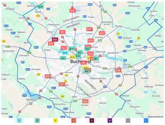
Figure 1.
Map showing the location of stations, from www.calitateaer.ro, accessed on 20 January 2025 (1—Good, 2—Acceptable, 3—Moderate, 4—Bad, 5—Very bad, 6—Extremely bad, Grey—Missing data, Blue—Insufficient data).
The concentration values for PM10 µg/m3, PM2.5µg/m3, and NO2 µg/m3 in Bucharest for last five years are presented in Table 1.

Table 1.
The mean values concentration for PM10, PM2.5, and NO2 µg/m3 in the last five years.
Constant high values for PM10 µg/m3 and PM2.5 µg/m3 were recorded at station B-1, while high values for NO2 were recorded at station B-6 (Table 1). The values from station B-1 were used for PM10 and PM2.5, and the values from station B-6 were used for NO2 within this paper. Also, we chose the Teom analyzer, due to it being more precise.
Constant high values for NO2 µg/m3 were recorded at station B-6 (Table 1), which was used within this paper. The mean value from 2023 remains critical.
4.2. Exploratory Data Analysis
Statistical calculations were applied to datasets on that period using method describe() in Python (Table 2).
Table 2.
Descriptive statistics for each pollutant.
Appendix A provides detailed visualizations supporting the main findings. Figure A1, Figure A2, Figure A3, Figure A4, Figure A5, Figure A6, Figure A7, Figure A8, Figure A9, Figure A10, Figure A11 and Figure A12 depicts the temporal evolution of training, reference, and testing datasets for PM10, PM2.5, and NO2. These plots showcase the consistency of the datasets and the alignment of predicted pollutant concentrations with observed values across different forecasting horizons, emphasizing the hybrid model’s accuracy in capturing both seasonal trends and deviations.
The non-stationarity suggested by the value of standard deviation in the time series was analyzed by plotting the time series, which can also help show trends and seasonality (Figure 2).
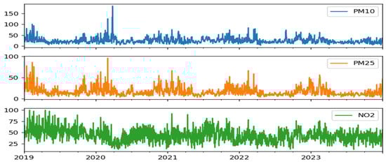
Figure 2.
Dataset time series.
We confirmed that our time series is non-stationary by using two tests: the Augmented Dickey–Fuller (ADF) test and the Kwiatkowski–Phillips–Schmidt–Shin (KPSS) test. The values for each test are presented in Table 3.
Table 3.
ADF and KPSS tests.
Overall, while the ADF test strongly suggests stationarity for all pollutants, the KPSS test’s borderline p-value indicates the potential for non-stationarity, hinting that the series may require further consideration or transformation.
We used the decompose method to determine what may need to be removed from the time series to fix it. We applied the decompose method for the entire period (Figure 3a–c).
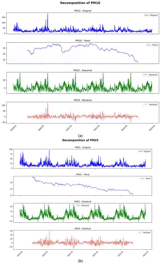
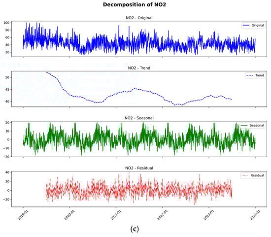
Figure 3.
(a) Decompose method for PM10. (b) Decompose method for PM2.5. (c) Decompose method for NO2.
ARIMA models handle seasonality and non-stationarity well, but they do not handle changes in variance or heteroskedasticity especially well. When one encounters heteroskedasticity in a time series, it is common to use a log transformation to manage it. One tool for performing this is the Box-Cox transformation. We applied a Box-Cox transformation to the data with the Box-Cox method and noted the results (Figure 4a–c).
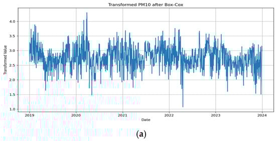
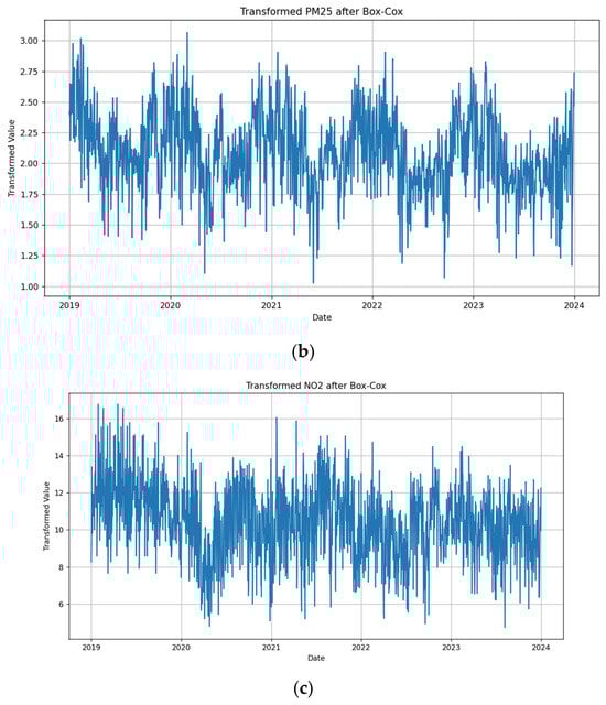
Figure 4.
(a) Transformed PM10 after Box-Cox. (b) Transformed PM2.5 after Box-Cox. (c) Transformed NO2 after Box-Cox.
The Box-Cox transformation applied λ values of −0.077, −0.188, and 0.477 for PM10, PM2.5, and NO2, respectively, determined using maximum log-likelihood estimation to minimize heteroskedasticity and stabilize variance.
The autocorrelations were plotted to notice the correlation between the points up to and including the lag unit. The autocorrelation function (ACF) and the partial autocorrelation function (PACF) are depicted in Figure 5a–c.
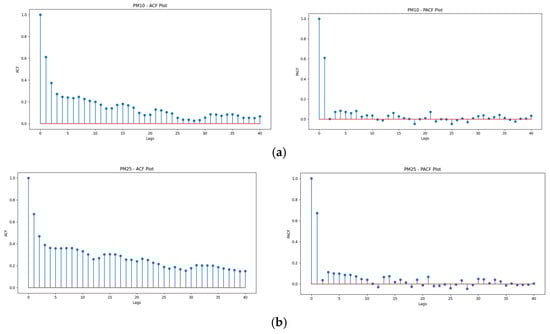
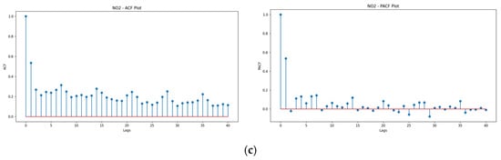
Figure 5.
(a) ACF and PACF result plotted for PM10. (b) ACF and PACF result plotted for PM2.5. (c) ACF and PACF result plotted for NO2.
The ACF and PACF plots for PM10, PM2.5, and NO2 reveal distinct temporal dependencies, providing insights into their autoregressive behavior and stationarity. For PM10, the ACF exhibits a sharp decline after lag 1, while the PACF shows a significant spike at lag 1 with minor contributions at subsequent lags, indicating strong short-term autocorrelation and suggesting an AR(1) or AR(2) process. In the case of PM2.5, the slow decay of the ACF combined with the PACF’s sharp cutoff at lag 1 or 2 suggests the presence of long-term autocorrelation, characteristic of non-stationary behavior that may require differencing, making an ARIMA(1,1,0) or ARIMA(2,1,0) model a likely candidate. For NO2, the gradual decline in the ACF and persistent PACF spikes at lag 1 and beyond point toward extended temporal dependencies, highlighting the need for autoregressive terms to capture higher-order relationships. Overall, the plots confirm the presence of short and long-term patterns, indicating that appropriate ARIMA models with autoregressive components and potential differencing are necessary for robust time series forecasting.
4.3. ARIMA and SARIMA
We performed a grid search around the values previously derived from ACF, PACF, and p value. The results, including RMSE calculation for all pollutants, are presented in Table 4.
Table 4.
Comparison of ARIMA models using RMSE and MAE values for PM10, PM2.5, and NO2.
The error metrics lead to applying SARIMA. The best SARIMA model for PM10 is SARIMAX(4, 0, 2)x(0, 0, [1], 12), where the seasonal components of the SARIMAX model are as follows: when the seasonal autoregressive = 0, it means there is no seasonal AR component; when the seasonal differencing = 0, it means no differencing is applied to account for seasonality; when the seasonal moving average order = 1, it means there is a first-order seasonal MA component; the period of seasonality = 12. Here, the time series has a yearly seasonality presumed to be monthly data, with 12 months in a year. The values for AIC and RMSE for all pollutants are presented in Table 5.
Table 5.
SARIMA model with AIC and RMSE values for PM10, PM2.5, NO2.
The AIC of the SARIMA model generated for all the pollutants is less than the non-seasonal model we created previously (Table 5). This could indicate that the seasonal component is an important feature for our modeling. Also, the RMSE values for our Seasonal ARIMA model are much smaller than for the non-Seasonal ARIMA model for all pollutants.
Next, we used the residuals as inputs for BiLSTM models. The residuals were obtained after applying SARIMAX with the seasonal order values derived from SARIMA analysis.
The evaluation of standalone SARIMA and hybrid SARIMA-BiLSTM models across all pollutants revealed distinct advantages in adopting hybrid approaches for air pollutant forecasting. Key performance metrics, including Root Mean Square Error (RMSE), Mean Absolute Error (MAE), and Mean Absolute Percentage Error (MAPE), were used to quantify the predictive accuracy and robustness of each model configuration. The results are detailed in Table 6.
Table 6.
Comparison of Best Parameters for Hybrid Time Series Models.
These configurations demonstrate the effectiveness of hybrid models in leveraging seasonal adjustments (via Fourier terms) and advanced architectures like LSTM, GRU, and Attention mechanisms to improve pollutant forecasting accuracy and address nonlinear dependencies.
4.4. Overall Performance of Models
The evaluation of standalone SARIMA and hybrid SARIMA-BiLSTM models across all pollutants revealed distinct advantages in adopting hybrid approaches for air pollutant forecasting. Key performance metrics, including Root Mean Square Error (RMSE), Mean Absolute Error (MAE), and Mean Absolute Percentage Error (MAPE), were used to quantify the predictive accuracy and robustness of each model configuration. The results are detailed in Table 7.
Table 7.
Performance metrics of SARIMA and hybrid models for pollutant forecasting.
4.5. Performance Metrics Comparison
Standalone SARIMA models served as the baseline for comparisons, delivering moderate performance across all pollutants. For example, SARIMA achieved RMSE values of 0.164 for PM10, 0.106 for PM2.5, and 0.700 for NO2 over a 1-day forecasting horizon (Table 7). While these results demonstrate SARIMA’s ability to model linear dependencies and seasonal patterns, the residuals showed significant autocorrelation and variance (refer to Table 8), limiting its accuracy, particularly for pollutants with nonlinear dynamics.
Table 8.
Comparison of Forecasting Models for PM10, PM2.5, and NO2: RMSE, MAE, and MAPE Across Different Horizons.
Hybrid models consistently outperformed standalone SARIMA, particularly in capturing nonlinear and seasonal dependencies. The SARIMA + BiLSTM configuration demonstrated notable improvements, with RMSE reductions of 3.0–11.0% across pollutants compared to standalone SARIMA (Table 7). For PM10, the hybrid model reduced RMSE from 0.164 to 0.159 and MAPE from 6.79% to 6.55%. Similarly, for PM2.5, the SARIMA + BiLSTM model achieved an RMSE of 0.094, significantly improving on SARIMA’s RMSE of 0.106. For NO2, where variability is higher, SARIMA + BiLSTM + Attention provided marginal reductions in RMSE (0.694) compared to SARIMA (0.700), highlighting the importance of advanced mechanisms in managing extreme deviations and variability.
4.6. Horizon-Specific Analysis of Forecasting Models
The forecasting models were further evaluated across three time horizons: 1-day, 7-days, and 30-days (Table 8). For PM10, SARIMA + BiLSTM(GRU) exhibited superior performance across all horizons, particularly for the 30-day forecast, achieving an RMSE of 0.1692, MAE of 0.1285, and MAPE of 6.03%. The SARIMA + BiLSTM + Attention model performed best for short-term forecasts, with the lowest RMSE (0.1379) for the 1-day horizon. Notably, SARIMA + Fourier + BiLSTM displayed lower performance variability across horizons, indicating its robustness for medium-range predictions.
For PM2.5 (Table 8), SARIMA + BiLSTM(GRU) again demonstrated high accuracy for the 1-day horizon (RMSE: 0.0715) and comparable performance over longer horizons. SARIMA + BiLSTM + Attention provided the most consistent improvements in MAPE across horizons, with the lowest MAPE for the 30-day horizon (4.32%). This suggests its suitability for maintaining percentage accuracy in long-term forecasts.
For NO2 (Table 8), performance across horizons varied significantly. SARIMA + BiLSTM and SARIMA + BiLSTM(GRU) achieved comparable results for the 1-day and 7-day horizons, with RMSE values of 0.7104 and 0.7254, respectively. However, for the 30-day horizon, SARIMA + Fourier + BiLSTM showed a notable RMSE improvement (0.6766) compared to other models, indicating its potential for capturing long-term patterns.
4.7. Horizon-Specific Analysis of Forecasting Performance
The performance of the forecasting models was assessed across three horizons: 1-day, 7-days, and 30-days. Each horizon posed distinct challenges, with accuracy decreasing as the forecasting period extended due to compounding uncertainties and increasing complexity.
For the 1-day horizon, models demonstrated the highest accuracy due to the limited temporal gap and reliance on recent data. SARIMA + BiLSTM(GRU) and SARIMA + BiLSTM achieved identical performance metrics for PM10, with an RMSE of 0.1376 and a MAPE of 5.52%. The addition of attention mechanisms, as in SARIMA + BiLSTM + Attention, resulted in comparable RMSE values (0.1379) but a marginally higher MAPE (5.53%). For PM2.5, SARIMA + BiLSTM(GRU) and SARIMA + BiLSTM provided the best results with an RMSE of 0.0715 and a MAPE of 3.92%, slightly outperforming SARIMA + BiLSTM + Attention, which recorded an RMSE of 0.0732 and a MAPE of 3.97%. In contrast, SARIMA + Fourier + BiLSTM displayed relatively lower performance for both pollutants, indicating limited utility of Fourier-transform enhancements for short-term predictions. The NO2 forecasts revealed that SARIMA + BiLSTM(GRU) and SARIMA + BiLSTM performed similarly, with an RMSE of 0.7104 and a MAPE of 7.93%, while SARIMA + Fourier + BiLSTM exhibited the highest RMSE (0.7203) and MAPE (8.04%) among the models tested.
As the forecasting horizon extended to 7 days, performance declined moderately as models encountered nonlinear dynamics and cumulative errors. For PM10, SARIMA + BiLSTM + Attention slightly outperformed other models, achieving an RMSE of 0.1416 and a MAPE of 5.66%, while SARIMA + BiLSTM and SARIMA + BiLSTM(GRU) maintained similar performance levels, with RMSE values of 0.1428 and a MAPE of 5.73%. SARIMA + Fourier + BiLSTM showed reduced accuracy for this horizon, with an RMSE of 0.1450 and a MAPE of 5.86%. The PM2.5 forecasts indicated near-identical results for SARIMA + BiLSTM(GRU) and SARIMA + BiLSTM, both achieving an RMSE of 0.0737 and a MAPE of 4.05%, whereas SARIMA + BiLSTM + Attention demonstrated a slightly higher RMSE of 0.0745 but comparable MAPE (4.04%). For NO2, SARIMA + BiLSTM + Attention marginally improved upon the other hybrid models, recording a lower MAPE (7.84%) despite a higher RMSE (0.7273), whereas SARIMA + Fourier + BiLSTM continued to underperform, particularly in terms of RMSE (0.7366) and MAPE (8.02%).
The 30-day horizon posed significant challenges due to the accumulation of uncertainty over time. For PM10, SARIMA + BiLSTM(GRU) provided the most accurate predictions, with an RMSE of 0.1692, MAE of 0.1285, and a MAPE of 6.03%. SARIMA + BiLSTM + Attention demonstrated strong performance with an RMSE of 0.1473 and a MAPE of 5.93%, suggesting its robustness for capturing extended temporal dependencies. Interestingly, SARIMA + Fourier + BiLSTM exhibited improved performance relative to intermediate horizons, achieving an RMSE of 0.1574 and a MAPE of 5.45%. In the case of PM2.5, SARIMA + BiLSTM and SARIMA + BiLSTM(GRU) delivered satisfactory results with RMSE values of 0.0822 and 0.0992, respectively, while SARIMA + BiLSTM + Attention demonstrated the lowest MAPE (4.32%) across all models, making it particularly suited for long-term relative accuracy. NO2 forecasts revealed that SARIMA + Fourier + BiLSTM outperformed other models for the 30-day horizon, achieving an RMSE of 0.6766 and a MAPE of 7.37%. Although SARIMA + BiLSTM and SARIMA + BiLSTM(GRU) had slightly higher RMSE values (0.6652), they demonstrated lower MAPE (7.22%), indicating a strong ability to maintain percentage-based accuracy for extended forecasts.
This analysis highlights the relationship between forecasting accuracy and horizon length, with short-term predictions benefiting from simpler temporal dynamics and long-term forecasts posing greater challenges. Hybrid models integrating BiLSTM architecture consistently provided enhanced accuracy across horizons, particularly for pollutants with nonlinear temporal behaviors. The inclusion of attention mechanisms further refined performance in intermediate and long-term predictions, particularly for MAPE, while Fourier-enhanced models demonstrated robustness for pollutants with smoother patterns, such as NO2. These findings underscore the need to select models tailored to specific pollutants and forecasting horizons for optimal performance.
4.8. Pollutant-Specific Analysis
4.8.1. PM10
The forecasting performance for PM10 demonstrated the strengths and limitations of different model configurations. The SARIMA + BiLSTM(GRU) hybrid model consistently achieved the best performance across both short-term and long-term horizons. For the 1-day horizon, this model recorded an RMSE of 0.1376 and a MAPE of 5.52%, maintaining accuracy even over extended forecasts, such as the 30-day horizon, where it achieved an RMSE of 0.1692 and a MAPE of 6.03% (Table 8). These results highlight its capability to effectively capture the complex temporal dynamics of PM10 concentrations, which include both seasonal and nonlinear patterns.
In contrast, Fourier-enhanced models, such as SARIMA + Fourier and SARIMA + BiLSTM + Fourier, showed limitations in handling the nonlinear dependencies inherent in PM10 data. While the inclusion of Fourier terms improved the modeling of seasonal trends, these models struggled with the pollutant’s abrupt variations and nonlinear patterns. For example, the SARIMA + Fourier model recorded an RMSE of 0.166 and a MAPE of 6.91%, which were higher than those of BiLSTM-based hybrids (Table 7). This underscores the importance of integrating advanced machine learning components, such as BiLSTM, to address PM10’s unique characteristics.
4.8.2. PM2.5
For PM2.5, the SARIMA + BiLSTM(GRU) model demonstrated superior performance, achieving the lowest RMSE and MAPE among all configurations. With an RMSE of 0.093 and a MAPE of 5.33%, it significantly outperformed the standalone SARIMA model, which recorded an RMSE of 0.106 and a MAPE of 5.86% (Table 7). The SARIMA + BiLSTM(GRU) model’s ability to effectively handle both linear and nonlinear dependencies in PM2.5 data positions it as the most reliable choice for this pollutant.
The integration of attention mechanisms further refined forecast precision, particularly for longer horizons. The SARIMA + BiLSTM + Attention model achieved the lowest MAPE of 4.32% for the 30-day horizon, emphasizing its effectiveness in scenarios requiring high percentage accuracy (Table 8). By prioritizing influential temporal features, attention mechanisms enhanced the interpretability and precision of predictions, making them particularly valuable for PM2.5, where maintaining relative accuracy is important.
4.8.3. NO2
NO2 presented significant challenges for forecasting due to its higher variability and frequent extreme values. The standalone SARIMA model provided a competitive baseline, achieving an RMSE of 0.700 and a MAPE of 7.62% for the 1-day horizon (Table 8). However, the pollutant’s complex dynamics and deviations necessitated advanced modeling techniques.
Hybrid models incorporating BiLSTM and attention mechanisms offered marginal improvements. The SARIMA + BiLSTM + Attention model recorded a slightly reduced RMSE of 0.694 and a MAPE of 7.71% compared to SARIMA alone (Table 7). Despite these enhancements, the high variability of NO2 limited the extent of improvement achievable with existing hybrid configurations. The Fourier-enhanced models also faced challenges, with SARIMA + Fourier + BiLSTM achieving an RMSE of 0.6766 for the 30-day horizon, demonstrating potential in capturing smoother seasonal patterns but falling short in handling extreme deviations.
Overall, NO2’s forecasting results emphasize the need for additional innovations, such as ensemble modeling or specialized loss functions, to address its unique characteristics. While hybrid models demonstrated incremental progress, further refinement is necessary to enhance robustness in managing extreme variability and abrupt shifts in NO2 concentrations.
4.9. Analysis of Residual Variance and Metrics
Residual variance analysis provides important insights into model performance by examining the statistical properties of residuals, including their mean, standard deviation, skewness, kurtosis, and independence (Table 9). These metrics help assess whether the residuals adhere to assumptions of normality, homoscedasticity, and independence, which are important for reliable model performance.
Table 9.
Residual statistical analysis and model diagnostics for pollutant forecasting.
4.9.1. PM10 Residuals
For PM10, the standalone SARIMA model exhibited a residual mean of 0.0324 and a standard deviation of 0.1607, with negative skewness (−0.4345) and kurtosis (−0.5624). These values suggest asymmetry and a deviation from normality. The Durbin–Watson statistic (0.9349) indicates potential autocorrelation, supported by the low Ljung–Box p-value (7.45 × 10⁻⁸), signaling dependence in residuals.
Hybrid models incorporating BiLSTM architectures significantly improved the residual statistics. SARIMA + BiLSTM reduced the mean to 0.0047 and achieved a slightly lower standard deviation (0.1591). Similarly, SARIMA + BiLSTM(GRU) further improved these metrics with a mean of 0.0158 and standard deviation of 0.1580. Both models increased the Durbin–Watson statistic (1.0233 and 1.0523, respectively), reducing autocorrelation compared to SARIMA. The Ljung–Box p-value, while still small, was higher than that of SARIMA, indicating improved residual independence.
Models augmented with Fourier components showed mixed performance. SARIMA + Fourier maintained a high mean (0.0316) and standard deviation (0.1630), with metrics closely resembling SARIMA, suggesting limited improvement. However, SARIMA + BiLSTM + Fourier achieved the lowest residual mean (0.00176), indicating enhanced accuracy, though the Ljung–Box p-value (3.95 × 10⁻⁷) and Durbin–Watson statistic (0.9617) reflect persistent challenges with independence.
The SARIMA + BiLSTM + Attention model balanced residual properties well, achieving a mean of 0.0056 and a standard deviation of 0.1629. While skewness and kurtosis improved slightly, the model’s Ljung–Box p-value remained low (3.93 × 10⁻⁸), highlighting persistent autocorrelation challenges.
4.9.2. PM2.5 Residuals
For PM2.5, SARIMA residuals exhibited a mean of 0.0544, a standard deviation of 0.0867, and moderate departures from normality (skewness: −0.2375, kurtosis: −0.3412). The Durbin–Watson statistic (0.7224) and Ljung–Box p-value (4.37 × 10⁻⁷) suggested significant autocorrelation and residual dependence.
The hybrid models reduced residual variance effectively. SARIMA + BiLSTM lowered the mean to 0.0392 and standard deviation to 0.0857, with improved Durbin–Watson statistics (0.8664). SARIMA + BiLSTM(GRU) performed similarly, achieving a residual mean of 0.0367 and a standard deviation of 0.0856. Both models demonstrated reduced autocorrelation, though their Ljung–Box p-values (1.06 × 10⁻⁶ and 9.89 × 10⁻⁷, respectively) remained low, indicating lingering dependence.
Fourier-enhanced models yielded higher residual means and standard deviations compared to BiLSTM-based models. SARIMA + Fourier had a mean of 0.0586 and a standard deviation of 0.0878, showing limited improvement over SARIMA. However, SARIMA + BiLSTM + Fourier and SARIMA + BiLSTM + Attention exhibited better residual characteristics, with SARIMA + BiLSTM + Attention achieving a residual mean of 0.0432 and a Durbin–Watson statistic of 0.8266, reducing autocorrelation to some extent.
4.9.3. NO2 Residuals
For NO2, SARIMA residuals showed higher variability, with a mean of 0.1102 and a standard deviation of 0.6912. Skewness (−0.2621) and kurtosis (−0.5190) indicated deviations from normality. The Durbin–Watson statistic (1.3279) suggested lower autocorrelation compared to PM10 and PM2.5, but the Ljung–Box p-value (2.22 × 10⁻⁴) highlighted residual dependence.
Hybrid models improved residual properties moderately. SARIMA + BiLSTM reduced the mean to 0.0691, though the standard deviation increased slightly (0.7041). SARIMA + BiLSTM(GRU) and SARIMA + BiLSTM + Fourier exhibited comparable residual means (0.0771 and 0.0225, respectively) and standard deviations (0.7068 and 0.7100), with marginal improvements in Durbin–Watson statistics (1.3205 and 1.3524, respectively).
The SARIMA + BiLSTM + Attention model achieved the best results, with a residual mean of −0.0148 and a standard deviation of 0.6943. The Durbin–Watson statistic (1.3565) and Ljung–Box p-value (2.07 × 10⁻⁴) highlighted its ability to reduce autocorrelation compared to other hybrid models.
Residual analysis underscores the advantages of hybrid SARIMA models for reducing mean residual error and standard deviation, particularly in PM10 and PM2.5 predictions. However, the persistence of low Ljung–Box p-values across all pollutants and models highlights residual dependence challenges, suggesting that further refinements in hybrid modeling strategies are needed to improve independence. SARIMA + BiLSTM and SARIMA + BiLSTM + Attention consistently outperformed Fourier-augmented models, demonstrating the efficacy of deep learning components in capturing nonlinear temporal dependencies. These findings emphasize the importance of combining statistical preprocessing with advanced machine learning techniques to enhance pollutant prediction accuracy.
4.10. Extreme Values Analysis Across Models
Extreme value analysis (Table 10) examines the performance of forecasting models under conditions where deviations from typical pollutant levels occur. Metrics such as RMSE, MAE, and MAPE provide insights into the models’ ability to handle outliers, abrupt changes, or high variability in pollutant data. This analysis is important for evaluating model robustness and reliability in scenarios that significantly impact decision-making and environmental monitoring.
Table 10.
Performance metrics for extreme value handling across models and pollutants.
4.10.1. PM10 Extreme Value Performance
For PM10, SARIMA achieved relatively low RMSE (0.310), MAE (0.306), and MAPE (18.16%), indicating moderate performance in capturing extreme values. However, hybrid models introduced variability in performance. SARIMA + BiLSTM exhibited increased RMSE (0.339) and MAPE (19.68%), suggesting challenges in managing large deviations effectively. Similarly, SARIMA + BiLSTM(GRU) slightly improved over SARIMA + BiLSTM with a lower RMSE (0.329) and MAPE (18.97%) but still lagged behind the baseline SARIMA model.
Fourier-enhanced models demonstrated a mixed response. SARIMA + Fourier recorded an RMSE of 0.312, marginally higher than SARIMA, with a comparable MAPE of 18.31%. The integration of Fourier components with BiLSTM architectures resulted in increased errors; SARIMA + BiLSTM + Fourier had the highest RMSE (0.339) and MAPE (19.85%) among all models, reflecting potential overfitting or inefficiencies in capturing extreme events. SARIMA + BiLSTM + Attention slightly reduced these errors, achieving an RMSE of 0.335 and MAPE of 19.61%.
4.10.2. PM2.5 Extreme Value Performance
For PM2.5, all models demonstrated a smaller range of RMSE and MAPE compared to PM10, indicating greater stability in handling extreme values. The baseline SARIMA model recorded an RMSE of 0.174 and a MAPE of 11.67%, establishing a benchmark for comparison.
Hybrid models consistently outperformed SARIMA, with SARIMA + BiLSTM achieving a reduced RMSE of 0.167 and MAPE of 11.54%. SARIMA + BiLSTM(GRU) provided marginal improvements, with the lowest RMSE (0.166) and MAPE (11.51%) among all models, reflecting its ability to manage extreme deviations effectively. Fourier-based models showed moderate improvement. SARIMA + Fourier matched SARIMA in RMSE (0.174) but achieved a slightly reduced MAPE (11.59%). SARIMA + BiLSTM + Fourier and SARIMA + BiLSTM + Attention performed similarly, with RMSE values of 0.170 and 0.168, respectively, and both recorded a MAPE of 11.54%.
4.10.3. NO2 Extreme Value Performance
Extreme value analysis for NO2 revealed higher overall errors compared to PM10 and PM2.5, emphasizing the challenges posed by the pollutant’s greater variability and more pronounced deviations. SARIMA exhibited an RMSE of 1.581 and a MAPE of 25.07%, setting the baseline for comparison.
Hybrid models incorporating BiLSTM generally struggled with NO2 extremes. SARIMA + BiLSTM recorded higher RMSE (1.625) and MAPE (25.85%) than SARIMA, and SARIMA + BiLSTM(GRU) offered negligible improvement with an RMSE of 1.624 and MAPE of 25.84%. Fourier-based models showed similar performance trends, with SARIMA + Fourier achieving a marginally higher RMSE (1.585) than SARIMA and an identical MAPE (25.10%). However, the combination of Fourier and BiLSTM components in SARIMA + BiLSTM + Fourier resulted in the highest RMSE (1.659) and MAPE (26.38%) among all models, indicating limited effectiveness in handling extreme NO2 values. SARIMA + BiLSTM + Attention slightly improved on this with an RMSE of 1.643 and a MAPE of 26.15%.
5. Discussions and Implications
This study advances air quality forecasting by integrating SARIMA with Bidirectional Long Short-Term Memory (BiLSTM) networks, augmented by Box-Cox transformations, Fourier terms, and attention mechanisms. The findings highlight methodological and practical innovations that address challenges in pollutant forecasting, including nonlinear dependencies, seasonality, and extreme values.
While the hybrid models demonstrated notable improvements for PM10 and PM2.5, their performance for NO2 forecasts indicates areas for further refinement. The results suggest that hybrid approaches, while promising, are pollutant-specific and should not be generalized as universally applicable solutions for air quality. The term “air quality improvement” is used strictly in the context of forecasting accuracy rather than mitigation strategies.
5.1. Comparison with Existing Literature
The incorporation of hybrid models aligns with existing research, emphasizing their ability to leverage the strengths of statistical methods like SARIMA for linear trends and machine learning models for nonlinear dependencies. For example, Alhirmizy and Qader (2019) [19] demonstrated the efficacy of LSTM networks for multivariate time-series air quality forecasting in Madrid, Spain, achieving high accuracy for pollutants such as NO2 and CO. Similarly, Ansari and Alam (2024) [15] combined SARIMA and LSTM, fine-tuned using Bayesian optimization, achieving superior performance compared to standalone models.
This study builds on these advancements by incorporating Fourier terms for enhanced seasonal modeling and attention mechanisms for prioritizing influential temporal features. Compared to standalone SARIMA or BiLSTM models, the SARIMA + BiLSTM + Fourier hybrid approach demonstrates consistent improvements in RMSE and MAPE values, particularly for PM2.5 and PM10. For instance, the RMSE for PM2.5 predictions decreased from 0.100 in SARIMA + Fourier to 0.094 in SARIMA + BiLSTM + Fourier, underscoring the complementary nature of these components. These results echo the findings of Aram et al. (2024) [26], who reported significant gains in air quality forecasting by integrating machine learning and statistical methods.
5.2. Impact of Box-Cox Transformation and Fourier Terms
The inclusion of the Box-Cox transformation and Fourier terms was important in stabilizing variance and enhancing the modeling of seasonal patterns. As shown in Figure 4a–c, the Box-Cox transformation effectively reduced heteroskedasticity, preparing the time series data for improved forecasting accuracy. Fourier terms modeled annual seasonality efficiently, as evidenced by the performance of SARIMA + Fourier models, which demonstrated moderate improvements over standalone SARIMA. For instance, SARIMA + Fourier achieved an RMSE of 0.166 for PM10 and 0.100 for PM2.5, slightly outperforming SARIMA but lagging behind hybrid models that integrated BiLSTM components.
The hybrid models’ ability to incorporate both stabilized variance from Box-Cox and seasonal trends from Fourier terms further enhanced their predictive power. SARIMA + BiLSTM + Fourier models achieved balanced performance across pollutants, offering improved RMSE and MAPE values compared to SARIMA + Fourier alone. For instance, for PM2.5, the RMSE dropped from 0.100 in SARIMA + Fourier to 0.094 in SARIMA + BiLSTM + Fourier (Table 7).
Integrating these preprocessing techniques into hybrid models yielded further gains. For example, SARIMA + BiLSTM + Fourier outperformed SARIMA + Fourier alone in both short- and long-term horizons, highlighting the importance of combining statistical preprocessing with deep learning techniques.
These findings support the observations of Borhani et al. (2023) [11], who emphasized the role of robust statistical transformations in improving air pollutant trend predictions. By addressing both linear and nonlinear dependencies, the proposed hybrid framework demonstrates broader applicability and enhanced predictive power.
5.3. Extreme Value Analysis
The analysis highlights notable differences in the models’ ability to handle extreme pollutant values. For PM10, standalone SARIMA showed competitive performance, while hybrid models incorporating BiLSTM exhibited increased error rates, potentially due to sensitivity to abrupt changes. In contrast, PM2.5 predictions showed greater consistency, with SARIMA + BiLSTM(GRU) emerging as the most robust model for managing extreme deviations. For NO2, the high variability and presence of extreme values proved challenging across all models, with Fourier-enhanced models and BiLSTM hybrids demonstrating increased error rates.
These findings underscore the importance of tailoring hybrid model architectures to specific pollutant characteristics. While deep learning components like BiLSTM can enhance overall accuracy, their effectiveness in handling extreme values requires further refinement. Incorporating domain-specific preprocessing, such as robust outlier handling and feature engineering, may enhance the models’ resilience to extreme conditions, ensuring more reliable forecasting for decision-making scenarios.
Forecasting extreme pollutant values remains a challenge due to their rarity and disproportionate impact. The SARIMA + BiLSTM hybrid model showed improved performance in capturing these anomalies compared to traditional SARIMA models. However, variability in pollutant behavior, particularly for NO2, posed difficulties, with Fourier-enhanced models exhibiting increased error rates for extreme values.
This aligns with findings by Nath et al. (2023) [25], who reported that transformer-based neural network architectures struggled with extreme value modeling compared to hybrid statistical and machine learning methods. For PM2.5, the SARIMA + BiLSTM(GRU) configuration proved particularly effective, achieving consistent performance across short- and long-term horizons. These results suggest that while hybrid models offer significant improvements, further refinement is needed to enhance their resilience to extreme conditions.
5.4. Practical Implications for Air Quality Forecasting
The results underscore the potential of hybrid models for real-world air quality forecasting and decision-making. The SARIMA + BiLSTM + Attention model demonstrated robust performance for percentage-sensitive metrics like MAPE, making it suitable for applications requiring precise error minimization. The comparative stability of these models across horizons highlights their utility for dynamic air quality monitoring in urban settings.
Integrating these models into IoT-based frameworks, as proposed by Bhatia et al. (2023) [29], could enable real-time updates and location-specific forecasts. This study’s findings also resonate with the work of Das et al. (2021) [22], who highlighted the need for hybrid approaches to address the complex temporal and spatial patterns of air pollution.
5.5. Cross-Horizon Observations
A key observation across pollutants is the relative stability of hybrid models incorporating BiLSTM architectures. The addition of GRU and attention mechanisms provided marginal gains for short-term horizons but did not consistently translate into better long-term performance. Furthermore, Fourier-transform-enhanced models exhibited variability, performing better in scenarios with smoother temporal variations.
The SARIMA + BiLSTM + Attention model consistently maintained low MAPE values, underscoring its effectiveness in percentage-error-sensitive applications. However, the marginally higher RMSE in several cases suggests a trade-off between absolute error minimization and interpretability offered by attention mechanisms.
The hybrid modeling approach, combining SARIMA residuals with BiLSTM architectures, effectively captured both linear and nonlinear dependencies in pollutant data. By using SARIMA residuals preprocessed with the Box-Cox transformation, the models leveraged stabilized variance and reduced noise. This preprocessing step was particularly beneficial for BiLSTM networks, enabling them to learn intricate temporal patterns without the need for additional inverse transformations. These results highlight the importance of integrating statistical preprocessing with deep learning techniques for robust pollutant forecasting.
The horizon-specific evaluation revealed the challenges of maintaining accuracy over longer horizons, particularly for NO2, where variability in pollutant levels proved challenging to model. Future research could explore ensemble techniques and model fine-tuning for improved stability and performance across diverse time scales. The horizon-specific analysis revealed that while short-term forecasts benefitted significantly from attention mechanisms, long-term predictions exhibited higher variability. The SARIMA + BiLSTM + GRU configuration emerged as the most robust for extended horizons, achieving an RMSE improvement of up to 11% compared to Fourier-augmented models for pollutants like PM10. These observations are consistent with Dutta and Pal (2023) [27], who demonstrated the advantages of deep transfer learning models for long-term air quality predictions.
5.6. Methodological Contributions
This study’s integration of statistical preprocessing, such as Box-Cox transformations, with advanced neural architectures addresses key limitations of traditional and machine learning models. The use of Fourier terms for seasonal decomposition, combined with BiLSTM’s bidirectional learning capabilities, enhances the model’s ability to capture both cyclical patterns and complex temporal dependencies. The results align with Freeman et al. (2018) [24], who emphasized the importance of preprocessing in improving the interpretability and accuracy of deep learning models for air quality forecasting.
5.7. Future Directions
While the proposed hybrid framework offers significant advancements, further research is needed to refine its applicability to diverse pollutants and geographic regions. Incorporating ensemble methods and exploring domain-specific preprocessing, such as robust outlier detection, could enhance the models’ resilience to extreme values. Additionally, expanding datasets to include real-time and spatiotemporal data, as demonstrated by Chen et al. (2024) [28], could improve scalability and generalizability.
In conclusion, this study highlights the potential of hybrid SARIMA + BiLSTM models for advancing air quality forecasting. By integrating robust statistical preprocessing with state-of-the-art deep learning techniques, it provides actionable insights for managing and mitigating air pollution in diverse environmental contexts.
6. Conclusions
Comparative analysis underscores the performance of hybrid models, particularly SARIMA + BiLSTM configurations, in achieving lower RMSE and MAPE values for pollutants such as PM10 and PM2.5. These configurations demonstrate notable advancements over traditional standalone approaches, especially in addressing nonlinear behaviors and extended temporal dependencies in pollutant data. The integration of attention mechanisms further enhances predictive accuracy, making these models effective in scenarios requiring precise error minimization, such as percentage-based accuracy assessments.
Despite significant improvements in short- and medium-term forecasting, challenges persist in managing long-term predictions and extreme pollutant values, particularly for NO2. These findings highlight the need for further methodological advancements, including the development of ensemble techniques and domain-specific preprocessing strategies, to bolster model robustness and adaptability in complex forecasting scenarios.
The proposed hybrid framework offers valuable insights for policymakers and urban planners, providing enhanced accuracy and interpretability in air quality predictions. Its scalability and adaptability position it as a promising solution for practical applications, such as smart city initiatives and IoT-based air quality monitoring systems. Future research should aim to extend the framework’s applicability to a broader range of pollutants and geographic contexts, leveraging real-time and spatiotemporal datasets to improve generalizability and scalability further.
Author Contributions
Conceptualization, I.H., L.H. and D.F.; methodology, S.-C.N.; software, I.H. and S.-C.N.; validation, L.H. and D.F.; formal analysis, S.-C.N.; investigation, I.H.; resources, L.H. and S.-C.N.; data curation, I.H.; writing—original draft preparation, L.H. and S.-C.N.; writing—D.F., L.H. and S.-C.N.; visualization, I.H. and S.-C.N. All authors have read and agreed to the published version of the manuscript.
Funding
This research received no external funding.
Data Availability Statement
Dataset available on request from the authors.
Conflicts of Interest
The authors declare no conflicts of interest.
Appendix A
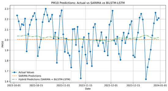
Figure A1.
PM10 Predictions: Actual vs. SARIMA vs. Hybrid (SARIMA + LSTM).
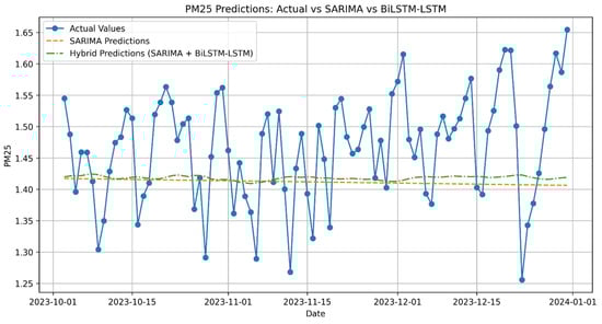
Figure A2.
PM2.5 Predictions: Actual vs. SARIMA vs. Hybrid (SARIMA + LSTM).
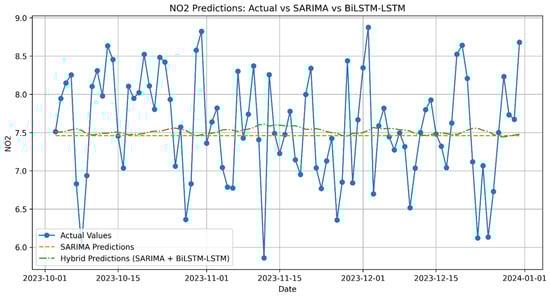
Figure A3.
NO2 Predictions: Actual vs. SARIMA vs. Hybrid (SARIMA + LSTM).
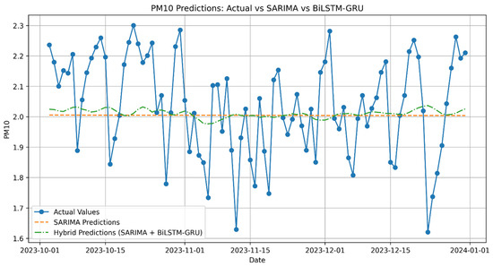
Figure A4.
PM10 Predictions: Actual vs. SARIMA vs. Hybrid (SARIMA + BiLSTM-GRU).
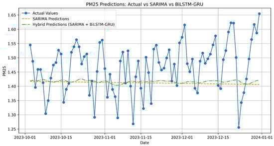
Figure A5.
PM2.5 Predictions: Actual vs. SARIMA vs. Hybrid (SARIMA + BiLSTM-GRU).
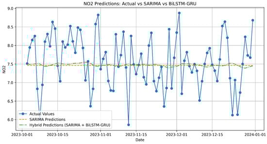
Figure A6.
NO2 Predictions: Actual vs. SARIMA vs. Hybrid (SARIMA + BiLSTM-GRU).
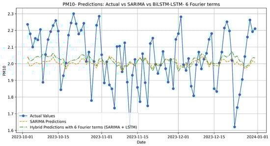
Figure A7.
PM10 Predictions: Actual vs. SARIMA vs. Hybrid with 6 Fourier terms (SARIMA + LSTM).
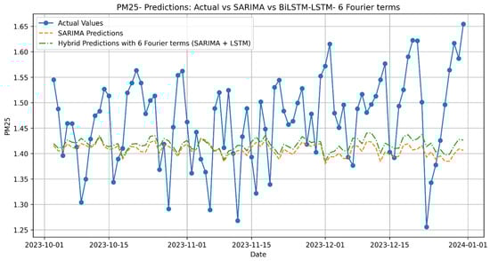
Figure A8.
PM2.5 Predictions: Actual vs. SARIMA vs. Hybrid with 6 Fourier terms (SARIMA + LSTM).
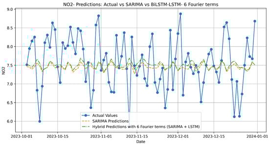
Figure A9.
NO2 Predictions: Actual vs. SARIMA vs. Hybrid with 6 Fourier terms (SARIMA + LSTM).
Figure A10.
PM10 Predictions: Actual vs. SARIMA vs. Hybrid (SARIMA + LSTM-Attention).
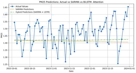
Figure A11.
PM2.5 Predictions: Actual vs. SARIMA vs. Hybrid (SARIMA + LSTM-Attention).
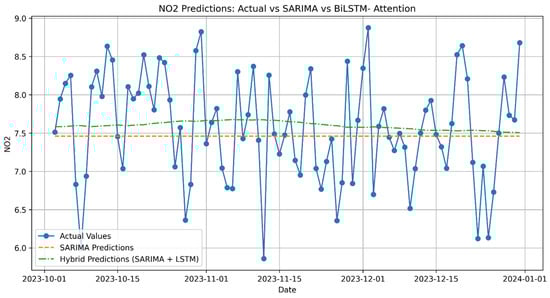
Figure A12.
NO2 Predictions: Actual vs. SARIMA vs. Hybrid (SARIMA + LSTM-Attention).
References
- European Environment Agency. Briefing no. 06/2024: Europe’s Air Quality Status. Available online: https://www.eea.europa.eu/publications/europes-air-quality-status-2024 (accessed on 17 November 2024).
- Southerland, V.; Brauer, M.; Mohegh, A.; Hammer, M.S.; van Donkelaar, A.; Martin, R.V.; Apte, J.S.; Anenberg, S.C. Global urban temporal trends in fine particulate matter (PM2·5) and attributable health burdens: Estimates from global datasets. Lancet Planet. Health 2022, 6, e139–e146. [Google Scholar] [CrossRef] [PubMed]
- WHO. New WHO Global Air Quality Guidelines Aim to Save Millions of Lives from Air Pollution 2021. Available online: https://www.who.int/news/item/22-09-2021-new-who-global-air-quality-guidelines-aim-to-save-millions-of-lives-from-air-pollution (accessed on 20 November 2024).
- European Environment Agency. European City Air Quality Viewer. Published at 21 August 2024. Available online: https://www.eea.europa.eu/en/topics/in-depth/air-pollution/european-city-air-quality-viewer (accessed on 5 December 2024).
- Airly. Air Pollution in Bucharest. What Are the Main Sources? Available online: https://airly.org/en/what-are-the-main-sources-of-air-pollution-in-bucharest/ (accessed on 6 December 2024).
- Li, Y.; Guo, J.; Sun, S.; Li, J.; Wang, S.; Zhang, C. Air quality forecasting with artificial intelligence techniques: A scientometric and content analysis. Environ. Model. Softw. 2022, 149, 105329. [Google Scholar] [CrossRef]
- Cabaneros, S.M.; Calautit, J.K.; Hughes, B.R. A review of artificial neural network models for ambient air pollution prediction. Environ. Model. Softw. 2019, 119, 285–304. [Google Scholar] [CrossRef]
- Jiang, P.; Dong, Q.; Li, P. A novel hybrid strategy for PM2.5 concentration analysis and prediction. J. Environ. Manag. 2017, 196, 443–457. [Google Scholar] [CrossRef] [PubMed]
- Hochreiter, S.; Schmidhuber, J. Long Short-term Memory. Neural Comput. 1997, 9, 1735–1780. [Google Scholar] [CrossRef]
- Ilie, A.; Vasilescu, J.; Talianu, C.; Iojă, C.; Nemuc, A. Spatiotemporal Variability of Urban Air Pollution in Bucharest City. Atmosphere 2023, 14, 1759. [Google Scholar] [CrossRef]
- Borhani, F.; Shafiepour Motlagh, M.; Rashidi, Y.; Ehsani, A.H. Estimation of short-lived climate forced sulfur dioxide in Tehran, Iran, using machine learning analysis. Stoch. Environ. Res. Risk Assess. 2022, 36, 2847–2860. [Google Scholar] [CrossRef]
- Sakib, S.R.; Sara, K.N.; Rasel, M.T.H.; Asif, M.M.I.; Nahid, M.A.H.; Rahman, M.S.; Islam, A. Time Series Analysis and Forecasting of Air Quality Index of Dhaka City of Bangladesh. In Proceedings of the 2023 IEEE World AI IoT Congress (AIIoT), Virtual Conference, 5–8 June 2023; IEEE: Piscataway, NJ, USA, 2023; pp. 0063–0069. [Google Scholar] [CrossRef]
- Deepan, S.; Saravanan, M. Air quality index prediction using seasonal autoregressive integrated moving average transductive long short-term memory. ETRI J. 2024, 46, 915–927. [Google Scholar] [CrossRef]
- Khashei, M.; Bijari, M. A Novel Hybridization of Artificial Neural Networks and ARIMA Models for Time Series Forecasting. Appl. Soft Comput. 2011, 11, 2664–2675. [Google Scholar] [CrossRef]
- Ansari, M.; Alam, M. An Intelligent IoT-Cloud-Based Air Pollution Forecasting Model Using Univariate Time-Series Analysis. Arab. J. Sci. Eng. 2024, 49, 3135–3162. [Google Scholar] [CrossRef]
- Díaz-Robles, L.A.; Ortega, J.C.; Fu, J.S.; Reed, G.D.; Chow, J.C.; Watson, J.G.; Moncada-Herrera, J.A. A Hybrid ARIMA and Artificial Neural Networks Model to Forecast Particulate Matter in Urban Areas: The Case of Temuco, Chile. Atmos. Environ. 2008, 42, 8331–8340. [Google Scholar] [CrossRef]
- Pak, U.; Ma, J.; Ryu, U.; Ryom, K.; Juhyok, U.; Pak, K.; Pak, C. Deep Learning-Based PM2.5 Prediction Considering the Spatiotemporal Correlations: A Case Study of Beijing, China. Sci. Total Environ. 2020, 699, 133561. [Google Scholar] [CrossRef]
- Ma, J.; Cheng, J.C.; Lin, C.; Tan, Y.; Zhang, J. Improving Air Quality Prediction Accuracy at Larger Temporal Resolutions Using Deep Learning and Transfer Learning Techniques. Atmos. Environ. 2019, 214, 116885. [Google Scholar] [CrossRef]
- Alhirmizy, S.; Qader, B. Multivariate Time Series Forecasting with LSTM for Madrid, Spain Pollution. In Proceedings of the 2019 International Conference on Computing and Information Science and Technology and Their Applications (ICCISTA), Baghdad, Iraq, 16–17 March 2019; IEEE: Piscataway, NJ, USA, 2019; pp. 1–5. [Google Scholar] [CrossRef]
- Pagano, E.; Barbierato, E.A. Time Series Approach to Smart City Transformation: The Problem of Air Pollution in Brescia. AI 2024, 5, 17–37. [Google Scholar] [CrossRef]
- Dey, S. Urban Air Quality Index Forecasting Using Multivariate Convolutional Neural Network-Based Customized Stacked Long Short-Term Memory Model. Process Saf. Environ. Prot. 2024, 191, 375–389. [Google Scholar] [CrossRef]
- Das, R.; Middya, A.I.; Roy, S. High Granular and Short-Term Time Series Forecasting of PM2.5 Air Pollutant—A Comparative Review. Artif. Intell. Rev. 2022, 55, 1253–1287. [Google Scholar] [CrossRef]
- Güler, E.; Özcan, B. PM2.5 Concentration Prediction Based on Winters’ and Fourier Analysis with Least Squares Methods in Çerkezköy district of Tekirdağ. Int. J. Environ. Pollut. Environ. Model. 2021, 4, 17–27. Available online: https://dergipark.org.tr/en/download/article-file/1518774 (accessed on 25 January 2025).
- Freeman, B.S.; Taylor, G.; Gharabaghi, B.; Thé, J. Forecasting Air Quality Time Series Using Deep Learning. J. Air Waste Manag. Assoc. 2018, 68, 866–886. [Google Scholar] [CrossRef]
- Nath, P.; Middya, A.I.; Roy, S. Empirical Assessment of Transformer-Based Neural Network Architecture in Forecasting Pollution Trends. Int. J. Data Sci. Anal. 2023, 1–17, Early Access. Available online: https://www.researchgate.net/publication/371966922_Empirical_assessment_of_transformer-based_neural_network_architecture_in_forecasting_pollution_trends (accessed on 25 January 2025).
- Aram, S.A.; Nketiah, E.A.; Saalidong, B.M.; Wang, H.; Afitiri, A.R.; Akoto, A.B.; Lartey, P.O. Machine Learning-Based Prediction of Air Quality Index and Air Quality Grade: A Comparative Analysis. Int. J. Environ. Sci. Technol. 2024, 21, 1345–1360. [Google Scholar] [CrossRef]
- Dutta, D.; Pal, S.K. Prediction and Assessment of the Impact of COVID-19 Lockdown on Air Quality over Kolkata: A Deep Transfer Learning Approach. Environ. Monit. Assess. 2023, 195, 223. [Google Scholar] [CrossRef]
- Chen, J.; Wan, J.; Ye, G.; Wang, Y. Prediction and Optimization of Wastewater Treatment Process Effluent Chemical Oxygen Demand and Energy Consumption Based on Typical Ensemble Learning Models. Bioresour. Technol. 2024, 411, 131362. [Google Scholar] [CrossRef]
- Bhatia, J.; Govani, R.; Kakadia, P.; Modi, Y.; Thakkar, D.; Bhayani, H.; Patel, M.; Chauhan, U.; Alabdulatif, A. IoT-Based Scalable Framework for Pollution Aware Route Recommendation. In International Conference on Computing, Communications, and Cyber-Security; Springer Nature: Singapore, 2022; pp. 131–146. [Google Scholar] [CrossRef]
- Beretta, L.; Santaniello, A. Nearest Neighbor Imputation Algorithms: A Critical Evaluation. BMC Med. Inform. Decis. Mak. 2016, 16, 74. [Google Scholar] [CrossRef] [PubMed]
- DigitalOcean Community. Automatic Hyperparameter Optimization with Keras Tuner. Available online: https://www.digitalocean.com/community/tutorials/hyperparameter-optimization-with-keras-tuner (accessed on 18 December 2024).
- Loshchilov, I.; Hutter, F. Fixing Weight Decay Regularization in Adam. arXiv 2019, arXiv:1711.05101. [Google Scholar]
- Wang, Q.; Ma, Y.; Zhao, K.; Tian, Y. A Comprehensive Survey of Loss Functions in Machine Learning. Ann. Data Sci. 2022, 9, 187–212. [Google Scholar] [CrossRef]
- Wang, X.; Zhang, S.; Chen, Y.; He, L.; Ren, Y.; Zhang, Z.; Li, J.; Zhang, S. Air quality forecasting using a spatiotemporal hybrid deep learning model based on VMD–GAT–BiLSTM. Sci. Rep. 2024, 14, 17841. [Google Scholar] [CrossRef]
- Du, S.; Li, T.; Yang, Y.; Horng, S.J. Deep air quality forecasting using hybrid deep learning framework. IEEE Trans. Knowl. Data Eng. 2019, 33, 2412–2424. [Google Scholar] [CrossRef]
- Gilik, A.; Ogrenci, A.S.; Ozmen, A. Air quality prediction using CNN+ LSTM-based hybrid deep learning architecture. Environ. Sci. Pollut. Res. 2022, 29, 11920–11938. [Google Scholar] [CrossRef]
- Collins Jackson, A.; Lacey, S. The discrete Fourier transformation for seasonality and anomaly detection of an application to rare data. Data Technol. Appl. 2020, 54, 121–132. [Google Scholar] [CrossRef]
- Rebei, A.; Amayri, M.; Bouguila, N. FSNet: A hybrid model for seasonal forecasting. IEEE Trans. Emerg. Top. Comput. Intell. 2024, 8, 1167–1180. [Google Scholar] [CrossRef]
- Zhang, J.; Peng, Y.; Ren, B.; Li, T. PM2.5 concentration prediction based on cnn-bilstm and attention mechanism. Algorithms 2021, 14, 208. [Google Scholar] [CrossRef]
Disclaimer/Publisher’s Note: The statements, opinions and data contained in all publications are solely those of the individual author(s) and contributor(s) and not of MDPI and/or the editor(s). MDPI and/or the editor(s) disclaim responsibility for any injury to people or property resulting from any ideas, methods, instructions or products referred to in the content. |
© 2025 by the authors. Licensee MDPI, Basel, Switzerland. This article is an open access article distributed under the terms and conditions of the Creative Commons Attribution (CC BY) license (https://creativecommons.org/licenses/by/4.0/).