Automated Scattering Media Estimation in Peplography Using SVD and DCT

Abstract

In this paper, we propose automation of estimating scattering media information in peplography using singular value decomposition (SVD) and discrete cosine transform (DCT). Conventional scattering media-removal methods reduce light scattering in images utilizing a variety of image-processing techniques and machine learning algorithms. However, under conditions of heavy scattering media, they may not clearly visualize the object information. Peplography has been proposed as a solution to this problem. Peplography is capable of visualizing the object information by estimating the scattering media information and detecting the ballistic photons from heavy scattering media. Following that, 3D information can be obtained by integral imaging. However, it is difficult to apply this method to real-world situations since the process of scattering media estimation in peplography is not automated. To overcome this problem, we use automatic scattering media-estimation methods using SVD and DCT. They can estimate the scattering media information automatically by truncating the singular value matrix and Gaussian low-pass filter in the frequency domain. To evaluate our proposed method, we implement the experiment with two different conditions and compare the result image with the conventional method using metrics such as structural similarity (SSIM), feature similarity (FSIMc), gradient magnitude similarity deviation (GMSD), and learned perceptual image path similarity (LPIPS).

1. Introduction

Recently, a study on visualizing and recognizing images under scattering media conditions has been challenging for various fields, such as autonomous driving systems, robotics, etc. [1,2]. In several real-world situations, scattering media disturbs the sight of human beings, interferes with lifesaving during a disaster, or prevents the working of an artificial intelligence (AI) model when it tries to recognize something. Especially in autonomous driving systems, LiDAR [3,4] is used to recognize objects, but LiDAR has the critical problem that it cannot recognize objects accurately under scattering media conditions. On the other hand, since the camera can recognize the object by image processing under scattering media conditions, the camera is considered as the most important technology in autonomous driving systems. To solve these challenges, various methods for visualizing objects in scattering media have been proposed [5,6,7,8,9,10,11,12,13]. Many researchers have researched single image dehazing techniques [5,6,7] and have used AI algorithms such as the convolution neural network (CNN), generative adversarial network (GAN), and so on [8,9,10,11,12,13] to visualize images under scattering media conditions. These methods can visualize an object under conditions of light scattering media or the particular haze image dataset. However, with these techniques it may be difficult to visualize the object in environments with heavy scattering media. Therefore, these methods may not be suitable for object recognition of real-world situations such as heavy fog or smoke.

To overcome this problem, peplography [14,15,16] has been proposed. Peplography can visualize the scene with a normal camera under heavy scattering media conditions by statistical scattering media estimation and photon-counting integral imaging [17,18,19,20,21,22,23]. The scattering media information can be estimated and removed by peplography from the scene by using the central limit theorem and maximum likelihood estimation (MLE). After that, it can detect photons by using the photon-counting imaging algorithm [24,25,26,27,28] associated with the object from the single peplogram (“veiled image”) based on the statistical model [26]. Finally, it uses integral imaging [29,30,31,32,33,34,35] to improve the quality of the image and obtain three-dimensional (3D) information of the image. Thus, peplography can visualize various real-world situations more practically than other methods.

Photon-counting imaging is a technique that can enhance the image quality computationally under photon-starved conditions [24,25,26,27,28]. It extracts photons from the scene under photon-starved conditions through Poisson distribution. Because the photons under photon-starved conditions occur rarely in unit time and space [26], it can be assumed that they follow Poisson distribution. Moreover, the MLE is used to estimate the accurate pixel values from Poisson distribution. In the MLE, the probability of each pixel in the image is regarded as uniform probability. In other words, the prior information of the image follows uniform distribution [19]. Thus, we can obtain the visualized images under photon-starved conditions.

Integral imaging is a method for obtaining 3D information by utilizing multiple 2D images [29,30,31,32,33,34,35], where these 2D images are called the elemental images. It uses the lenslet array to obtain different perspectives and reconstruct the 3D image. Representative reconstruction algorithms in integral imaging are volumetric computational reconstruction (VCR) [33], pixels of elemental images rearrangement technique (PERT) [35], PERT considering the projected empty space (PERTS) [35], and PERTS with convolutional operator (CPERTS) [35]. However, using the lenslet array has problems such as low resolution [33]. Thus, the high-resolution elemental images can be obtained by utilizing the camera arrays [33].

Peplography can visualize an object and obtain 3D information of it even under heavy scattering media. However, there is a problem with peplography that the process of estimating the scattering media information is not automated. Because this process uses the image-filtering method, the object may not be visualized accurately until finding the optimal filter size whenever the environment changes. Due to this issue, it is difficult to apply this method to real-world situations. To solve this problem, we propose an enhanced peplography algorithm using singular value decomposition (SVD) [36,37,38] and discrete cosine transform (DCT) [39,40] which can automate the process of scattering media estimation in this paper. The proposed method transforms the elemental images under the conditions of scattering media to the frequency domain by DCT. Then, we decompose the transformed image to obtain the primary information of the image under scattering media conditions using SVD and truncate the decomposed singular value matrix to bulk edge of the singular value matrix. Since the bulk edge of the singular value matrix represents the boundary line that indicates the presence or absence of noise, it enables estimation of the scattering media information without noise [37,38]. Furthermore, a Gaussian low-pass filter can be used to obtain the scattering media information more accurately and prevent image distortion. Finally, the scattering media information can be estimated automatically.

This paper proceeds as follows. In Section 2, we describe the conventional peplography method and the proposed method that automates the process of scattering media estimation. To verify our proposed method, we implement the experiments with real scattering media situations using a fog machine. Then, we illustrate the experimental results by the conventional method and our proposed method using various image quality-assessment (IQA) methods in Section 3. Finally, in Section 4, our conclusions and future research are presented.

2. Automating the Process of Estimating Scattering Media Information

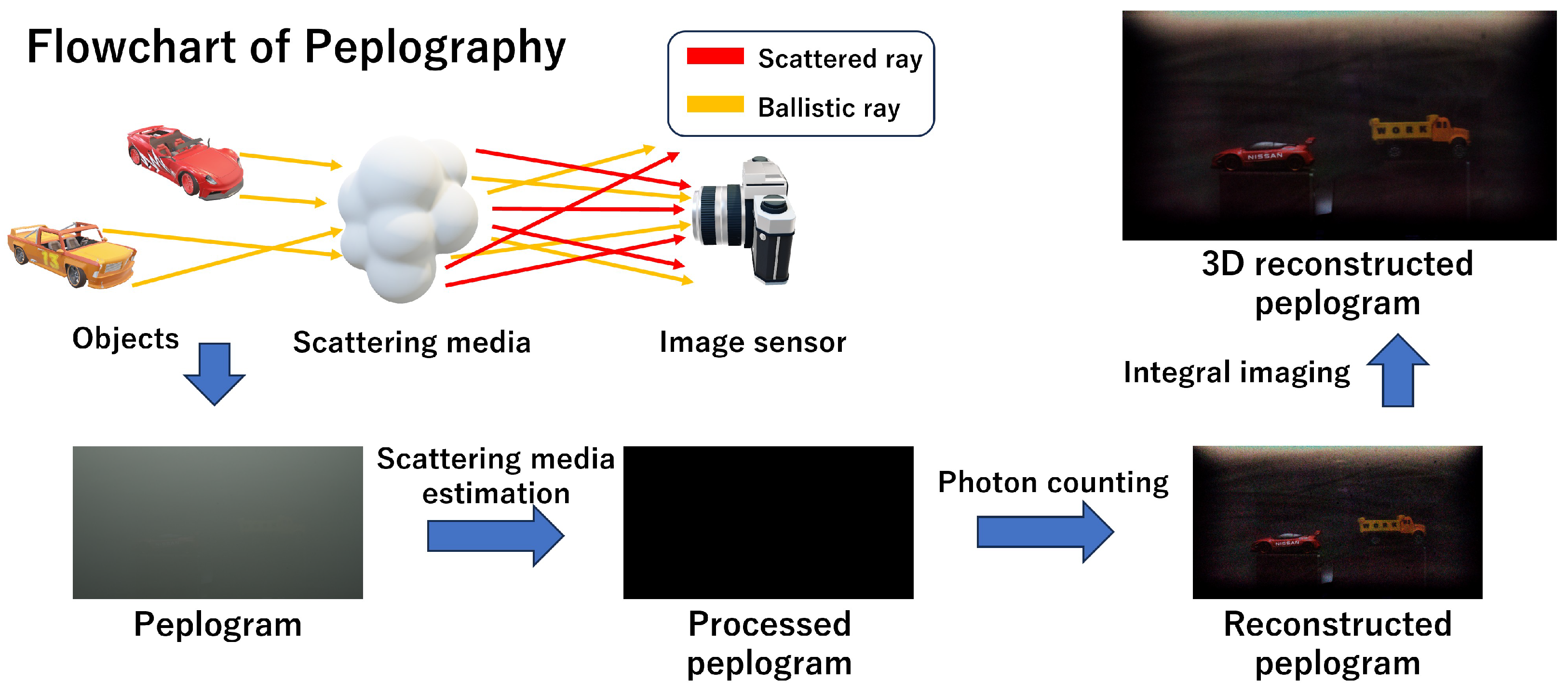
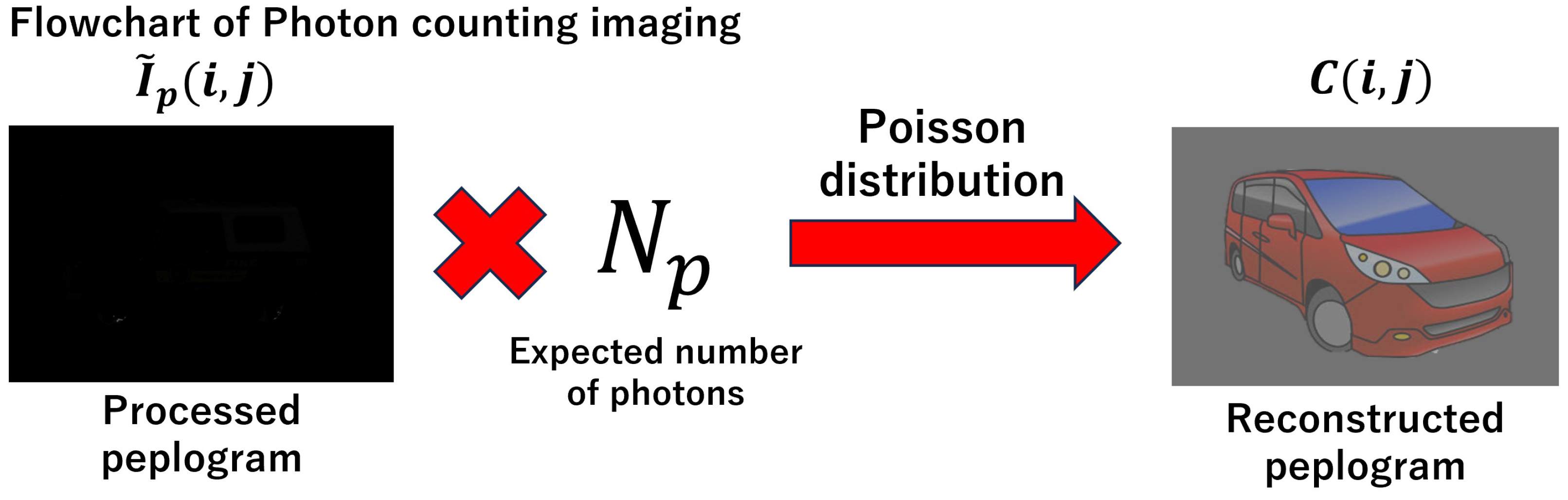
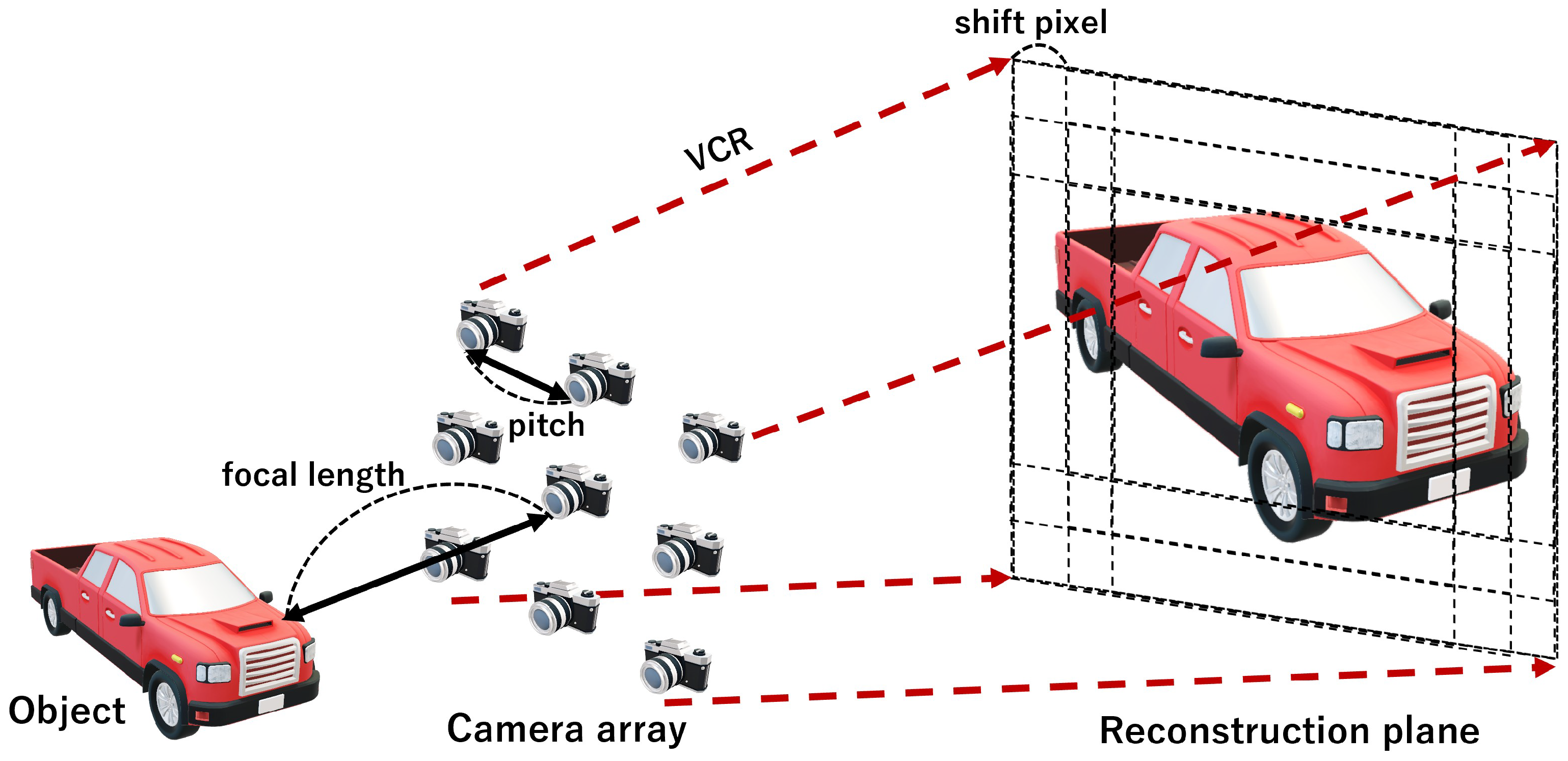
2.1. Peplography

Visualizing the object and obtaining its 3D information have been challenging for many fields such as autonomous driving systems and disaster situations. For this reason, many researchers have researched single image dehazing techniques and used artificial intelligence algorithms. However, these techniques may not obtain accurate details of the object in conditions of heavy scattering media. To solve this problem, peplography [14,15] has been proposed. Recorded images under heavy scattering media are called peplogram. Peplography can detect the photons of the objects from the single peplogram based on a statistical model and reconstruct a 3D peplogram using VCR [14,15]. Figure 1 illustrates the flowchart of peplography.

Peplography is divided into three steps, scattering media estimation, photon-counting algorithm, and 3D reconstruction. Scattering media can be estimated from the peplogram by maximum likelihood estimation (MLE) [14,15,16]. This is because the scattering media consists of the local scattering media with the size of the horizontal and the vertical ($w_x$, $w_y$), respectively. In addition, we can assume that the scattering media are Gaussian distribution with a mean ${\mu }_{ij}$ and a variance ${\sigma }_{ij}^2$ by central limit theorem, where i and j present the indices of each scattering media part in the x and y directions, respectively. Thus, the local scattering media part can be denoted as follows [14,15,16]:

$$\begin{array}{c}\hfill \begin{array}{cc}\hfill X_{ij}(m,n)=& I_p(i+m-1,j+n-1),\hfill \\ \hfill i=& 1,2,\dots ,N_x-w_x+1\hfill \\ \hfill j=& 1,2,\dots ,N_y-w_y+1\hfill \\ \hfill for\\ \hfill m=& 1,2,\dots ,w_x\hfill \\ \hfill n=& 1,2,\dots ,w_y\hfill \end{array}\end{array}$$

(1)

where $I_p$ represents the intensity of the pixels in the peplogram, $X_{ij}$ is the local scattering media part, and $N_x$, $N_y$ are the number of pixels of each peplogram, respectively. Gaussian distribution and the MLE are used to estimate the scattering media as [14,15]:

$$\begin{array}{c}\hfill \begin{array}{cc}\hfill & L\left(X_{ij}(m,n)\right|{\mu }_{ij},{\sigma }_{ij}^2)\hfill \\ \hfill & =\prod _{m=1}^{w_x}\prod _{n=1}^{w_y}{\displaystyle \frac{1}{\sqrt{2\pi {\sigma }^2}}}exp\left[-{\displaystyle \frac{{\{x_{ij}(m,n)-{\mu }_{ij}\}}^2}{2{\sigma }_{ij}^2}}\right]\hfill \\ \hfill & ={\displaystyle \frac{1}{\sqrt{2\pi {\sigma }^2}}}exp\left[-\sum _{m=1}^{w_x}\sum _{n=1}^{w_y}{\displaystyle \frac{{\{x_{ij}(m,n)-{\mu }_{ij}\}}^2}{2{\sigma }_{ij}^2}}\right]\hfill \end{array}\end{array}$$

(2)

To simplify the calculation, we take the logarithm of Equation (2). Then, we can obtain the equation below [14,15,16].

$$\begin{array}{c}\hfill \begin{array}{cc}\hfill & l\left\{x_{ij}(m,n)\right|{\mu }_{ij},{\sigma }_{ij}^2\}\hfill \\ \hfill & =ln\left({\displaystyle \frac{1}{\sqrt{2\pi {\sigma }^2}}}\right)-\sum _{m=1}^{w_x}\sum _{n=1}^{w_y}{\displaystyle \frac{{\{x_{ij}(m,n)-{\mu }_{ij}\}}^2}{2{\sigma }_{ij}^2}}\hfill \end{array}\end{array}$$

(3)

As a result, the scattering media can be estimated by the MLE as [14,15]:

$$\begin{array}{c}\hfill \begin{array}{cc}\hfill {\widehat{\mu }}_{ij}& =argmax\left\{x_{ij}(m,n)\right|{\mu }_{ij},{\sigma }_{ij}^2\}\hfill \\ \hfill & ={\displaystyle \frac{1}{w_x{w}_y}}\sum _{m=1}^{w_x}\sum _{n=1}^{w_y}{x}_{ij}(m,n)\hfill \end{array}\end{array}$$

(4)

From Equation (4), it is noticed that the estimated scattering media ${\widehat{\mu }}_{ij}$ is the mean of the local scattering media part ($w_x\times w_y$). By this statistical estimation from the peplogram, we can remove the scattering media from the peplogram as [14,15,16]:

$${\tilde{I}}_p(i,j)=I_p(i,j)-{\widehat{\mu }}_{ij}$$

(5)

where $I_p(i,j)$ represents the peplogram, ${\widehat{\mu }}_{ij}$ is the estimated scattering media, and ${\widehat{I}}_p(i,j)$ is the peplogram without scattering media (i.e., processed peplogram). Then, we use the photon-counting algorithm to detect the photons of the objects from the processed peplogram. The photon-counting algorithm is a method that can improve the visual quality of the images under photon-starved conditions by using statistical estimation. As we mentioned earlier, it follows Poisson distribution since the photons under photon-starved conditions occur rarely in unit time and space [26]. Therefore, Poisson distribution is used to detect the photons. In the processed peplogram, it seems to be recorded under photon-starved conditions. Thus, the photon-counting algorithm can be used to detect the photons from the processed peplogram. Figure 2 describes the flowchart of the photon-counting algorithm in peplography. The formula for detecting the photons of the objects is as follows [14]:

$$C_{ij}|{\widehat{I}}_p(i,j)\sim Poisson\left[{\gamma }_c{N}_p{\widehat{I}}_p(i,j)\right]$$

(6)

where $N_p$ is the number of photons describes from the processed peplogram, c is the index of color channels (R, G, and B), ${\gamma }_c$ is the coefficient of the photons from each color channel, and $C_{ij}$ is the reconstructed peplogram. Here, several photons can be extracted from a single pixel by multiplying the coefficient ${\gamma }_c{N}_p$ with the highest probability of Poisson distribution. Thus, the reconstructed peplogram can be obtained. The entire energy conveyed by the photons from the object behind the scattering media is proportional to the wavelength of the illumination [14]. Since each color channel has different wavelengths, different coefficients should be applied to the processed peplogram. The coefficients of the photons ${\gamma }_c$ can be defined with each color channel as [14]:

$${\gamma }_c={\displaystyle \frac{\eta }{h{\overline{v}}_c}}$$

(7)

where $\eta$ is the quantum efficiency which represents the average number of photoevents produced by each incident photon ($\eta \ge 1$), h is Plank’s constant, and ${\overline{v}}_c$ is the mean optical frequency of the radiation. We set the blue channel as the reference and the average wavelengths of each color channel are set to 685 nm (R: 620–750 nm), 532.5 nm (G: 495–570 nm), and 472.5 nm (B: 450–495 nm), respectively [14]. Thus, we can set the coefficients of the photons for each color channel to 1.4497, 1.1270, and 1, respectively.

However, the photon-counting algorithm may induce background noise and detect inaccurate photons in the peplogram. These effects degrade the visual quality of the images. To solve these problems and obtain accurate 3D information of objects, the integral imaging technique can be used. Integral imaging is a technique that can obtain 3D information of images using the lenslet array. However, using the lenslet array has the problem of low resolution [33]. Thus, we use a synthetic aperture integral imaging (SAII) method [30] which is one of the camera array-based pickup methods. We can obtain 3D information with high resolution by using SAII. It uses multiple 2D images which have different perspectives from the objects, and they are called the elemental images. In SAII, we use volumetric computational reconstruction (VCR) to generate 3D information of an object. Figure 3 illustrates the concept of the camera array method. VCR is one of the computational integral imaging reconstruction algorithms. It can obtain 3D information of objects by overlapping 2D elemental images which have different perspectives on the reconstruction plane. Moreover, VCR can enhance the visual quality of 3D images in the averaging process. The formula of VCR can be defined as follows [33]:

$$\Delta x={\displaystyle \frac{N_{x}pf}{c_x{z}_r}},\Delta y={\displaystyle \frac{N_{y}pf}{c_y{z}_r}}$$

(8)

$$R_c(x,y,z_r)={\displaystyle \frac{1}{N_{p}O(x,y,z_r)}}\sum _{k=0}^{K-1}\sum _{l=0}^{L-1}{C}_{(k,l)}(x+k\Delta x,y+l\Delta y)$$

(9)

where $\Delta x$, $\Delta y$ are the shift pixel value of each 2D elemental image, and $N_x$, $N_y$ are the number for the pixels of each elemental image in the x and y directions, respectively. In addition, p is the distance between the cameras, f is the focal length, $z_r$ is the reconstruction depth, and $c_x$, $c_y$ are the sensor size in the x and y directions, respectively. $C_{(k,l)}$ represents the reconstructed peplogram, $O(x,y,z_r)$ is the overlapping matrix at the reconstruction depth $z_r$, and $R_c(x,y,z_r)$ is the reconstructed 3D peplogram. The reconstructed 3D peplogram has better visual quality than the reconstructed 2D peplogram since the reconstructed 3D peplogram has less noise than the reconstructed 2D peplogram by conducting the averaging process in VCR. Therefore, conventional peplography can improve the visual quality of the images under heavy scattering media. However, the process of scattering media estimation is not automated. Figure 4 illustrates the concept of scattering media estimation in peplography.

In Equation (4), the scattering media information can be estimated by calculating the local mean of the scattering media part ($w_x\times w_y$). $w_x$ and $w_y$ mean the size of average filter and these values are not constant. Thus, finding the optimal filter size is necessary whenever the turbidity of the single peplogram is changed. To solve this problem, in this paper, we propose a new method of scattering media estimation.

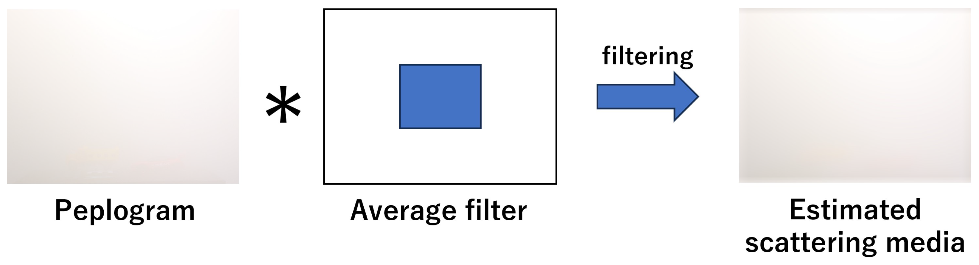
2.2. Proposed Method

To automate the process of the scattering media estimation in peplography, we suggest a novel estimation technique utilizing the singular value decomposition (SVD) and the discrete cosine transform (DCT). SVD is a method with which an arbitrary m × n matrix can be decomposed into three matrices, $U,\Sigma ,V^T$, as shown in Figure 5 [36]. In addition, Figure 5 can be described as:

$$\begin{array}{c}\hfill \begin{array}{cc}\hfill Y_n=X_n& +Z_n\hfill \\ \hfill Y_n=\sum _{i=1}^n{y}_{n,i}{u}_{n,i}{v}_{n,i}^T,& X_n=\sum _{i=1}^r{x}_i{u}_{n,i}{v}_{n,i}^T\hfill \end{array}\end{array}$$

(10)

where $Y_n$ is the decomposed data of the arbitrary m × n matrix using SVD, $X_n$ is the unknown $m\times n$ matrix thought to be either exactly or approximately of the low rank which has the primary information of the matrix $Y_n$, and $Z_n$ is the noise matrix which is statistically independent of the $X_n$ matrix. $y_{n,i}$ is the singular value matrix of $Y_n$, $u_{n,i}$ is the left singular vector matrix of $Y_n$, $v_{n,i}^T$ is the right singular vector matrix of $Y_n$, r is the estimated rank of $X_n$, and $x_i$ is the vector of the singular values, which means the primary signal information of the matrix, respectively. However, since the $X_n$ is an unknown matrix that we need to estimate, we can only check the matrix $Y_n$ containing the noise matrix $Z_n$ [37,38]. To remove the noise matrix, we can truncate the singular value matrix at the bulk edge because the noise information $Z_n$ is removed asymptotically if $Z_n$ is closer to the bulk edge [38]. The bulk edge of the singular value represents the boundary line that indicates the presence or absence of noise. The bulk edge of the singular value is located approximately at 2 and the location of the bulk edge can be shown as [37]:

$$Locationofthebulkedge=X_{i,i}+{\displaystyle \frac{1}{X_{i,i}}}(i=1,2)$$

(11)

where $X_{i,i}$ is the index of the vector for the singular value $X_n$. And this equation can be proved as [37]:

$$\begin{array}{c}\hfill \begin{array}{cc}\hfill & for1\le i\le r\hfill \\ \hfill \beta ={\displaystyle \frac{n}{m}}& (m\ne n,m\ge n)\hfill \\ \hfill \underset{n\to \infty }{lim}{y}_{n,i}\approx & \left\{\begin{array}{cc}\sqrt{(x_i+{\displaystyle \frac{1}{x_i}})(x_i+{\displaystyle \frac{\beta }{x_i}})}\hfill & x_i>{\beta }^{{\displaystyle \frac{1}{4}}}\hfill \\ 1+\sqrt{\beta }\hfill & x_i\le {\beta }^{{\displaystyle \frac{1}{4}}}\hfill \end{array}\right.\hfill \end{array}\end{array}$$

(12)

where $\beta$ is the height–width ratio of the matrix. Thus, the noise information $Z_n$ can be removed by truncating the singular values to the bulk edge. In the single peplogram, the scattering media is the primary information of the single peplogram and the object can be assumed to be noise information. Therefore, we can estimate the scattering media which do not have the noise information by truncating the singular value matrix at the bulk edge.

DCT is a method that can transform the spatial domain into frequency domain, and it can be applied to 2D images to obtain the frequency information of the image [39,40]. Figure 6 describes the concept of DCT. In addition, the formula for DCT is as follow [39,40]:

$$\begin{array}{c}\hfill \begin{array}{cc}\hfill u=0,\dots ,M-1& v=0,\dots ,N-1\hfill \\ \hfill F(u,v)=a\left(u\right)a\left(v\right)\sum _{x=0}^{M-1}\sum _{y=0}^{N-1}& f(x,y)cos\left[{\displaystyle \frac{\pi (2x+1)u}{2M}}\right]cos\left[{\displaystyle \frac{\pi (2y+1)v}{2N}}\right]\hfill \\ \hfill a\left(u\right)=\left\{\begin{array}{c}{\displaystyle \frac{1}{\sqrt{M}}}ifu=0\hfill \\ {\displaystyle \frac{2}{\sqrt{M}}}if1\le u\le M-1\hfill \end{array}\right.& anda\left(v\right)=\left\{\begin{array}{c}{\displaystyle \frac{1}{\sqrt{N}}}ifv=0\hfill \\ {\displaystyle \frac{2}{\sqrt{N}}}if1\le v\le N-1\hfill \end{array}\right.\hfill \end{array}\end{array}$$

(13)

where $F(u,v)$ is the transformed image by DCT, M and N are the number of pixels in the x and y directions, respectively, and $f(x,y)$ is a 2D image. In Figure 6, it has the high-frequency component as it goes down to the bottom right and the white pixel means the direct current (DC) component. In DCT, since it has the primary information about the image in the DC component and the low frequency area, the primary information of the image can be obtained by implementing the low-pass filter in the frequency domain. This method is used in most digital image-processing techniques such as JPEG [40]. In peplography, the primary information of the image means the scattering media as we mentioned earlier. Thus, we can estimate the scattering media using this method.

The proposed method uses these two methods since these two methods can only obtain the scattering media information. As shown in Figure 7, the flowchart illustrates our proposed method.

In Figure 7, ISVD and IDCT are inverse SVD and inverse DCT, respectively. First, DCT is used to transform the single peplogram into the frequency domain and use SVD to decompose the primary information. When we use SVD in the spatial domain, it can cause image distortion. Thus, DCT can be used to solve this problem since the spatial domain can be transformed into the frequency domain by DCT to prevent the image distortion when applying SVD. In addition, DCT is suitable for using SVD since the result of DCT comes out in an integer. The equation of this process is:

$$R(u,v)=a\left(u\right)a\left(v\right)\sum _{y=0}^{M-1}\sum _{x=0}^{N-1}r(x,y)cos\left[{\displaystyle \frac{\pi (2x+1)u}{2M}}\right]cos\left[{\displaystyle \frac{\pi (2y+1)v}{2N}}\right]$$

(14)

$$R(u,v)=\sum _{i=1}^n{r}_{n,i}{u}_{n,i}{v}_{n,i}^T$$

(15)

where $R(u,v)$ is the transformed single peplogram in the frequency domain, $r(x,y)$ is the single peplogram in the spatial domain, and $r_{n,i}$ is the singular value matrix of $R(u,v)$. Then, we truncate the singular value matrix at the bulk edge to remove the noise information and obtain the only scattering media information. The equation of this process is:

$$\sum _{i=1}^2{r}_{2,i}{u}_{2,i}{v}_{2,i}^T=R^{\prime }(u,v)$$

(16)

where $R^{\prime }(u,v)$ is the reconstructed frequency domain of the transformed single peplogram. As we mentioned earlier, the bulk edge is approximately 2. Therefore, we truncate the singular value matrix at 2. However, this method is not sufficient to estimate the accurate scattering media information and still can induce the image distortion. As we mentioned before, the scattering media information can also be obtained by applying the low-pass filter in the frequency domain. Thus, a Gaussian low-pass filter is used to estimate the accurate scattering media information and prevent image distortion. The process of this equation is:

$$\begin{array}{c}\hfill \begin{array}{cc}\hfill G(x,y)& ={\displaystyle \frac{1}{2\pi {\sigma }^2}}exp\left(-{\displaystyle \frac{x^2+y^2}{2{\sigma }^2}}\right)\hfill \\ \hfill S(u,v)& =R^{\prime }(u,v)\times G(x,y)\hfill \end{array}\end{array}$$

(17)

where $G(x,y)$ is Gaussian low-pass filter, and $S(u,v)$ is the result of the filtering process. The scattering media information can be obtained from a peplogram by estimating scattering media information two times with a truncating process and filtering with a Gaussian low-pass filter. Finally, IDCT can be applied to automatic estimation of the scattering media. The equation of this process is:

$$s(x,y)=\sum _{u=0}^{M-1}\sum _{v=0}^{N-1}a\left(u\right)a\left(v\right)S(u,v)cos\left[{\displaystyle \frac{\pi (2x+1)u}{2M}}\right]cos\left[{\displaystyle \frac{\pi (2y+1)v}{2N}}\right]$$

(18)

where $s(x,y)$ is the estimated scattering media information using our proposed method. We can recognize that the equations of the proposed method do not have a value to change. As a result, we can automate the process of estimating scattering media information.

3. Experimental Setup and Results

Experimental Setup

To record the elemental images under conditions of scattering media, we used 5(H) × 5(V) camera arrays and we made the camera array using the “Nikon D850” camera and the “AF-P NIKKOR 70–300 mm 1:4.5-6.3G ED” lens. We set the real scattering media using the fog machine (FM01, Ulanzi) in the tank with size 600 mm (W) × 450 mm (D) × 450 mm (H). In this scattering media environment, the focal length of each camera is 70 mm and the pitch between cameras is 2 mm. The sensor size of each camera is 36 mm (H) × 24 mm (V) and the resolution of each elemental image is 1920 (H) × 1080 (V). In addition, the ISO of each camera is 100, and the exposure time of each camera is 1.6 s. Figure 8 illustrates the experimental setup of the scattering media environment.

In this experiment, we gradually inject fog into the glass tank until the scene appears to be under heavy scattering media conditions. We also irradiate approximately 5 W power of light using a light source (BL2-0808WHIIC, Advanced Illumination, Rochester, VT, USA) when we conducted the experiment since we demonstrated the heavy scattering media conditions in the normal light environment. Figure 9 shows the reference image and the single 2D peplogram under a scattering media situation with normal light conditions.

Then, the result of the conventional method is compared with our proposed method. Figure 10 and Figure 11 show the result of the yellow truck and the orange car.

In Figure 10 and Figure 11, the result of the conventional method is the best result that uses the optimal filter size 800 × 600, $N_p$ is 7000 and the depth is 474 mm and 504 mm, respectively. Since the optimal filter size can be found manually, it takes too much time to find the optimal filter size of various real-world images. In contrast, our proposed method does not need to control any values manually. We can see that the result by our proposed method is almost the same as the result by the optimal conventional method. Thus, the process of estimating scattering media information can be automated by our proposed method. In addition, it can obtain the optimal result of the conventional peplography. For comparison of the numerical analysis of each method, we use various image quality-assessment (IQA) methods such as structural similarity (SSIM), feature similarity (FSIMc), gradient magnitude similarity deviation (GMSD), and learned perceptual image path similarity (LPIPS) [41,42,43]. SSIM and FSIM mean better performance when the numerical value is close to 1. In contrast, GMSD and LPIPS mean better performance when the numerical value is close to 0. The numerical value of each method is shown in Figure 12 with various IQA methods.

In Figure 12, it is denoted that our proposed method shows similar performance to the optimal conventional method in various IQA metrics. This verifies that the proposed method can automatically acquire the optimal result of the conventional peplography. Furthermore, to verify the applicability of our proposed method under various conditions, we conduct another experiment that changes the number of objects and the resolution of each elemental image. Figure 13 shows the reference image and the single 2D peplogram which has changed conditions.

We used three different objects in this experiment and set the resolution of each elemental image to 2200 (H) × 1600 (V). Figure 14, Figure 15 and Figure 16 show the result of a yellow truck where it is located at 616 mm, a red car where it is located at 631 mm, and an orange car where it is located at 676 mm, respectively. In Figure 14, Figure 15 and Figure 16, we changed the filter size to 400 (H) × 300 (V) to obtain the optimal result in the conventional method. In contrast, our proposed method can obtain the optimal result without any manual control. As shown in Figure 17, our proposed method produces results similar to the optimal results of the conventional method. We can confirm that the result of each IQA method has similar values. Therefore, our proposed method can automate the conventional method in various conditions. Furthermore, our proposed method can obtain the optimal results by the conventional method in various conditions.

4. Conclusions

In this paper, we have proposed a new method that can automate the scattering media-estimation process. The conventional peplography has the problem that it cannot be used in real-world situations because the process of estimating scattering media information in peplography requires changing the filter size when the peplogram is changed. To overcome this problem, we have proposed a new method of estimating scattering media information using singular value decomposition (SVD) and discrete cosine transform (DCT). Since SVD and DCT can obtain the only scattering media information from the single peplogram, it can estimate the scattering media information automatically. In addition, to verify our proposed method, we experimented with two different conditions and calculated the numerical analysis value using various image quality-assessment (IQA) methods such as structural similarity (SSIM), feature similarity (FSIMc), gradient magnitude similarity deviation (GMSD), and learned perceptual image patch similarity (LPIPS). As a result, in the experiment using two objects, our proposed method has been able to automate the conventional peplography. Furthermore, it has been able to obtain the optimal result by the conventional peplography. In another experiment, we changed the number of objects and the resolution of each elemental image to verify our proposed method can be applied in various situations. As a result, even though the conventional peplography requests the optimization of the filter size to obtain the optimal result, our proposed method can obtain the optimal result automatically in different situations. We believe that our proposed method can contribute to enhancing the technology of autonomous driving, disaster situations, astrophotography, and overall industrial fields. In particular, our proposed method can contribute to technologies such as autonomous driving in scattering media conditions and lifesaving in fire disasters. Moreover, we can use artificial intelligence (AI) technology in our proposed method if we have sufficient datasets for scattering media situations. AI technology such as supervised learning can extract the features of objects and scattering media. Thus, it can be used for improving the performance of estimation of scattering media information. However, our proposed method has limitations such as background and real-time processing. When the background is bright or white, our proposed method is unable to obtain the object information accurately. In addition, the conventional peplography is capable of real-time processing [16]. However, the processing speed of our proposed method is slower than the conventional peplography by approximately 70%. Therefore, we will research using an AI model to improve the performance of scattering media estimation and optimize peplography to solve the background problem for future work. Furthermore, we aim to improve the speed of the computational process to make our proposed method suitable for real-time processing.

References

1. Liu, J.; Wang, S.; Wang, X.; Ju, M.; Zhang, D. A review of remote sensing image dehazing. Sensors 2021, 21, 3926. [Google Scholar] [CrossRef] [PubMed]
2. Tan, Y.; Zhu, Y.; Huang, Z.; Tan, H.; Chang, W. Brief Industry Paper: Real-Time Image Dehazing for Automated Vehicles. In Proceedings of the 2023 IEEE Real-Time Systems Symposium (RTSS), Taipei, Taiwan, 5–8 December 2023; IEEE: Piscataway, NJ, USA, 2023; pp. 478–483. [Google Scholar]
3. Wang, Y.; Chao, W.L.; Garg, D.; Hariharan, B.; Campbell, M.; Weinberger, K.Q. Pseudo-lidar from visual depth estimation: Bridging the gap in 3d object detection for autonomous driving. In Proceedings of the IEEE/CVF Conference on Computer Vision and Pattern Recognition (CVPR), Long Beach, CA, USA, 15–20 June 2019; pp. 8445–8453. [Google Scholar]
4. Li, Y.; Ibanez-Guzman, J. Lidar for autonomous driving: The principles, challenges, and trends for automotive lidar and perception systems. IEEE Signal Process. Mag. 2020, 37, 50–61. [Google Scholar] [CrossRef]
5. Schechner, Y.Y.; Narasimhan, S.G.; Nayar, S.K. Instant dehazing of images using polarization. In Proceedings of the 2001 IEEE Computer Society Conference on Computer Vision and Pattern Recognition (CVPR), Kauai, HI, USA, 8–14 December 2001; IEEE: Piscataway, NJ, USA, 2001; Volume 1, p. 1. [Google Scholar]
6. He, K.; Sun, J.; Tang, X. Single image haze removal using dark channel prior. IEEE Trans. Pattern Anal. Mach. Intell. 2010, 33, 2341–2353. [Google Scholar] [PubMed]
7. Zhu, Q.; Mai, J.; Shao, L. A fast single image haze removal algorithm using color attenuation prior. IEEE Trans. Image Process. 2015, 24, 3522–3533. [Google Scholar]
8. Cai, B.; Xu, X.; Jia, K.; Qing, C.; Tao, D. Dehazenet: An end-to-end system for single image haze removal. IEEE Trans. Image Process. 2016, 25, 5187–5198. [Google Scholar] [CrossRef]
9. Zhang, H.; Sindagi, V.; Patel, V.M. Multi-scale single image dehazing using perceptual pyramid deep network. In Proceedings of the IEEE Conference on Computer Vision and Pattern Recognition Workshops (CVPRW), Salt Lake City, UT, USA, 14–19 June 2018; pp. 902–911. [Google Scholar]
10. Dong, H.; Pan, J.; Xiang, L.; Hu, Z.; Zhang, X.; Wang, F.; Yang, M.H. Multi-Scale Boosted Dehazing Network With Dense Feature Fusion. In Proceedings of the IEEE/CVF Conference on Computer Vision and Pattern Recognition (CVPR), Virtual, 14–19 June 2020; pp. 2157–2167. [Google Scholar]
11. Agrawal, S.C.; Jalal, A.S. A comprehensive review on analysis and implementation of recent image dehazing methods. Arch. Comput. Methods Eng. 2022, 29, 4799–4850. [Google Scholar] [CrossRef]
12. Wang, Y.; Yan, X.; Wang, F.L.; Xie, H.; Yang, W.; Zhang, X.P.; Qin, J.; Wei, M. Ucl-dehaze: Towards real-world image dehazing via unsupervised contrastive learning. IEEE Trans. Image Process. 2024, 33, 1361–1374. [Google Scholar] [CrossRef] [PubMed]
13. Wang, X.; Fu, W.; Yu, H.; Zhang, Y. Effective polarization-based image dehazing through 3D convolution network. Signal Image Video Process. 2024, 18 (Suppl. S1), 1–12. [Google Scholar] [CrossRef]
14. Cho, M.; Javidi, B. Peplography—A passive 3D photon counting imaging through scattering media. Opt. Lett. 2016, 41, 5401–5404. [Google Scholar] [CrossRef] [PubMed]
15. Lee, J.; Cho, M.; Lee, M.C. 3D visualization of objects in heavy scattering media by using wavelet peplography. IEEE Access 2022, 10, 134052–134060. [Google Scholar] [CrossRef]
16. Ono, S.; Kim, H.W.; Cho, M.; Lee, M.C. A research on scattering removal technology using compact GPU machine for real-time visualization. In Proceedings of the 2023 23rd International Conference on Control, Automation and Systems (ICCAS), Yeosu, Republic of Korea, 17–20 October 2023; IEEE: Piscataway, NJ, USA, 2023; pp. 1460–1464. [Google Scholar]
17. Tavakoli, B.; Javidi, B.; Watson, E. Three dimensional visualization by photon counting computational integral imaging. Opt. Express 2008, 16, 4426–4436. [Google Scholar] [CrossRef] [PubMed]
18. Moon, I.; Javidi, B. Three-dimensional recognition of photon-starved events using computational integral imaging and statistical sampling. Opt. Lett. 2009, 34, 731–733. [Google Scholar] [CrossRef]
19. Aloni, D.; Stern, A.; Javidi, B. Three-dimensional photon counting integral imaging reconstruction using penalized maximum likelihood expectation maximization. Opt. Express 2011, 19, 19681–19687. [Google Scholar] [CrossRef] [PubMed]
20. Xiao, X.; Javidi, B. 3D photon counting integral imaging with unknown sensor positions. JOSA A 2012, 29, 767–771. [Google Scholar] [CrossRef]
21. Lee, C.G.; Moon, I.; Javidi, B. Photon-counting three-dimensional integral imaging with compression of elemental images. JOSA A 2012, 29, 854–860. [Google Scholar] [CrossRef] [PubMed]
22. Jung, J.; Cho, M.; Dey, D.K.; Javidi, B. Three-dimensional photon counting integral imaging using Bayesian estimation. Opt. Lett. 2010, 35, 1825–1827. [Google Scholar] [CrossRef]
23. Kim, H.W.; Lee, M.C.; Cho, M. Three-Dimensional Image Visualization under Photon-Starved Conditions Using N Observations and Statistical Estimation. Sensors 2024, 24, 1731. [Google Scholar] [CrossRef] [PubMed]
24. Morton, G. Photon counting. Appl. Opt. 1968, 7, 1–10. [Google Scholar] [CrossRef]
25. Srinivas, M.D.; Davies, E.B. Photon counting probabilities in quantum optics. Int. J. Opt. 1981, 28, 981–996. [Google Scholar] [CrossRef]
26. Goodman, J.W. Statistical Optics; John Wiley & Sons: Hoboken, NJ, USA, 2015. [Google Scholar]
27. Watson, E.A.; Morris, G.M. Comparison of infrared upconversion methods for photon-limited imaging. J. Appl. Phys. 1990, 67, 6075–6084. [Google Scholar] [CrossRef]
28. Tsuchiya, Y.; Inuzuka, E.; Kurono, T.; Hosoda, M. Photon-counting imaging and its application. In Advances in Electronics and Electron Physics; Elsevier: Amsterdam, The Netherlands, 1986; Volume 64, pp. 21–31. [Google Scholar]
29. Lippmann, G. La photographie integrale. Comptes-Rendus 1908, 146, 446–451. [Google Scholar]
30. Jang, J.S.; Javidi, B. Three-dimensional synthetic aperture integral imaging. Opt. Lett. 2002, 27, 1144–1146. [Google Scholar] [CrossRef] [PubMed]
31. Hong, S.H.; Jang, J.S.; Javidi, B. Three-dimensional volumetric object reconstruction using computational integral imaging. Opt. Express 2004, 12, 483–491. [Google Scholar] [CrossRef] [PubMed]
32. Park, J.H.; Hong, K.; Lee, B. Recent progress in three-dimensional information processing based on integral imaging. Appl. Opt. 2009, 48, H77–H94. [Google Scholar] [CrossRef] [PubMed]
33. Javidi, B.; Carnicer, A.; Arai, J.; Fujii, T.; Hua, H.; Liao, H.; Martínez-Corral, M.; Pla, F.; Stern, A.; Waller, L.; et al. Roadmap on 3D integral imaging: Sensing, processing, and display. Opt. Express 2020, 28, 32266–32293. [Google Scholar] [CrossRef]
34. Lee, J.; Usmani, K.; Javidi, B. Polarimetric 3D integral imaging profilometry under degraded environmental conditions. Opt. Express 2024, 32, 43172–43183. [Google Scholar] [CrossRef]
35. Inoue, K.; Cho, M. Visual quality enhancement of integral imaging by using pixel rearrangement technique with convolution operator (CPERTS). Opt. Lasers Eng. 2018, 111, 206–210. [Google Scholar] [CrossRef]
36. Kahu, S.; Rahate, R. Image compression using singular value decomposition. Int. J. Adv. Res. Technol. 2013, 2, 244–248. [Google Scholar]
37. Gavish, M.; Donoho, D.L. The optimal hard threshold for singular values is 4/√3. IEEE Trans. Inf. Theory 2014, 60, 5040–5053. [Google Scholar] [CrossRef]
38. Donoho, D.; Gavish, M.; Romanov, E. ScreeNOT: Exact MSE-optimal singular value thresholding in correlated noise. Ann. Stat. 2023, 51, 122–148. [Google Scholar] [CrossRef]
39. Pascal, N.; Ele, P.; Basile, K.I. Compression approach of EMG signal using 2D discrete wavelet and cosine transforms. Am. J. Signal Process. 2013, 3, 10–16. [Google Scholar]
40. Raid, A.; Khedr, W.; El-Dosuky, M.A.; Ahmed, W. Jpeg image compression using discrete cosine transform-A survey. arXiv 2014, arXiv:1405.6147. [Google Scholar]
41. Zhang, L.; Zhang, L.; Mou, X.; Zhang, D. FSIM: A feature similarity index for image quality assessment. IEEE Trans. Image Process. 2011, 20, 2378–2386. [Google Scholar] [CrossRef]
42. Xue, W.; Zhang, L.; Mou, X.; Bovik, A.C. Gradient magnitude similarity deviation: A highly efficient perceptual image quality index. IEEE Trans. Image Process. 2013, 23, 684–695. [Google Scholar] [CrossRef]
43. Zhang, R.; Isola, P.; Efros, A.A.; Shechtman, E.; Wang, O. The unreasonable effectiveness of deep features as a perceptual metric. In Proceedings of the IEEE Conference on Computer Vision and Pattern Recognition (CVPR), Salt Lake City, UT, USA, 18–22 June 2018; pp. 586–595. [Google Scholar]
Figure 1. Flowchart of peplography.
Electronics 14 00545 g001
Figure 2. Flowchart of photon-counting algorithm in peplography.
Electronics 14 00545 g002
Figure 3. Concept of the camera array-based pickup method.
Electronics 14 00545 g003
Figure 4. Concept of scattering media estimation in peplography, where ∗ represents a convolution operator.
Electronics 14 00545 g004
Figure 5. Singular value decomposition (SVD).
Electronics 14 00545 g005
Figure 6. Concept of the discrete cosine transform (DCT).
Electronics 14 00545 g006
Figure 7. Flowchart of the proposed method.
Electronics 14 00545 g007
Figure 8. Experiment setup of the scattering media environment.
Electronics 14 00545 g008
Figure 9. Scattering media situations. (a) Reference image and (b) 2D single peplogram.
Electronics 14 00545 g009
Figure 10. Reconstructed 3D images. (a) Reference image, (b) single peplogram, (c) reconstructed 3D image by the conventional peplography, and (d) reconstructed 3D image by our proposed method where the depth is 474 mm.
Electronics 14 00545 g010
Figure 11. Reconstructed 3D images. (a) Reference image, (b) single peplogram, (c) reconstructed 3D image by the conventional peplography, and (d) reconstructed 3D image by our proposed method where the depth is 504 mm.
Electronics 14 00545 g011
Figure 12. Results of each IQA method.
Electronics 14 00545 g012
Figure 13. Experiment under changed conditions. (a) Reference image and (b) 2D single peplogram.
Electronics 14 00545 g013
Figure 14. Reconstructed 3D images. (a) Reference image, (b) single peplogram, (c) reconstructed 3D image by the conventional peplography, and (d) reconstructed 3D image by our proposed method, where the depth is 616 mm.
Electronics 14 00545 g014
Figure 15. Reconstructed 3D images. (a) Reference image, (b) single peplogram, (c) reconstructed 3D image by the conventional peplography, and (d) reconstructed 3D image by our proposed method, where the depth is 631 mm.
Electronics 14 00545 g015
Figure 16. Reconstructed 3D images. (a) Reference image, (b) single peplogram, (c) reconstructed 3D image by the conventional peplography, and (d) reconstructed 3D image by our proposed method, where the depth is 676 mm.
Electronics 14 00545 g016
Figure 17. Results of each IQA method.
Electronics 14 00545 g017
Disclaimer/Publisher’s Note: The statements, opinions and data contained in all publications are solely those of the individual author(s) and contributor(s) and not of MDPI and/or the editor(s). MDPI and/or the editor(s) disclaim responsibility for any injury to people or property resulting from any ideas, methods, instructions or products referred to in the content.