Advancing Multi-Label Tomato Leaf Disease Identification Using Vision Transformer and EfficientNet with Explainable AI Techniques

Abstract

Plant diseases pose a significant threat to global food security, affecting crop yield, quality, and overall agricultural productivity. Traditionally, diagnosing plant diseases has relied on time-consuming visual inspections by experts, which can often lead to errors. Machine learning (ML) and artificial intelligence (AI), particularly Vision Transformers (ViTs), and Convolutional Neural Networks, offer a faster, automated alternative for identifying plant diseases through leaf image analysis. However, these models are often criticized for their “black box” nature, limiting trust in their predictions due to a lack of transparency. Our findings show that incorporating Explainable AI (XAI) techniques, such as Grad-CAM, Integrated Gradients, and LIME, significantly improves model interpretability, making it easier for practitioners to identify the underlying symptoms of plant diseases. This study not only contributes to the field of plant disease detection but also offers a novel perspective on improving AI transparency in real-world agricultural applications through the use of XAI techniques. With training accuracies of 100.00% for ViT, 96.88% for EfficientNetB7, 93.75% for EfficientNetB0, and 87.50% for ResNet50, and corresponding validation accuracies of 96.39% for ViT, 86.98% for EfficientNetB7, and 82.00% for EfficientNetB0, our proposed models outperform earlier research on the same dataset. This demonstrates a notable improvement in model performance while maintaining transparency and trustworthiness through interpretable and reliable decision-making.

1. Introduction

Agriculture plays a fundamental role in feeding the growing global population, yet it faces significant challenges from plant diseases that affect crop yield, quality, and overall productivity. As the world’s population continues to rise, food security is increasingly threatened by these diseases. Traditionally, the identification and diagnosis of plant diseases have been carried out through manual inspection by agricultural experts, a process that is often labor intensive, time consuming, and prone to human error [1]. With the development of machine learning (ML) and artificial intelligence (AI), opportunities to automate plant disease diagnosis have emerged, offering the potential to increase both the speed and accuracy of disease detection while reducing human intervention.

Among AI techniques, Vision Transformers (ViTs) and Convolutional Neural Networks (CNNs), two families of deep learning models, have shown exceptional promise for diagnosing plant diseases through the analysis of leaf images. Since plant leaves are often the primary indicators of disease, their visual symptoms, such as discoloration, irregular textures, and stains, serve as critical clues for disease detection [2]. CNNs are particularly effective at image classification tasks, enabling automated systems to process large datasets of leaf images and detect disease symptoms without manual involvement [2]. However, while CNN models excel at classification, they are often criticized as “black box” models, meaning that the decision-making process behind their predictions is not transparent. In applications like plant disease detection, where trust and understanding are crucial, this lack of interpretability can be a significant barrier to widespread adoption. To address this issue, Explainable AI (XAI) has been introduced as a solution. XAI methods aim to make the decision-making process of AI models more transparent and understandable by providing explanations of how models arrive at their conclusions. In the context of plant disease diagnosis, integrating XAI with CNN models can enhance trust in the system by clearly identifying which features of the leaf images contributed to the model’s predictions. By improving transparency, XAI can not only help users better understand the underlying symptoms of the diseases but also foster collaboration between agronomists, farmers, and AI researchers to develop more reliable and context-aware disease detection technologies.

This research builds on previous studies in plant disease detection using deep learning, aiming to make a meaningful contribution by addressing the challenges of multi-label classification. While most existing work focuses on multiclass classification, assigning a single disease category to a plant leaf, real-world scenarios often involve plants suffering from multiple diseases simultaneously. To bridge this gap, this research explores multi-label disease detection, enabling the diagnosis of multiple diseases from a single-leaf image. In particular, this work seeks to enhance the training and testing accuracy of multi-label models, ensuring more robust and reliable predictions even in the presence of limited or noisy datasets. Additionally, this work integrates XAI techniques to improve the interpretability of these models, offering insights into how AI systems identify and differentiate between various diseases. By improving both the accuracy and transparency of the models, this approach not only strengthens the reliability of plant disease diagnosis but also fosters greater trust in AI-driven solutions for agriculture. Through this work, we aim to address the technical challenges of multi-label plant disease detection, including improving training accuracy, while meeting the critical need for transparency in AI models. Ultimately, this research aspires to advance agricultural technology by providing more effective, interpretable, and trustworthy solutions for disease management. These aspects, multi-label classification and integrated XAI, remain underexplored in prior work and represent the key gaps addressed in this study.

The rest of the paper is structured as follows: Section 2 covers related work, Section 3 details the methodology, Section 4 presents results and analysis, and Section 5 concludes the study.

2. Related Works

Recent developments in ML and AI have created new opportunities to automate disease diagnosis, especially in the agriculture sector [2]. Deep learning models like ViTs and CNNs, are among these developments. They are excellent tools for diagnosing plant diseases from leaf photos because they have shown improved performance in the task of image classification.

Plant leaves are one of the main indicators of disease because they often exhibit most symptoms, which can range from irregular textures to discolorations and stains. By processing massive datasets of leaf pictures, automated systems utilizing CNNs can analyze these symptoms without the need for manual examination. CNN models are excellent at categorization, but are sometimes referred to as “black-box” models because it is difficult to understand how they make decisions [2]. In high-stakes applications like agriculture, where agronomists and farmers must trust the system’s forecasts before taking corrective action, this lack of transparency poses difficulties.

Explainable AI (XAI) is the answer to this issue as it provides information about the methods and rationale behind a model’s decision-making. By emphasizing the areas of leaf images that contribute the most to the model’s predictions, integrating XAI approaches with CNN models can improve transparency and trust in the context of plant disease diagnosis [3]. This helps users to better understand the underlying symptoms of the condition and also helps to increase the system’s reliability. Moreover, explainable models can help agricultural specialists and AI researchers collaborate to create more reliable and contextually aware disease detection technologies. A great deal of research has already been carried out on plant disease detection, as described in the following literature review.

In the research of Chowdhury et al. [4], they applied a deep learning design built on the latest EfficientNet convolutional neural network on 18,161 plain and tomato infections using segmented photos of tomato leaves. They developed two models for the segmentation of leaves, namely, U-net and Modified U-net. They presented the analogous performance of the six-class and binary classification models (healthy and unhealthy leaves) (healthy and diverse groupings of unhealthy leaves), as well as a ten-class system (healthy and diverse kinds of poor foliage) have also been introduced. The U-net segmentation model revealed accuracy, IoU, and Dice score for the division of the data were 98.66%, 98.50%, and 98.73%, respectively.

To enhance the information extracted from the photos, pixel-based techniques were implemented on the processed images of infected leaves in the study of Panchal et al. [5]. Next, feature extraction was carried out, then image segmentation, and finally, crop disease classification based on the patterns identified from the affected leaves. CNNs are used to classify diseases. A public dataset comprising around 87,000 RGB photos, containing both healthy and diseased leaves, was used for demonstration purposes. At its peak, it outperformed current validation data with an accuracy of 93.5%, making their model the new standard for more extensive classification.

A study by Liu et al. [6] proposed a recognition approach that was based on convolutional neural networks for the diagnoses of grape leaf diseases. A data set of 107,366 grape leaf images was generated via image enhancement techniques. Afterward, inception structure was applied for strengthening the performance of multidimensional feature extraction. A dense connectivity strategy was introduced to encourage feature reuse and strengthen feature propagation. Ultimately, the model was built and trained from scratch. The overall accuracy was 97.22% for the test set.

Another research article by Liu et al. [7], proposed an accurate identification approach for apple leaf diseases based on deep CNNs. The researcher uses pathological images and designed an architecture of a deep convolutional neural network based on AlexNet [8] to detect apple leaf diseases. Using a dataset of 13,689 images of diseased apple leaves, the proposed deep convolutional neural network model was trained to identify the four common apple leaf diseases (mosaic, rust, brown spot, and Alternaria leaf spot). The proposed disease identification approach based on the convolutional neural network achieved an overall accuracy of 97.62%.

In the research of Harakannanavar et al. [9], K-means clustering was introduced for partitioning of a dataspace into Voronoi cells. The boundary of leaf samples was extracted using contour tracing. Multiple descriptors like Discrete Wavelet Transform, Principal Component Analysis [10], and Grey Level Co-occurrence Matrix were used to extract the informative features of the leaf samples. They extracted the features and classified them using Support Vector Machine (SVM), CNN and K-Nearest Neighbor (K-NN). The accuracy of the proposed model was tested using SVM (88%), K-NN (97%) and CNN (99.6%) on tomato disordered samples.

The research of Mishra et al. [11] describes a real-time technique for detecting corn leaf diseases based on a deep CNN. Tuning the hyper-parameters and altering the pooling combinations on a GPU-powered system improved deep neural network performance. The pretrained deep CNN model was deployed onto a Raspberry Pi 3 with the help of an Intel Movidius Neural Compute Stick that included specific CNN hardware blocks. The deep learning model obtained an accuracy of 88.46% for recognizing corn leaf diseases, confirming the method’s viability.

In the study of Cristin et al. [12], segmentation was performed using piecewise fuzzy C-means clustering (piFCM). Their model, Rider-CSA, was created by combining the Rider Optimization Algorithm (ROA) and Cuckoo Search (CS). The testing findings demonstrated that Rider-CSA-DBN outperformed other existing approaches, with a maximum accuracy of 87.7%, sensitivity of 86.2%, and specificity of 87.7%.

In the research of Islam et al. [13], once the percentage of RGB values from the damaged region of the image has been extracted and classified, it is fed into the Naive Bayes classifier, which categorized the disease. Three rice diseases, rice brown spot, rice bacterial blight, and rice blast, have been successfully detected and identified using this technique.

Several researchers have implemented explainable AI in this field as well (see Table 1 for a summary).

A hybrid deep learning system for the real-time identification of several guava leaf diseases was presented by Rashid et al. [14]. It achieved good accuracy on two self-collected datasets by using GIP-MU-NET for infected patch segmentation, GLSM for leaf segmentation, and GMLDD (YOLOv5-based) for disease diagnosis. The technique provided a reliable multi-disease detection method for guava agriculture by successfully identifying five disease classes.

In the research of Yang et al. [15], the developed LDI-NET is a multi-label deep learning network that used a single-branch architecture to classify plant kind, disease, and severity. It encoded context-rich tokens, combined multi-level features for improved classification, and combined CNNs and transformers for feature extraction. When tested on the AI Challenger 2018 dataset, LDI-NET offered accuracies of 99.42%, 88.55%, and 87.40%, respectively.

In the literature review, it is evident that numerous studies have utilized deep learning models for plant disease detection. However, an observed common limitation is that most of the models are for multiclass classification only. So far, only five multi-label disease identification models have been proposed, some of which lack the implementation of explainable AI. Notably, none of the existing multi-label disease identification models have specifically focused on tomato diseases while also incorporating explainable AI. By concentrating on multi-label disease detection and addressing real-world situations where a plant may experience numerous diseases at once, our research contributes to the identification of plant leaf diseases. Compared to the conventional multiclass categorization utilized in the majority of previous investigations, this approach is more complex. To enhance the interpretability of the multi-label model and enable specialists to understand how it identifies and differentiates between various tomato leaf diseases, we plan to integrate XAI techniques. Additionally, we aim to improve the model’s performance by achieving higher accuracy. By incorporating XAI into multi-label classification, we introduce a level of transparency that was lacking in previous studies on similar topics, including the research conducted by [16].

Table 1. Summary of proposed models for Plant Leaf Disease Identification with explainable AI.

Dataset Used	Technique Used	XAI Used	Accuracy	Crops	Reference
Plant village database	DenseNet-SVM	LIME	97%	Sugarcane	[17]
PlantVillage, Rice Leaf Disease	Lightweight CNN, ELM	Grad-CAM	100%	12 Plants	[18]
Corn or Maize Leaf Disease	VGG16 deep learning	LRP	94.67%	Corn	[19]
Cotton Disease dataset	Xception, ResNet50, DenseNet121, EfficientNet	Grad-CAM	85%, 99.1%, 93.3%, 98.5%	Cotton	[20]
PlantVillage, Soybean Diseased Leaf	CNN-SVM	Grad-CAM	99.09%	Strawberries, peaches, cherries, soybeans	[21]
PlantVillage	EfficientNet	LIME, Grad-CAM	98.42%, 99.30%	Tomato	[22]
Private Dataset	PDS-CNN	SHAP	95.05%, 96.06%	Mulberry	[23]
Cotton Leaf and Disease	VGG-16	Heatmap	99.99%	Cotton	[24]
BLSD, BDT	EfficientNetB0	Grad-CAM	99.22%, 99.63%	Banana	[25]
Plant Village, New Plant Village	Inception V3, ResNet-9	LIME, Grad-CAM	99.2%, 98.18%	14 Plants	[26]
PlantDoc dataset	RCNN	Custom developed XAI	Not Specified	Potato	[27]
Plant Village	EfficientNetB3, Xception, MobileNetV2	Saliency maps, Grad-CAM	92%, 93%, 94%, 99%	Tomato	[28]
Private Dataset	EfficientNetB0	LIME	99.69%	15 Plants	[29]
Private Dataset	EfficientNetV2L, MobileNetV2, ResNet152V2	LIME	99.63%	14 Plants	[30]
New Bangladeshi Crop Disease	CNN	Heatmap, LIME	89.75%	Corn, potato, rice, wheat	[31]
Sunflower Fruits and Leaves dataset	VGG19 + CNN	LIME	93%	Sunflower	[32]
Plant village dataset	K-Nearest Neighbors	Occlusion Sensitivity, Grad-CAM	99.95%	14 Plants	[33]
Tomato-Village	37 CNN Models	Not Specified	86.3%	Tomato	[16]
Dataverse banana leaf disease	Mobilenet V2, AlexNet	LIME, Integrated Gradients	Not Specified	Banana	[34]
Tomato-Village	Vision Transformer, EfficientNetB7, EfficientNetB0, ResNet50	LIME, Integrated Gradients, Grad-CAM	100%, 96.88%, 93.75%, 87.50%	Tomato	Proposed Model

Table 1. Summary of proposed models for Plant Leaf Disease Identification with explainable AI.

Dataset Used	Technique Used	XAI Used	Accuracy	Crops	Reference
Plant village database	DenseNet-SVM	LIME	97%	Sugarcane	[17]
PlantVillage, Rice Leaf Disease	Lightweight CNN, ELM	Grad-CAM	100%	12 Plants	[18]
Corn or Maize Leaf Disease	VGG16 deep learning	LRP	94.67%	Corn	[19]
Cotton Disease dataset	Xception, ResNet50, DenseNet121, EfficientNet	Grad-CAM	85%, 99.1%, 93.3%, 98.5%	Cotton	[20]
PlantVillage, Soybean Diseased Leaf	CNN-SVM	Grad-CAM	99.09%	Strawberries, peaches, cherries, soybeans	[21]
PlantVillage	EfficientNet	LIME, Grad-CAM	98.42%, 99.30%	Tomato	[22]
Private Dataset	PDS-CNN	SHAP	95.05%, 96.06%	Mulberry	[23]
Cotton Leaf and Disease	VGG-16	Heatmap	99.99%	Cotton	[24]
BLSD, BDT	EfficientNetB0	Grad-CAM	99.22%, 99.63%	Banana	[25]
Plant Village, New Plant Village	Inception V3, ResNet-9	LIME, Grad-CAM	99.2%, 98.18%	14 Plants	[26]
PlantDoc dataset	RCNN	Custom developed XAI	Not Specified	Potato	[27]
Plant Village	EfficientNetB3, Xception, MobileNetV2	Saliency maps, Grad-CAM	92%, 93%, 94%, 99%	Tomato	[28]
Private Dataset	EfficientNetB0	LIME	99.69%	15 Plants	[29]
Private Dataset	EfficientNetV2L, MobileNetV2, ResNet152V2	LIME	99.63%	14 Plants	[30]
New Bangladeshi Crop Disease	CNN	Heatmap, LIME	89.75%	Corn, potato, rice, wheat	[31]
Sunflower Fruits and Leaves dataset	VGG19 + CNN	LIME	93%	Sunflower	[32]
Plant village dataset	K-Nearest Neighbors	Occlusion Sensitivity, Grad-CAM	99.95%	14 Plants	[33]
Tomato-Village	37 CNN Models	Not Specified	86.3%	Tomato	[16]
Dataverse banana leaf disease	Mobilenet V2, AlexNet	LIME, Integrated Gradients	Not Specified	Banana	[34]
Tomato-Village	Vision Transformer, EfficientNetB7, EfficientNetB0, ResNet50	LIME, Integrated Gradients, Grad-CAM	100%, 96.88%, 93.75%, 87.50%	Tomato	Proposed Model

3. Methodology

In this research, seven tomato leaf diseases have been identified using Vision Transformer and the EfficientNet model. To take advantage of Graphics Processing Unit (GPU) acceleration, the model was trained on the Google Colab Pro Plus platform [35]. The model was implemented using a variety of Python [36] modules, such as NumPy and pandas, as well as machine learning frameworks, including TensorFlow and Keras. Furthermore, explainable AI methods such as Grad-CAM, Integrated Gradients, and LIME were used to analyze the model’s predictions and offer insights into its decisions-making process.

3.1. Dataset

In this research, a comparatively new dataset named “Tomato-Village” was employed which is publicly available in Kaggle [16]. This dataset contains data for both multiclass as well as multi-label disease identification. For multiclass classification, each image has a single disease, but for multi-label classification it may contain multiple diseases. For multi-label classification, a total of 4529 tomato leaf images are available, with 3945 images for training and 584 images for testing. A CSV file is also available that contains the information about the images, their file path, and which diseases are present on that leaf. Early blight, late blight, leaf miner, potassium deficiency, magnesium deficiency, nitrogen deficiency, and healthy are the seven classes in the multi-label dataset.

3.2. Preprocessing Data

The accuracy of a deep learning model relies on input. A popular term in the field of machine and deep learning is “Garbage in garbage out”. In our model, the input is a CSV file that contains a path to the images of diseased and healthy leaves of tomato plants along with information regarding those images. As the identification of disease is based on images, images play the most important role here. We did some preprocessing of the images, which helped boost the accuracy of the models.

3.2.1. Dataset Customization

Our dataset customization consists of the following steps:

• Dataset Organization: A CSV file contained the associated metadata, and the photos were kept in a hierarchical directory. Zero was used to fill in any missing values in the metadata.
• Path Construction: By fusing the picture filenames with the corresponding directory paths, complete routes to the photos were created programmatically.
• Label Extraction: Irrelevant columns were removed from the metadata to streamline the dataset for our research objectives. Labels for multi-label categorization were then extracted from specific columns in the metadata file, ensuring relevance and alignment with the research goals. These labels indicated whether diseases including early blight, late blight, and nutritional shortages were present or absent.

3.2.2. Data Augmentation

To improve the model’s ability to generalize over unseen or previously encountered data, data augmentation was performed to the training set. Data augmentation is essential for enhancing the generalization and performance of machine learning models, in particular in computer vision tasks [37]. To artificially expand the dataset’s size and diversity, changes are applied to the training data. To provide diversity to the images, augmentation techniques including vertical and horizontal flipping were used in this study. These changes ensure that the model learns disease-specific traits instead of being skewed by positional properties by simulating real-world situations, where plant leaves can appear in various orientations. This approach also lessens the probability of overfitting, which occurs when a model learns patterns from the training set rather than generalizable characteristics. The model is encouraged to concentrate on more general patterns rather than finer details by the supplemented data, which gives it fresh insights into the training samples. Furthermore, class imbalance, a frequent problem in multi-label classification tasks, is addressed by data augmentation. Predictions may be skewed if certain disease classifications are underrepresented in the dataset. By successfully increasing the representation of these minority classes, augmentation enhances the model’s capacity to reliably identify diseases across all categories. The model is better prepared to function reliably on unseen images by being exposed to several versions of the same data. The steps listed below were applied in our research:

• Image Rescaling: All pixel values were rescaled to the range [0, 1] by dividing by 255.
• Augmentation Techniques: To provide diversity to the training dataset, random flips were performed both vertically and horizontally. In the training data generator, the shuffling was enabled. The “ImageDataGenerator” library was used to create the augmented data, using distinct generators for the training and validation datasets.

3.3. Model Architecture

We opted to implement a transfer learning model for multi-label disease identification rather than developing a model from scratch due to several advantages. Transfer learning leverages pretrained architectures that have already learned robust features from extensive datasets, significantly reducing the time and computational resources required compared to building models from the ground up. These pretrained models often generalize well, achieving high performance with minimal fine-tuning, making them particularly suitable for scenarios like ours with limited data availability. Additionally, transfer learning provides access to state-of-the-art architectures, eliminating the need for designing complex models from scratch. Its reliability, cost-effectiveness, and ability to facilitate rapid prototyping allowed us to focus on task-specific optimization while efficiently tackling the challenges of multi-label classification. As part of our experimentation, we tried vision transformer as well as multiple transfer learning models on our dataset like, ResNet50, VGG16, fusion model of ResNet50 and VGG16, EfficientNetB0 and EfficientNetB7. Here, EfficientNetB0 and EfficientNetB7 were selected to represent the lightweight and high-capacity extremes of the EfficientNet family, providing a balanced evaluation without the need to test all intermediate variants.

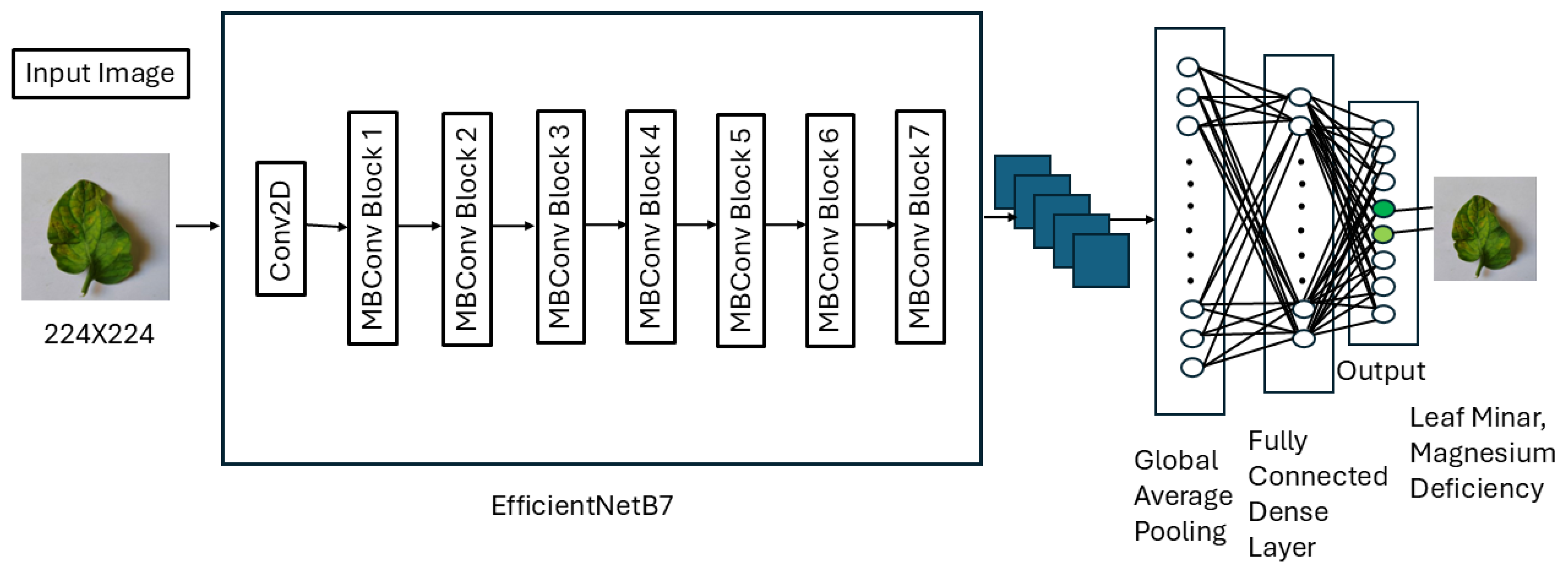
The EfficientNetB7 model was pretrained on the ImageNet dataset and was optimized for multi-label plant disease classification in this study. The EfficientNetB7 architecture was chosen for its exceptional performance in image recognition tasks and computational efficiency. ImageNet, which contains millions of images spanning thousands of classes, provided a robust foundation for feature extraction. To enhance the model’s accuracy, additional layers were integrated into the existing architecture. The overall design of the proposed model is illustrated in Figure 1.

During the initial training phase, the pretrained layers of EfficientNetB7 were frozen to function as a feature extractor. To reduce the spatial dimensions of the extracted features and minimize model complexity, a Global Average Pooling (GAP) layer was utilized. This layer also reduced the total number of parameters, improving computational efficiency, and mitigating the risk of overfitting. By avoiding dense and flattening layers immediately after convolutional layers, the model preserved critical features while maintaining simplicity. For regularization, a Dropout layer with a rate of 0.6 was employed. Through experimentation, this rate proved to be optimal, randomly deactivating 60% of activations during the forward pass in training. This reduced the model’s dependency on specific features, promoting generalization. A Dense layer with sigmoid activation was incorporated for multi-label classification, ensuring independent predictions for each disease label. The sigmoid function was selected over softmax because multi-label classification involves non-exclusive labels, whereas softmax is suited for mutually exclusive classes. The output layer was configured with nodes equal to the number of disease labels. The final model was constructed by integrating the custom layers with the pretrained EfficientNetB7 model. The input remained consistent with the base model, and predictions were generated through the added layers. The model was then compiled using the Adam optimizer, binary cross-entropy loss function, and accuracy as the evaluation metric. Adam was chosen for its adaptability and superior performance compared to alternatives such as Adamax, SGD, and AdamW. Its combination of the benefits of AdaGrad and RMSProp made it particularly suitable for this task. Binary cross-entropy was used as the loss function because it treats each label as a separate binary classification problem, fitting the requirements of multi-label classification. We calculated accurracy using the following equation:

$$\mathrm{Accuracy}={\displaystyle \frac{1}{N\times C}}\sum _{i=1}^N\sum _{j=1}^C\mathbf{1}(\sigma ({\widehat{y}}_{ij})>0.5=y_{ij})$$

(1)

where the number of samples is denoted by N, the total number of labels by C, the ground truth for the j-th label of the i-th sample is denoted by $y_{ij}$, and the anticipated probability following the application of the sigmoid activation function is denoted by $\sigma ({\widehat{y}}_{ij})$.

While accuracy was the primary metric for model performance evaluation, additional metrics such as precision, recall, and F1 score were later calculated to provide a comprehensive assessment. Moreover, model summary was generated to confirm the architecture, layer types, and parameter counts. This step ensures that the model’s structure aligned with the problem’s requirements, validating that the number of parameters is appropriate for efficient training and inference.

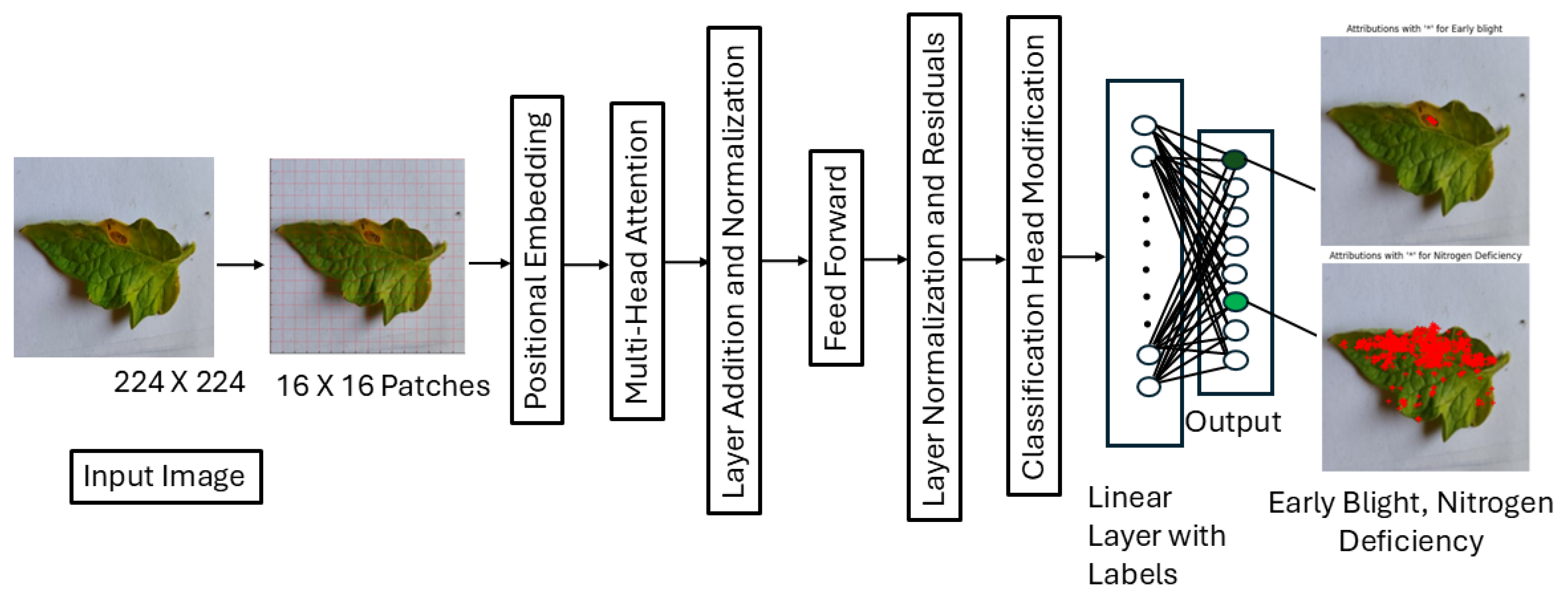
Figure 2 depicts the architecture of the ViT model. In order to manage data loading, a unique dataset class called ImageDataset was created. This class preprocessed photos using the Hugging Face ViTImageProcessor for tokenization and TensorFlow’s Keras tools for resizing. For compatibility, the labels are transformed into tensors. By adjusting the number of output labels and designating the disease type as multi-label classification, the model makes use of the ViT-Base (vit-base-patch16-224-in21k) model, which is pretrained on ImageNet-21k and consists of 12 transformer layers with 768 hidden units, 12 attention heads, a patch size of 16 × 16, an input resolution of 224 × 224, a feedforward dimension of 3072. To deal with multi-label output, a binary cross-entropy loss function with logits (BCEWithLogitsLoss) is used.

3.4. Training and Optimization

For the purpose of this study, we used images with a resolution of 224 × 224 and a batch size of 32. After experimenting with various batch sizes and epoch numbers to optimize accuracy, we settled on a batch size of 32 and 100 epochs based on the results. The dataset was divided into 80% for training and 20% for testing and validation. While the training generator provided shuffled and augmented data to enhance generalization, the validation generator supplied unshuffled data to accurately evaluate performance. To ensure optimal performance during training, we carefully monitored the process and adjusted parameters such as the learning rate to prevent overfitting. As we conducted training on the Google Colab platform, we utilized a model checkpoint mechanism to save only the best-performing version of the model based on validation performance. Additionally, learning rate scheduling was applied using the ReduceLROnPlateau callback. This technique reduced the learning rate when the validation loss plateaued for a specified number of epochs, enabling the model to converge more effectively by escaping local minima. Specifically, if no improvement was observed in the validation loss after five consecutive epochs, the learning rate was halved (factor = 0.5). The current learning rate was tracked in the training history, providing insight into its progression during training.

To prevent the learning rate from becoming excessively small, we set a minimum threshold of 1 × ${10}^{-6}$. This safeguard avoided scenarios where a very small learning rate could lead to prolonged training times, underfitting, or ineffective learning. Early stopping was also implemented to terminate training when validation performance ceased to improve, thereby mitigating overfitting. If no improvement in validation loss was observed for ten consecutive epochs, training stopped, and the model reverted to the weights of the epoch with the best validation performance.

Using the ReduceLROnPlateau scheduler based on validation loss, the training loop of our ViT model dynamically modifies the learning rate at the same time optimizing the model with the AdamW optimizer. So we decided to continue with the AdamW optimizer. Binary cross-entropy on logits was used to train the model, considering each label separately. We employed a sigmoid activation and a global threshold of 0.5 for reporting accuracy in order to convert predicted probability to binary labels. During preliminary tuning, this threshold was selected because it yielded the best overall balanced accuracy on the hold-out validation set. The model computes the loss, backpropagates gradients, changes weights, and then makes predictions using a forward pass during training. Loss, accuracy, and the best-performing epoch are among the parameters that are assessed and recorded by the training and validation loops like other models. After each epoch, the learning rate was also recorded to track its development.

After training, we applied Explainable AI (XAI) techniques, including Grad-CAM, Integrated Gradients, and LIME, to enhance interpretability. These methods highlighted the image regions most influential in the model’s classification decisions, providing valuable insights into its decision-making process. This not only improved trust in the model, but also offered a clearer understanding of its behavior, making it more transparent and reliable for practical applications.

3.5. Implementation of XAI to Enhance Model’s Interpretation

3.5.1. Integrated Gradient Implementation

A deeper comprehension of the developed neural model’s decision-making process is made possible by Integrated Gradients (IG), which provides a methodical way to determine how each unique input characteristic contributes to the model’s predictions. While implementing IG, we followed the steps discussed below:

• Creation of Baseline: To fit the desired input size of the model, the input photos were shrunk. The pixel values were adjusted to fall between 0 and 1. We used a Gaussian-blurred version of the original image to establish a baseline image for IG computation. By acting as a reference point, this blurring baseline ensures that the calculated gradients emphasize significant deviations from a “neutral” input condition. Since deep learning models frequently require floating point values, the input picture and baseline are transformed to the float data type to guarantee that the model and gradients computations may be completed accurately in floating point format.

  −

  Interpolation: Between the input image and the baseline, a number of interpolated images were produced. In order to provide a continuum of inputs for gradient computation, this was accomplished by linearly interpolating pixel values across several steps. Different amounts of “information” are represented by these interpolated images, which range from complete information (the input image) to no information (the baseline). The function creates steps + 1 images between the baseline and the input image for the steps number (by default, 50). As the image progressively moves from the baseline to the input image, this interpolation aids in understanding how the model’s forecast changes.

  −

  Calculate Gradient: For each interpolated image, gradients with the expected probability for the target label were calculated using TensorFlow’s “GradientTape”. For some reason if the baseline is not present there, our model performed blurring or used a black image itself. We used “GradientTape” for automatic differentiation so that we can use it further. Here a dictionary was created that contains the model’s output for every interpolated image. The model’s prediction for the target class for every interpolated image is then represented by a variable named “target_predictions”, which are subsequently extracted. The gradients of the model’s predictions in relation to the interpolated images are calculated by the “tape.gradient” function. This illustrates how responsive the model’s output is to modifications made to the input picture.

  −

  Combining Gradients: Gradients were multiplied by the difference between the input image and the baseline after being averaged over the interpolation stages. The average gradient across all interpolated images is obtained after the gradients have been calculated. Scaling the averaged gradients with the difference between the input image and the baseline yields the final Integrated Gradients attribution, which is then delivered as a NumPy array. This resulted in an attribution map that showed how crucial each pixel was to the model’s prediction.

• Visualization of Attribution: To visualize the output, attributions were calculated by summing the positive contributions of all the color channels. This process generated a multidimensional attributions array that represented how each pixel or feature influenced the model’s predictions. Contributions across color channels were reduced to a single channel using np.sum(attributions, axis=-1). Negative values were removed using np.maximum(attribution_mask, 0) to focus solely on positive contributions, highlighting the features that increased the model’s confidence in its predictions.
  For better visualization, the resulting attribution map was normalized to scale the data between 0 and 1. The normalized map was then converted to a heatmap using the JET colormap, applied with the cv2.applyColorMap function. This heatmap used a gradient of colors from blue to red to represent low to high attributions, providing a clear visual representation of the model’s focus areas.
  To further enhance interpretability, dilation and blending techniques were applied. The cv2.dilate function emphasized high-attribution regions by expanding them, while the cv2.addWeighted function blended the heatmap with the original image. This overlay allowed for an intuitive and easily interpretable visualization, highlighting the areas of the image that contributed most significantly to the model’s output.
• Original Image with Overlaying Heatmap: After successful completion of the process of baseline creation, heatmap creation, and other calculations we performed the visualization of the overlying heatmap on the original image. In order to do that, we took an image and rescaled it to [0, 255] using img[0] * 255 after being normally adjusted to the range [0, 1]. For OpenCV compatibility, the heatmap, which is likewise in the [0, 1] range, is scaled to [0, 255].
  The original image and the heatmap are combined using the “cv2.addWeighted” function, so that 60% of the original image and 40% of the heatmap are shown. This makes the heatmap semi-transparent while preserving the image features. “Plt.imshow()” is used to display the blended result. The image is finally rendered with the attribution heatmap superimposed for interpretation using “plt.show ()”.

3.5.2. Grad-Cam Implementation

• Configuration of Grad-CAM: Grad-CAM was configured to identify significant regions in an image by associating the gradients of the target class’s output with the activations of the final convolutional layer, “top-conv.” A submodel was developed to output both the final prediction probabilities and the activations of the “top-conv” layer. This design ensured that Grad-CAM could link specific predictions with the corresponding activation maps. During a forward pass, this sub-model processed the input plant image to produce both the model’s prediction and the activation maps.
• Gradient Calculation: Gradients for the target plant disease label’s predicted probability were calculated relative to the activations of the “top-conv” layer using TensorFlow’s GradientTape. These gradients were averaged spatially (pooled) to create channel-wise significance weights, reflecting the importance of each feature map. If no target label was explicitly defined, the system automatically selected the label with the highest predicted probability for analysis.
• Heatmap Generation:

  −

  A vector representing the significance of each feature map was created by pooling the gradients across spatial dimensions. The feature maps were then weighted by these pooled gradients, generating a weighted sum to produce the Grad-CAM heatmap. The resulting heatmap highlighted the areas most influential for the target prediction. Values were normalized to a range of 0 to 1, and negative values were clipped to zero, simplifying the interpretation of important regions.

  −

  The normalized heatmap was returned as a NumPy array and overlaid onto the original image for visualization. This overlay provided an intuitive understanding of the model’s focus areas, with higher heatmap values corresponding to regions most critical to the prediction.

  −

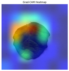
  The heatmap was rescaled from [0, 1] to [0, 255] in order to adhere the image formats after the image has been loaded and transformed into a NumPy array. After applying a ’jet’ colormap, which uses color assignment to indicate pixel importance, the heatmap is scaled to fit the original image’s proportions. The transparency of the heatmap was then changed by superimposing it on the original image using a weighted sum that is managed by the alpha parameter. Matplotlib is used to display the combined image, allowing users to see the regions of the image that the model concentrated on. The Grad-CAM heatmap, which offers insight into the model’s decision-making process, is created and shown after the image has been preprocessed for the model.

3.5.3. LIME Implementation

LIME stands for Local Interpretable Model-agnostic Explanations. LIME provided us with a transparent model that helped us to understand how multi-label disease predictions are made. LIME identifies the crucial regions of a plant leaf that assist in the prediction of one or more diseases by decomposing the model’s intricate decision-making process into easily understandable parts.

• Lime Preprocessing:

  −

  Input to LIME: To make sure that every image satisfies the input specifications of the deep learning model being used, the first step in preparing the data for LIME is to resize the images to a constant size, usually defined as IMG_SIZE × IMG_SIZE. The model can analyze the photos in a uniform way thanks to this resizing, which guarantees consistency. Furthermore, the photos’ pixel values are adjusted to the range [0, 1]. In order to normalize the input data and make it more consistent with the circumstances in which the model was trained, this normalization phase is essential. Again, normalization guarantees that the learning process is not dominated by any particular pixel value. In order to make it easier to generate explanations using LIME, each image is finally transformed into a format appropriate for additional analysis, including segmentation.

  −

  Segmentation: A crucial stage in the LIME implementation is segmentation, which divides the image into meaningful areas called superpixels. LIME can more easily determine which areas of the image have the greatest influence on the model’s predictions when it uses superpixels, which are contiguous patches of pixels grouped according to color and texture similarity. The Quickshift algorithm was used to carry out this segmentation. Pixels are clustered using the Quickshift technique to optimize similarity while taking spatial closeness into account. A kernel size of three, which established the size of the filtering zone, and a maximum distance (max_dist) of six, which restricts the separation between pixels within a single superpixel, are important parameters for this segmentation.

• Lime Explanation:

  −

  Samples that have been perturbed: LIME (Local Interpretable Model-agnostic Explanations) begins with creating images that have been perturbed. This is accomplished by hiding or masking specific superpixels in the picture. Every perturbed image is a minor modification of the original, with some areas (superpixels) covered or eliminated. To evaluate how these changes in certain locations affect the model’s output, the predictions made by the model are documented for each perturbed version. LIME learns the importance of each region in influencing the model’s decision-making process by examining how the predictions of the model alter when various superpixels are hidden.

  −

  Model Surrogate: LIME trains a local surrogate model, usually a straightforward linear regression model, using predictions from the modified images. Within the immediate neighborhood of the input image, this surrogate model closely resembles the behavior of the original, more sophisticated model. The influence of specific features in our model, the superpixels, may be better understood thanks to the surrogate model’s simplicity and interpretability. The surrogate model’s coefficients showed how important each superpixel was, giving information about which areas of the image are most crucial for the model’s predictions. These coefficients made it easier for us to understand how certain areas of the image impact the result by providing a clear and understandable explanation of the model’s behavior.

• Visualization: LIME creates two different representations for every disease label when the model’s confidence surpasses a predetermined threshold after the surrogate model has been trained and the significance of each superpixel has been established. In the proposed model, the threshold of 0.5 produced the best outcome.

  −

  Masked Explanation: Only the most important superpixels that positively impact the predicted outcome of a certain disease are highlighted in this depiction. According to the model, these areas have the most impact on the result. The masked explanation provides useful information about the aspects the model deems critical, helping to identify the precise areas of the image that are most crucial to the prediction.

  −

  Superimposed Image Explanation: The original plant image is overlaid with the highlighted superpixels from the masked explanation. By combining the original image with the regions that were most crucial to the model’s prediction, a visual summary is produced. The superimposed explanation enables users to directly observe which sections of the image are being evaluated as suggestive of disease by visibly overlaying these crucial locations.

4. Result and Discussion

4.1. Training and Validation Results

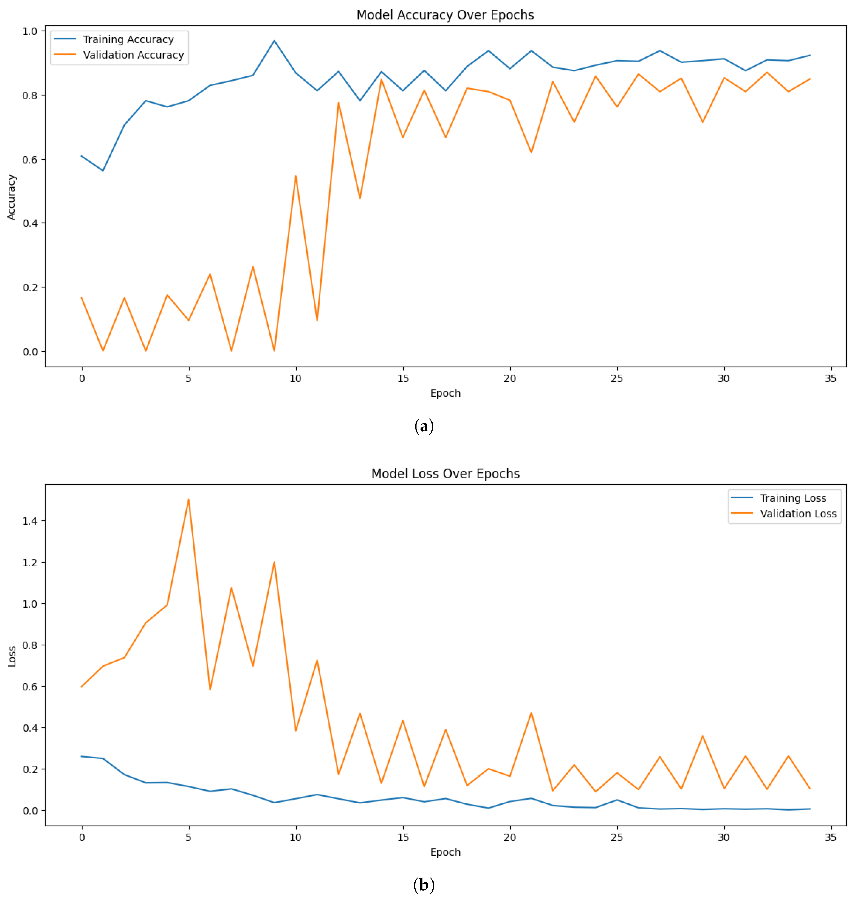
In the multi-label classification test for identification of tomato leaf diseases, the proposed approach yielded promising results. The models effectively learned the patterns and characteristics associated with multiple diseases present on tomato leaves. Among the models, EfficientNetB7 demonstrated strong performance, achieving a maximum training accuracy of 96.88%, and validation accuracy of 86.98%. The validation loss of 0.0907 further highlights the model’s ability to generalize well to unseen data. 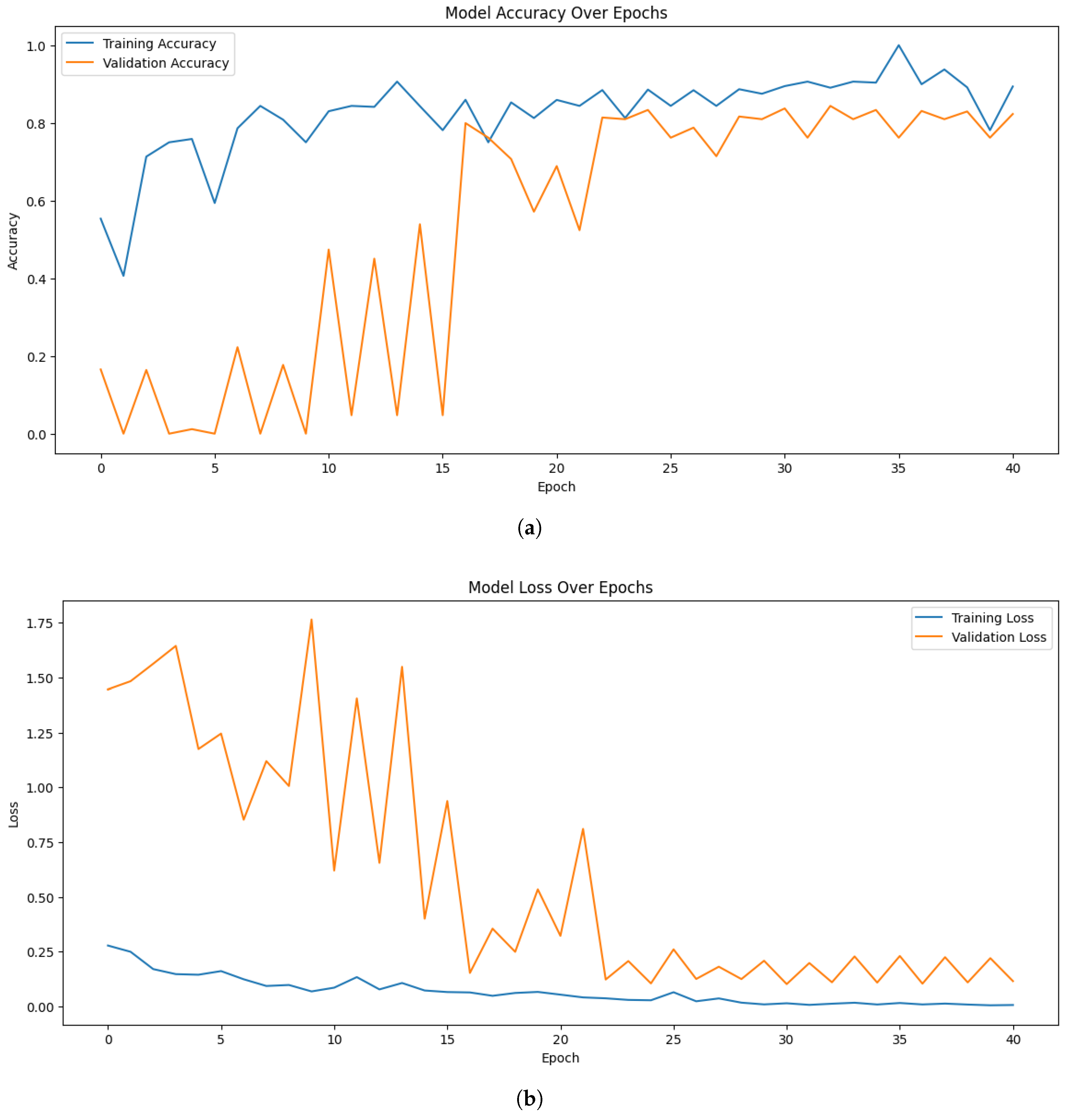Figure 3 illustrates the accuracy and loss trends for the proposed EfficientNetB7 model. Similarly, when experimenting with EfficientNetB0, the highest training, and validation accuracy were 93.75%, and 82.00% respectively. In comparison, ResNet50 achieved a maximum training accuracy of 87.50%. Figure 4 presents the accuracy and loss curves for the proposed EfficientNetB0 model.

Although EfficientNetB0 and EfficientNetB7 performed well, there were some fluctuations in their validation accuracy curves over different epochs. The class imbalance and the small size of the dataset are partially attributed to this, as they may have an impact on the model’s ability to generalize. Additionally, although generally advantageous, the diversity brought about by data augmentation might have occasionally caused differences in validation behavior. The overall patterns show steady convergence and strong generalizability despite these oscillations.

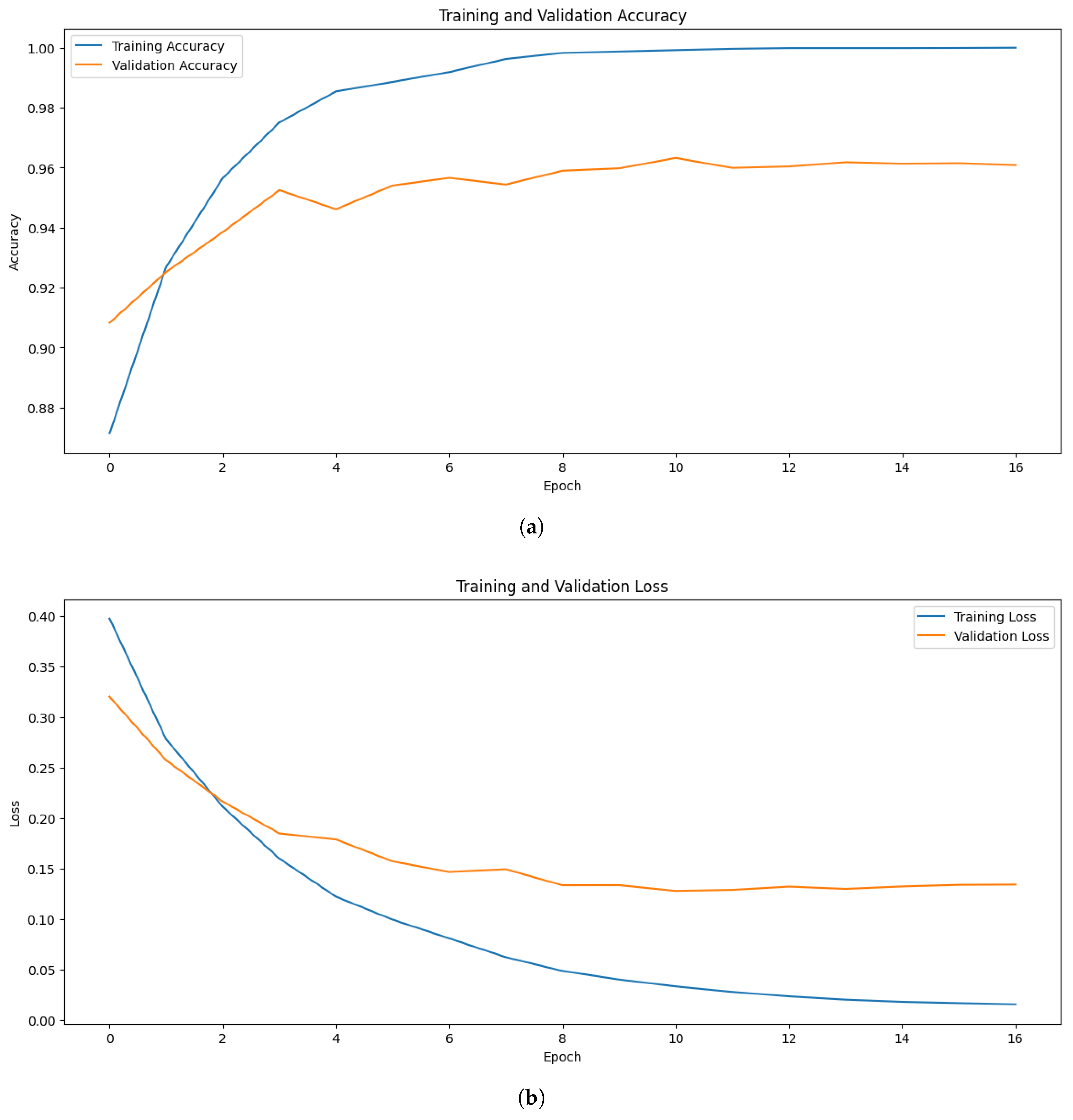
Building upon these results, the Vision Transformer (ViT) model pushed the accuracy even further, achieving a perfect 100.0% training accuracy, with an impressive validation accuracy of 96.39%. This substantial improvement highlights the effectiveness of transformer-based architectures in capturing complex patterns in multi-label classification tasks. Figure 5 visualizes the accuracy and loss of the ViT model.

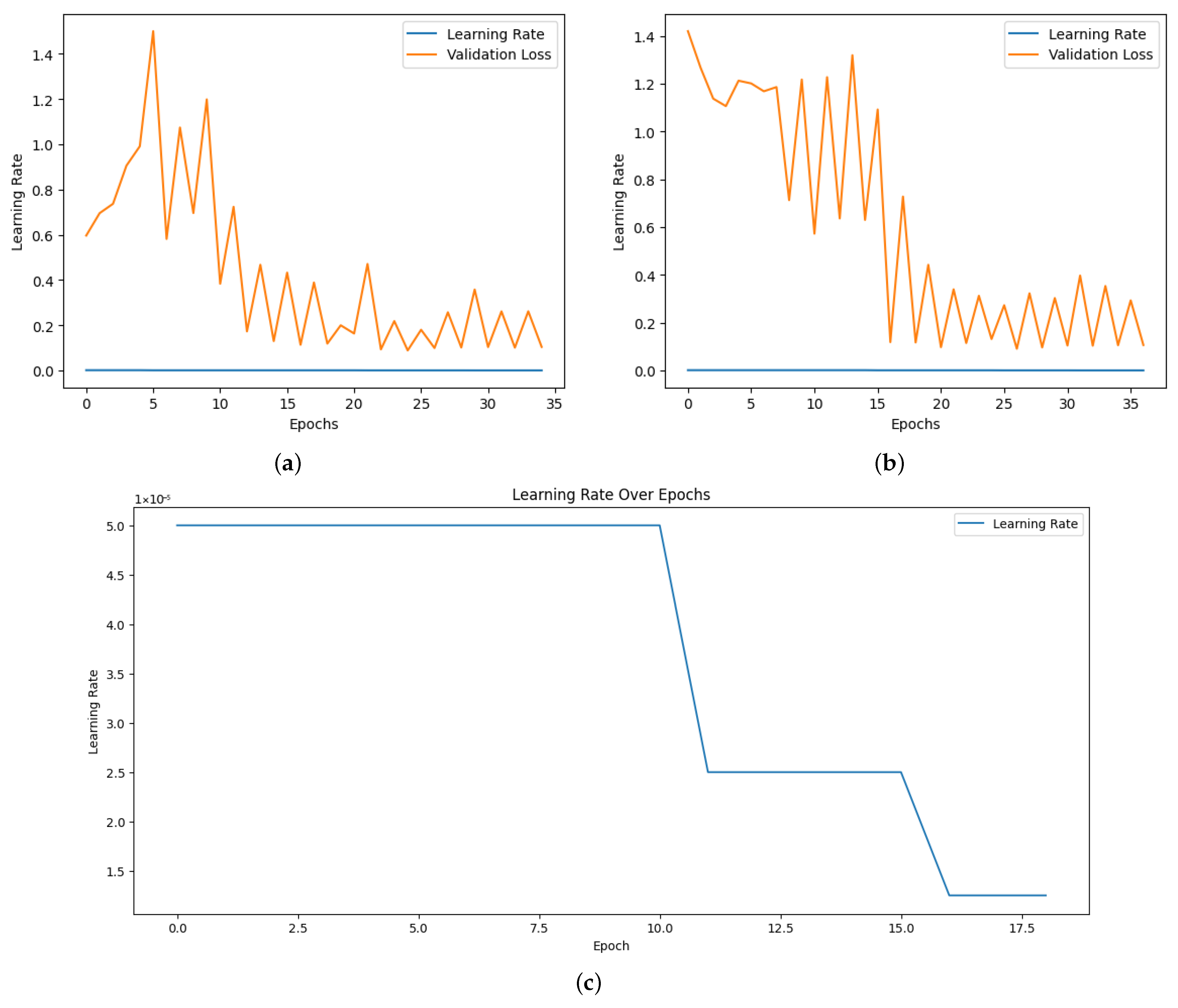
The model’s performance was greatly improved by optimization techniques, such as early stopping and learning rate scheduling. By dynamically modifying the learning rate during training, “ReduceLROnPlateau” allowed the model to converge effectively without experiencing overfitting or local minima. To preserve the optimal weights for assessment, early stopping was implemented as soon as the validation performance plateaued. The efficacy of these optimization strategies was further supported by the observation that the validation loss continuously decreased during the training phase, which corresponds with the steady improvement in testing and validation accuracy. Figure 6 shows the learning rate adjustment for the EfficientNetB7, EfficientNetB0 and Vi models.

In addition to optimization techniques such as early stopping and learning rate scheduling, we conducted an ablation study to evaluate the impact of key architectural and preprocessing components. The ablation results are summarized in

Table 2. Ablation study results for architectural and preprocessing variations.

Variant	Train Accuracy	Validation Accuracy	Validation Loss
Baseline	0.922132	0.907636	0.227652
A1—No Augmentation	0.945699	0.903834	0.254597
A2—No Dropout	0.931757	0.912706	0.217861
A3—Patch Size 8	0.929895	0.905577	0.220887
A4—Patch Size 32	0.925935	0.905735	0.227383
A5—No Rescaling	0.911122	0.889575	0.253319
A6—Fewer Layers	0.930212	0.902883	0.234469

and demonstrate how changes such as removing data augmentation or modifying patch sizes influence both training and validation accuracies.

4.2. Model Testing Performance

In contrast to Gehlot et al. [16], which evaluated performance solely based on training accuracy, our approach provides a comprehensive assessment of generalization by testing and evaluating the models on a newly unseen dataset using metrics such as F1 score, precision, recall, AUC, and ROC curves—demonstrating their robustness and reliability in real-world multi-label classification tasks.

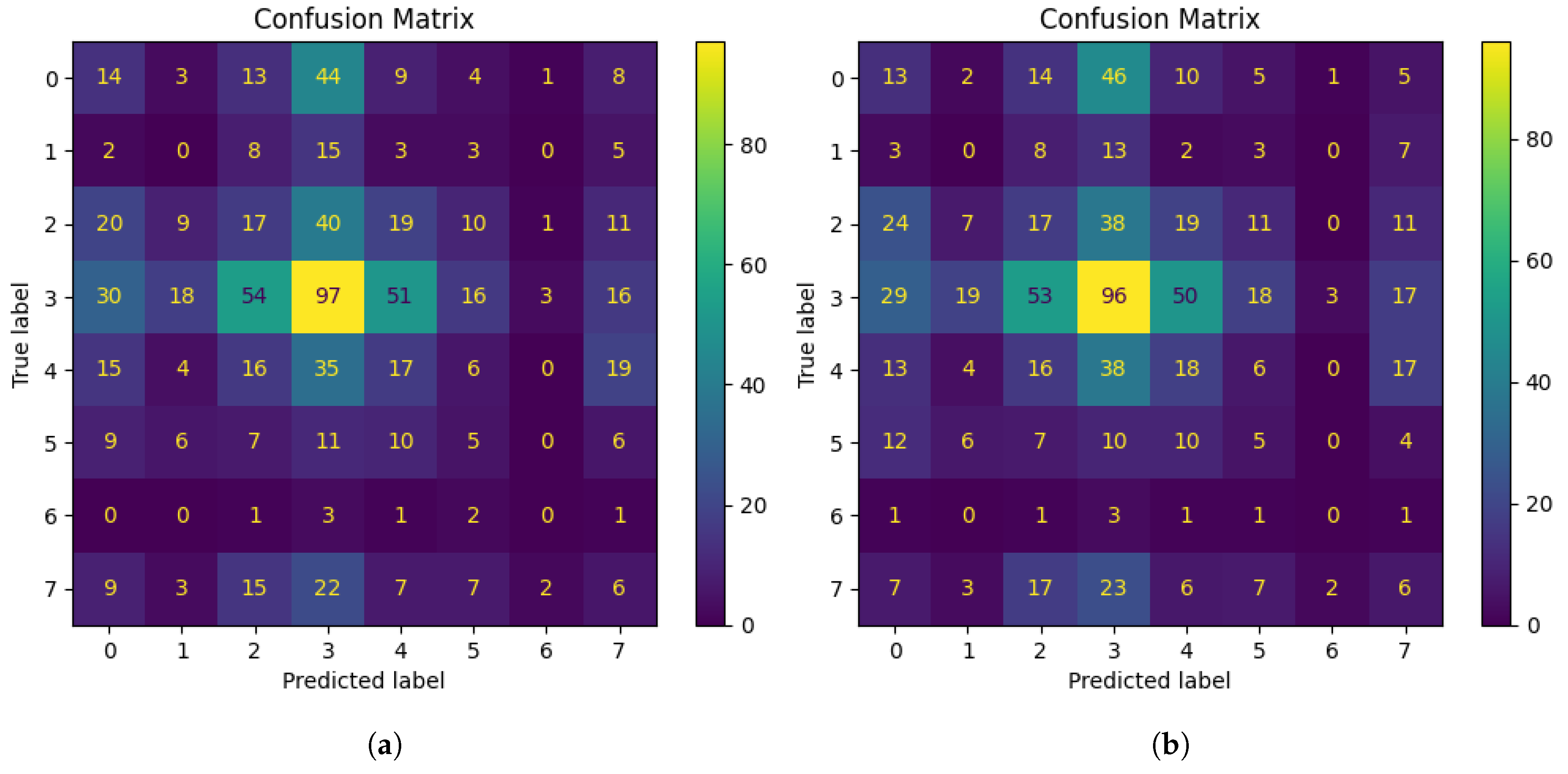
We achieved a test accuracy of 95.99%, 85.48%, and 81.95% from the Vi model, EfficientNetB7 and EfficientNetB0 respectively. To further assess class-wise performance, we analyzed the confusion matrices of EfficientNetB7, EfficientNetB0, and the ViT model. The matrices for the EfficientNets are provided in Figure 7. They show that disease class 4 was successfully identified by both EfficientNetB0 and EfficientNetB7. For this class, EfficientNetB0 achieved 96 correctly categorized cases, but EfficientNetB7 showed a little improvement in accuracy with 97 correctly classified instances. The fact that both models consistently perform well for disease class 4 indicates that they are both capable of recognizing diseases with unique characteristics and trends.

EfficientNetB0 frequently mistook disease class 0 with disease classes 2 (24 cases) and 3 (46 cases). With 20 and 44 misclassifications for classes 2 and 3, respectively, EfficientNetB7 demonstrated a modest improvement. In both models, they were incorrectly identified as disease classes 3 and 4, however, EfficientNetB7 slightly decreased these errors (from 23 to 22 for class 3 and from 7 to 6 for class 4). For disease classes 1 and 5, the models continuously performed worse than expected. There were 13 and 10 accurate classifications in EfficientNetB0, respectively. Slightly improved to 15 and 11 correct classifications, respectively, in EfficientNetB7. These classes might have small changes in their features that are more difficult for the models to detect.

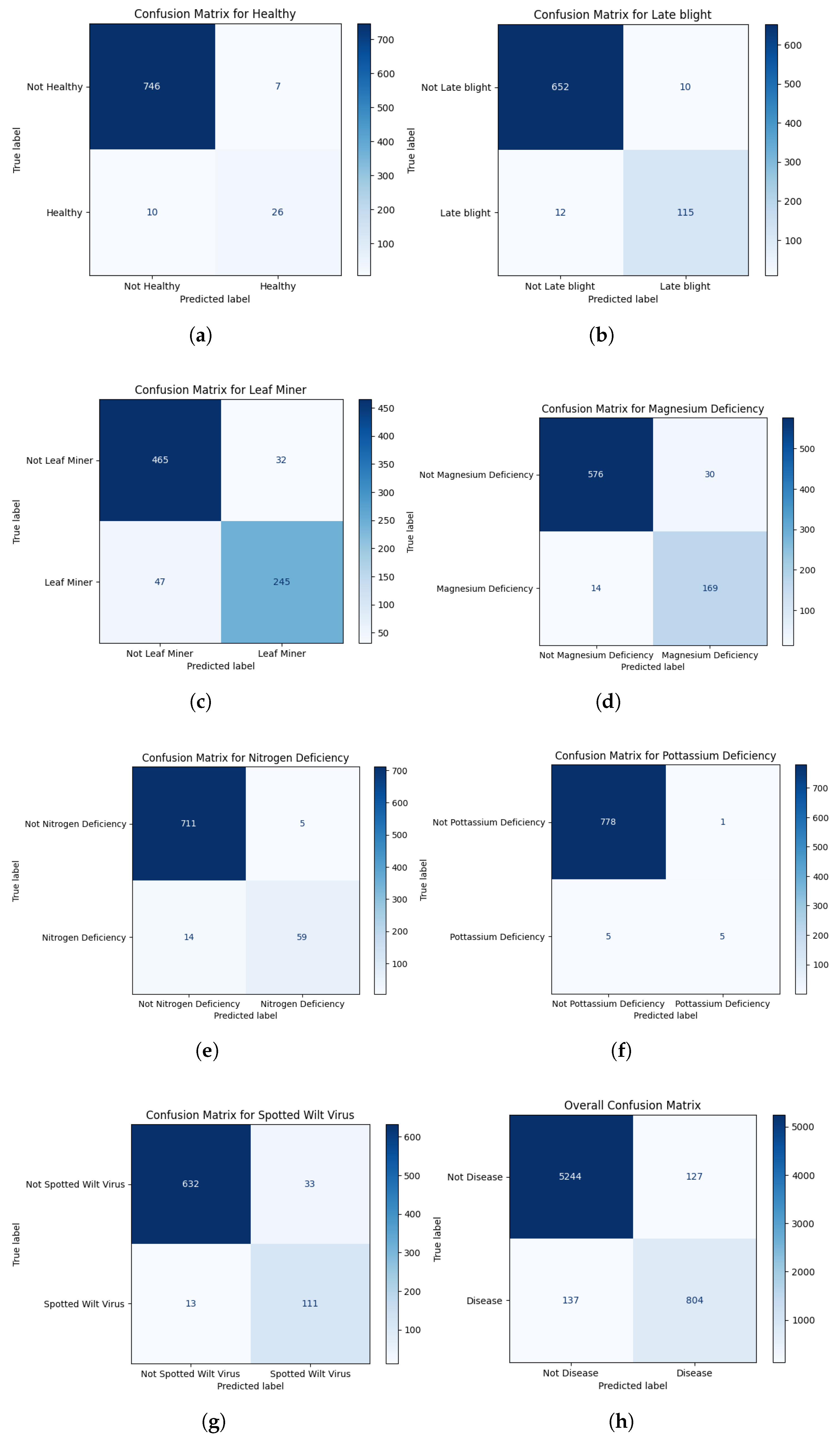
Figure 8 depicts the confusion matrices for different classes that we obtained from the Vi model. Each of the confusion matrices provides a transparent view of the performance of the model. In the classes where the EfficientNet models were struggling, the ViT model performed significantly better and showed considerable improvement.

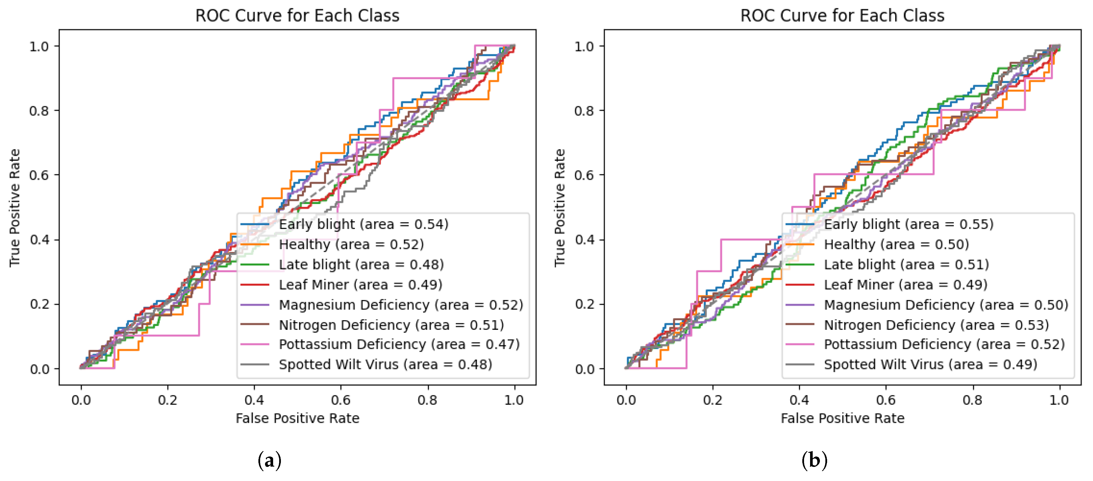
From Figure 9, we can see the Receiver Operating Characteristic (ROC) curves of both EfficientNet models. With minor improvements in the Area Under the Curve (AUC), EfficientNetB7 is more effective for predicting early blight and nitrogen deficiency. The AUC for potassium deficiency improved significantly from 0.47 to 0.52 in EfficientNetB7. And there was little to no improvement or a minor decline in classes such as leaf miner, magnesium deficiency, and healthy leaves. The marginal overall improvement in AUC values indicates that EfficientNetB7 outperforms EfficientNetB0 in terms of discriminative performance for specific classes, but not consistently.

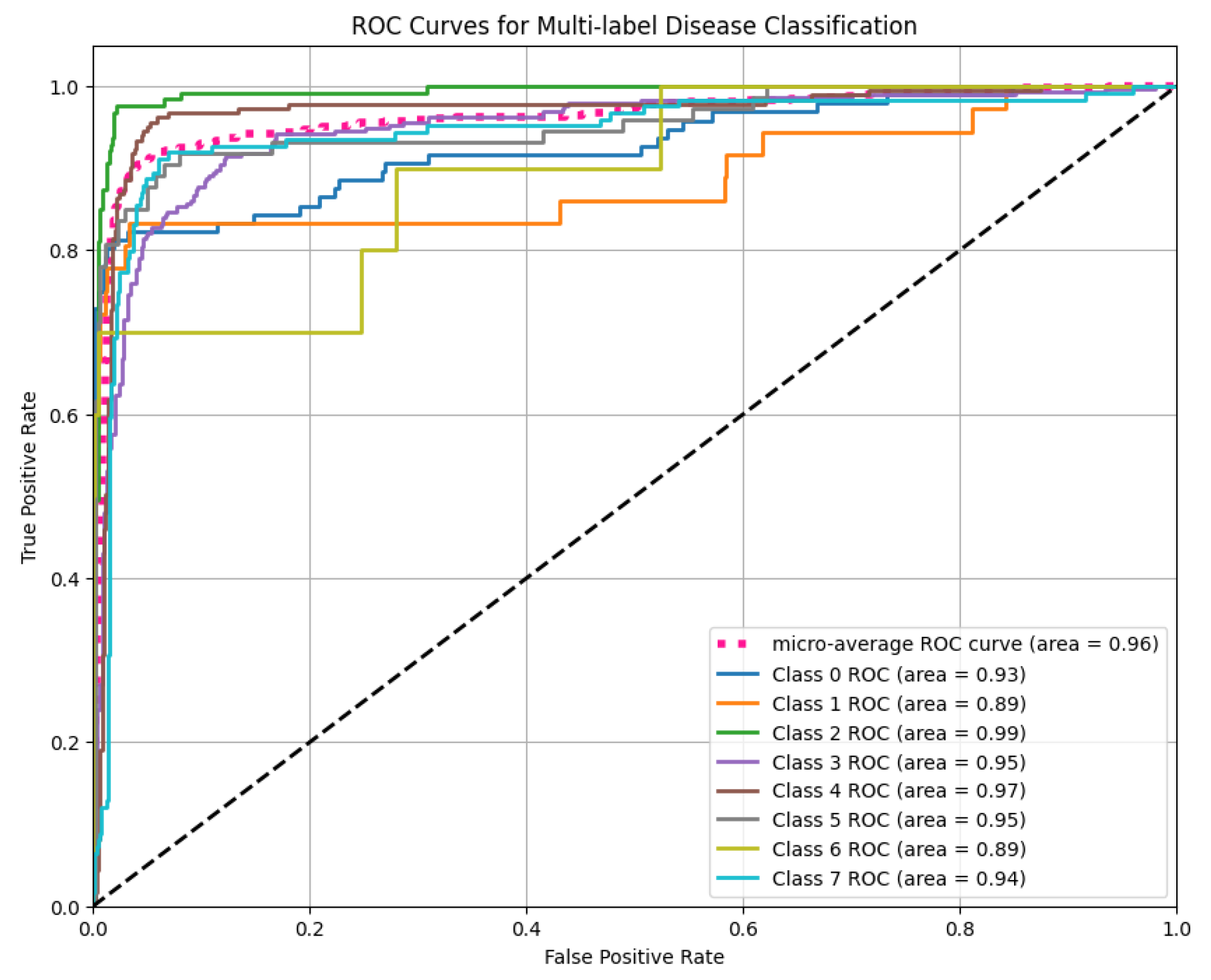
As these results suggest some class-wise variation but highlight the models’ limitations in consistent disease discrimination, to improve performance, we developed a Vision Transformer (ViT) model, which significantly outperformed both EfficientNet variants. To evaluate the ViT’s discriminative ability across all disease classes, we plotted the ROC curves for each label and computed the AUC. As illustrated in Figure 10, the ViT model achieved a micro-average AUC of 0.96 and a macro-average AUC of 0.94, reflecting its strong ability to generalize across multiple disease labels. The per-class AUC values also remained consistently high, ranging from 0.89 to 0.99, indicating reliable performance in distinguishing between various tomato leaf diseases.

The results from k-fold cross-validation and performance metrics for the EfficientNets highlight the challenges in generalization and classification capabilities. While training accuracy was relatively high across folds, validation accuracy remained consistently low, suggesting overfitting and potential class imbalance issues. Precision, recall, and F1 score analysis revealed further insights, with the “leaf miner” class achieving the highest F1 score of 0.38, indicating difficulties in distinguishing between these categories. This disparity likely stems from class imbalance or insufficient learning for underrepresented classes.

The model’s micro-averaged precision (0.22) and recall (0.22) further emphasize its struggles with generalization, potentially due to suboptimal thresholding for multi-label predictions. To address these issues, strategies such as applying regularization techniques, optimizing per-class thresholds, and addressing class imbalance through techniques like class weighting or oversampling should be explored. These improvements will be critical for enhancing the model’s ability to generalize and perform reliably across all classes.

This scenario was considerably improved in the Vi model with much better performance. With a training accuracy of 100.0%, a validation accuracy of 96.39% and a testing accuracy of 95.99%, the ViT-based multi-label disease classification model performs admirably, demonstrating that it has mastered the patterns in the training data and can effectively generalize to new data. We also obtained a recall of 0.87, F1 score of 0.86, and precision of 0.87, which indicates a sharp improvement in accurately recognizing all disease classifications. The model struggles to balance false positives and false negatives, as evidenced by the minor decline in F1 score when compared to precision and recall.

4.3. External Dataset Evaluation

In order to confirm the generalization capacity, we assessed our proposed models on another publicly accessible dataset named “Plant Pathology 2021 - FGVC8” [38]. To evaluate the model on this external dataset, 15% of the total images were allocated for testing. For this external dataset, the ViT, EfficientNetB7, and EfficientNetB0 models performed similarly, retaining good accuracy and F1-scores across all disease categories. In particular, the ViT model achieved training, validation, and testing accuracies of 100%, 96.9%, and 96.40% while the EfficientNetB7 model achieved training and validation accuracies of 96% and 85.84%, respectively. These findings clearly show that the suggested method is not overfitted to a particular data distribution and generalizes well beyond the Tomato-Village dataset, supporting its robustness and dependability. Furthermore, we performed an ablation study on the external dataset as shown in

Table 3. Ablation study results on the external dataset.

Variant	Train Accuracy	Validation Accuracy	Validation Loss
Baseline	0.9832	0.9652	0.0949
A1—No Augmentation	0.9834	0.9663	0.1010
A2—No Dropout	0.9868	0.9662	0.0915

.

4.4. Explainable AI Analysis

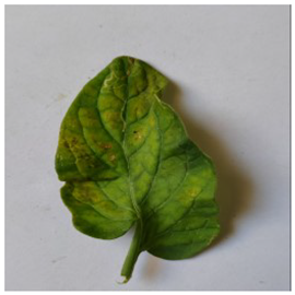
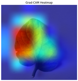
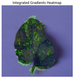
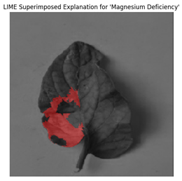
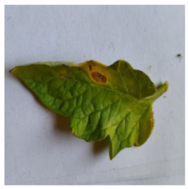
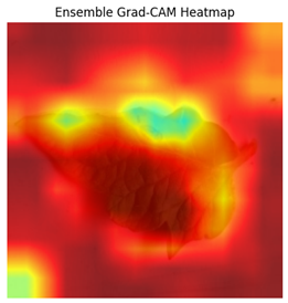
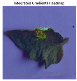
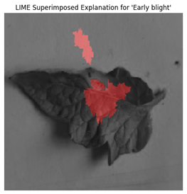
We used LIME, Grad-CAM, and Integrated Gradients to enhance transparency and interpret the model’s predictions. These methods offered intellectual and visual justifications for the model’s decision-making procedures as shown in

Table 4. Original Image with Outputs from LIME, Grad-CAM, and Integrated Gradients.

Leaves	Grad-CAM	IG	LIME	Disease
				Spotted wilt Virus✓
				Early blight virus✓ Potassium deficiency ✗
				Leaf miner✓ Magnesium deficiency✓
				Early blight✓ Leaf miner✓ Magnesium deficiency✓
				Early blight✓ Nitrogen deficiency✓

.

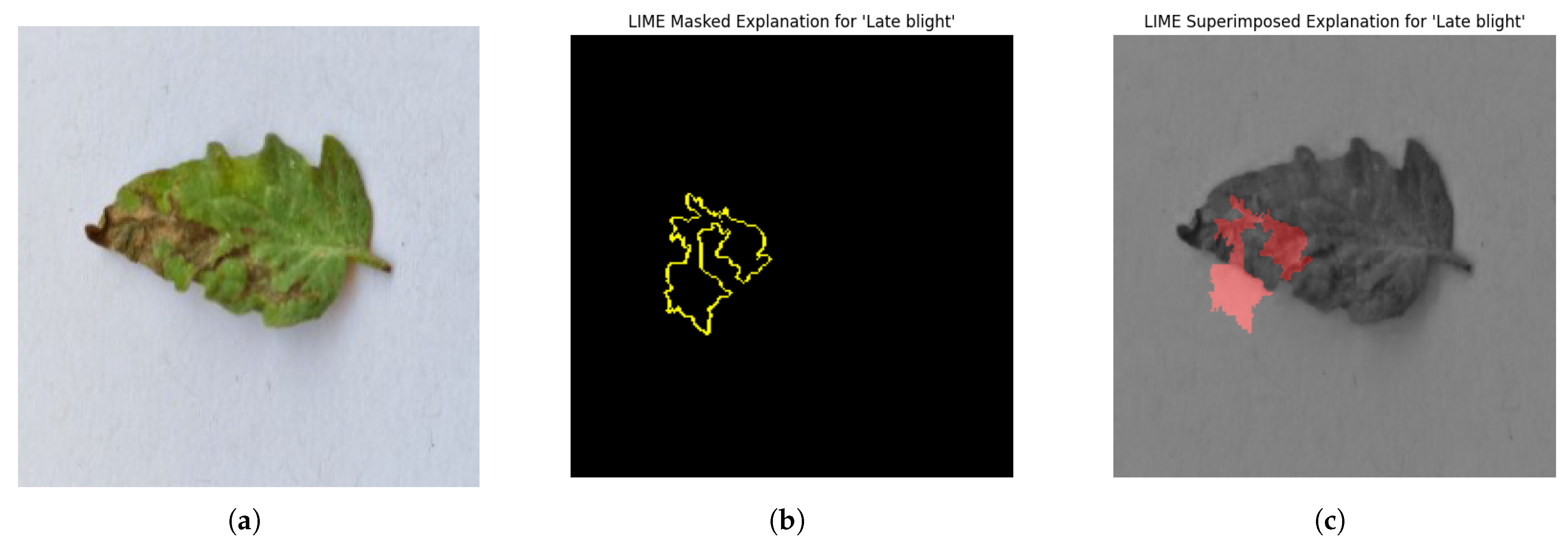
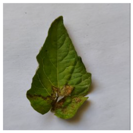
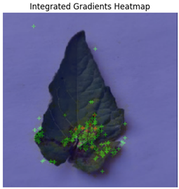
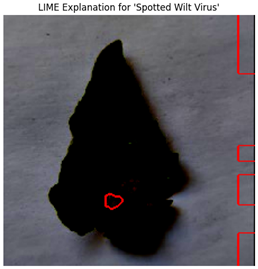
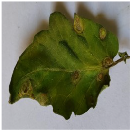
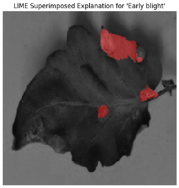
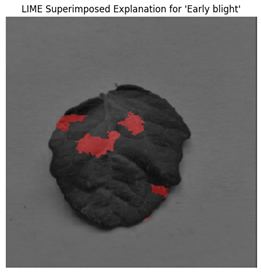
For each class prediction, LIME superimposed explanations emphasized particular areas of the input image that had the most influence. By effectively identifying regions pertinent to a certain disease class, LIME offered a clear insight into the model’s decision-making procedure. Sometimes, particularly in images with overlapping or subtle elements, the superimposed explanations included noisy areas that we can see in Figure 11.

LIME seemed to be relatively less effective on the proposed model compared to the other two explainable AI techniques.

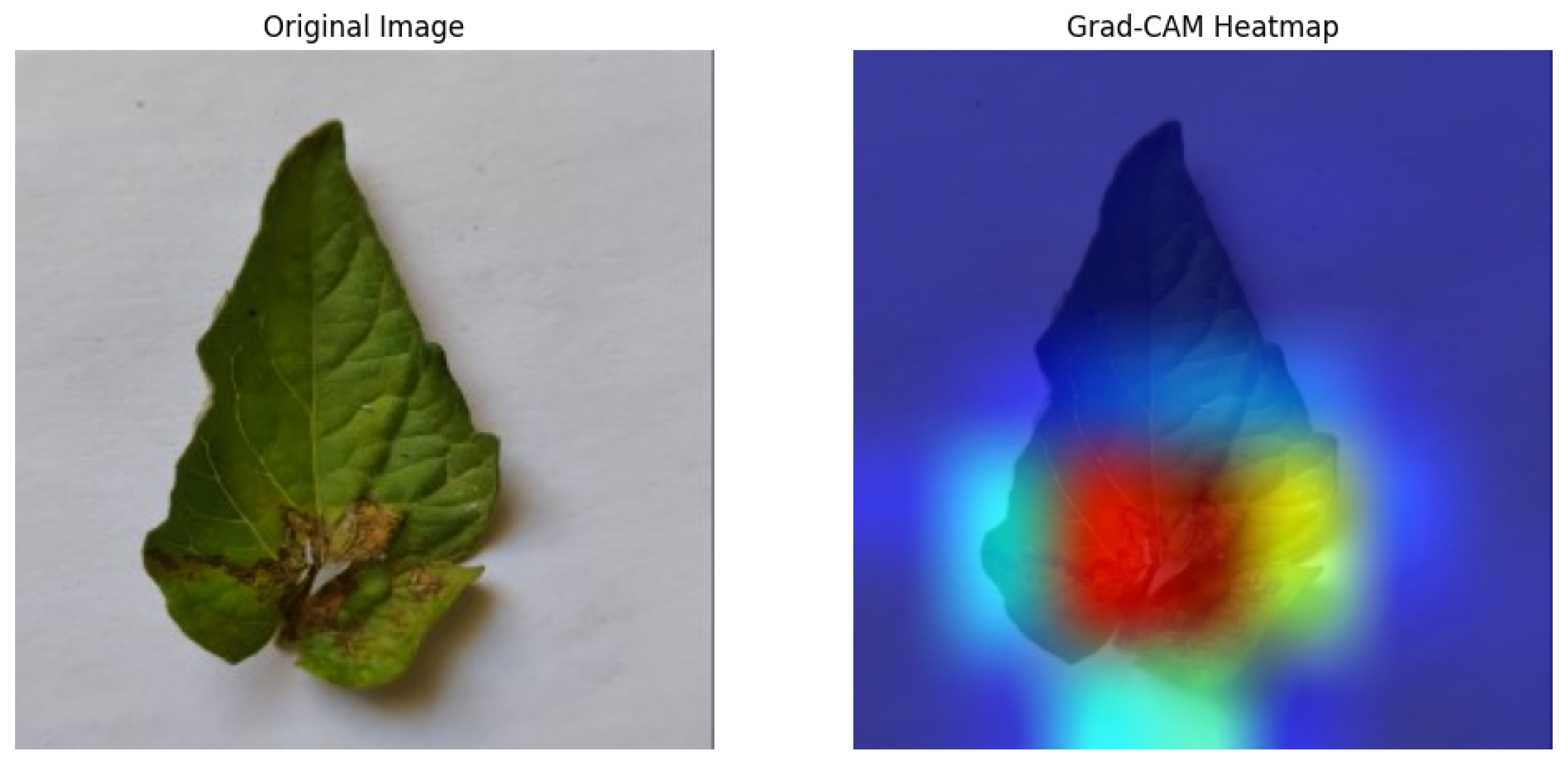
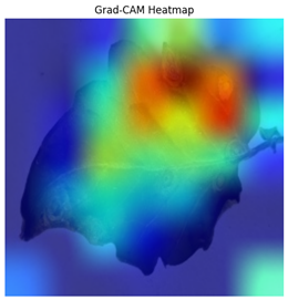
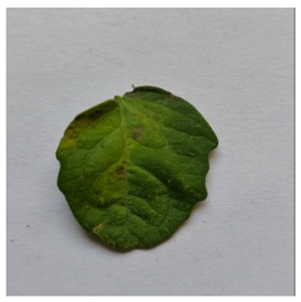
The Grad-CAM heatmap successfully showed symptomatic regions in Figure 12 for spotted wilt virus. But Grad-CAM occasionally had trouble separating features unique to a single disease in multi-label circumstances, which resulted in diffused heatmap patches. The Grad-CAM heatmap occasionally concentrated on irrelevant regions for diseases with faint visual signals (for example in Table 4), suggesting that the model’s interpretability can be further improved.

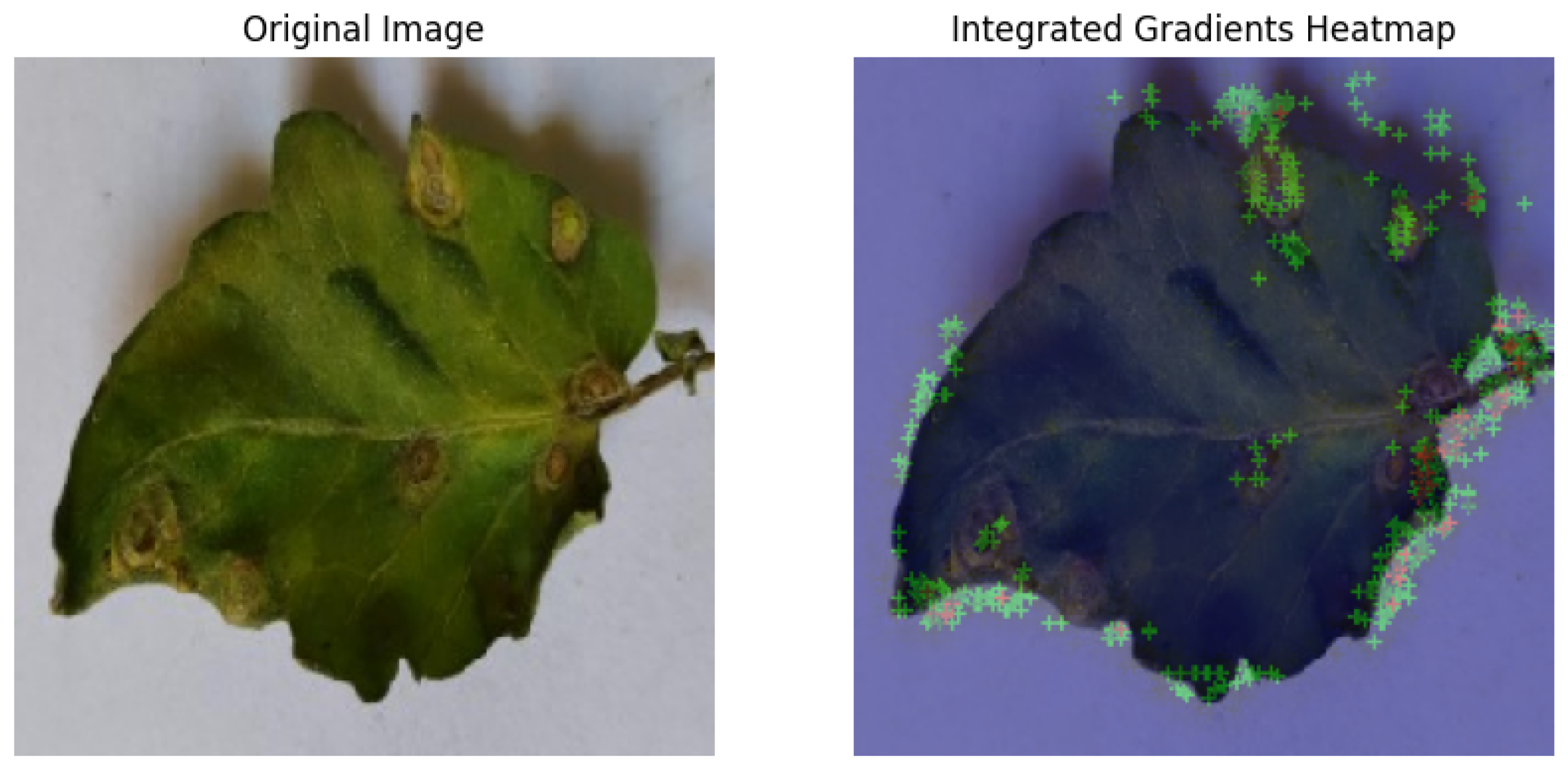
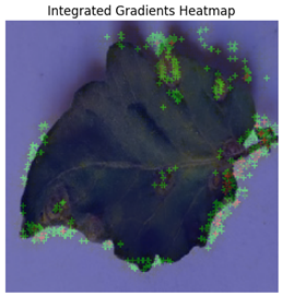
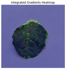
In Integrated Gradients, pixel-level attributions were provided, which showed which input pixels were most important in the model’s predictions. Figure 13 shows how Integrated Gradients identifies specific channels and their values.

This technique was especially helpful for identifying multiple disease spots depicted in Figure 14, because it highlighted discrete leaf sections that were consistent with apparent disease signs. Integrated Gradients displayed a more diffused pattern for diseases with less localized symptoms, indicating that the model may rely on broad patterns rather than particular markers. Integrated Gradients delivered more precise information regarding subtle symptom markers, whereas Grad-CAM presented broader regions of interest. Integrated Gradients performed the best among the three implemented explainable AI techniques.

The overall results of our proposed method show significant advancements in the identification of multi-label plant diseases. The highest training accuracy achieved by our ViT model is 100.00%, surpassing the 91.4% reported by any model from Gehlot et al. [16]. The training accuracy of our EfficientNetB0-based model was 93.75%, which is higher than the 87.00% training accuracy of Gehlot et al.’s EfficientNetB0 implementation. Additionally, our model outperformed the 77.30% reported in their implementation with a training accuracy of 96.88% when utilizing EfficientNetB7. Similarly, using ResNet50, our method obtained a training accuracy of 87.50%, surpassing Gehlot et al.’s 85.00%. The robustness of our training method and optimization techniques is demonstrated by our Vi implementation, which stands out among all models with the highest training accuracy of 100.00%.

Table 5. Comparative Accuracy Analysis of the Proposed Model vs. Existing Models.

Accuracy	Proposed Model	Gehlot et al. [16]
Highest Training accuracy	100.00%	91.4%
Vi Training accuracy	100.00%	N/A
EfficientNetB7 Training accuracy	96.88%	77.30%
EfficientNetB0 Training accuracy	93.75%	87.00%
ResNet50 Training accuracy	87.50%	85.00%

below shows the accuracy comparison between the proposed model and the existing model.

In addition to improved accuracies, a deeper understanding of disease prediction is made possible by the incorporation of explainable AI approaches into our model. To visualize and analyze the model’s decision-making process, Grad-CAM, LIME, and Integrated Gradients were used. When it came to correctly identifying unhealthy areas of plant leaves, Integrated Gradients continuously performed better than the others, providing more accurate and lucid visuals. The utilization of EfficientNet’s scalable architecture, a successful data augmentation approach, and improved hyperparameters are some of the reasons for our model’s exceptional performance. These developments not only increase training accuracy but also demonstrate our model’s resilience and dependability in detecting several diseases at once, which is an essential prerequisite for practical agricultural applications.

5. Conclusions

In this study, we developed three robust multi-label classification models for tomato plant disease identification by leveraging the EfficientNetB7, EfficientNewB0, and Vision Transformer (ViT) architectures alongside explainable AI (XAI) techniques. The models achieved remarkable training accuracies of 96.88%, 93.75%, and 100.00%, respectively, significantly outperforming benchmarks set by Gehlot et al. [16] and demonstrating superior performance in handling the complexities of multi-label classification.

Unlike the prior study that focused only on training accuracy, our approach demonstrates strong generalization to unseen data through rigorous evaluation on a separate test set using F1 score, precision, recall, AUC, and ROC curves, highlighting the superior robustness and reliability of our multi-label classification models. Additionally, the validation and the testing results showed consistent performance, with the ViT model achieving a validation accuracy of 96.39%, a testing accuracy of 95.99%, and a macro-average AUC of 0.94, confirming its effectiveness in capturing complex disease patterns across multiple labels.

To enhance transparency and trust, we incorporated XAI techniques, including Grad-CAM, LIME, and Integrated Gradients. Among these, Integrated Gradients proved particularly impactful, offering precise visual explanations by identifying diseased regions on plant leaves. This level of interpretability, often absent in prior models, bridges the gap between model performance and transparency, providing actionable insights for practical agricultural applications.

The findings underscore the strong potential of combining state-of-the-art deep learning architectures with explainable AI to address real-world challenges in plant pathology. While our model achieved high validation accuracy and demonstrated the value of explainability, it also highlighted areas for future improvement, such as addressing class imbalance, optimizing thresholds for multi-label predictions, and improving generalization through enhanced regularization and data handling strategies.

Additionally, preliminary evaluation of an independent external dataset yielded promising results that indicate a high degree of generalization, though larger-scale testing will be needed to substantiate this robustness. Future research could build upon this study by leveraging larger and more diverse datasets, which would improve the model’s generalization and robustness across various plant diseases and environmental conditions. Implementing the system on cutting-edge devices such as mobile platforms could also enhance its practicality for real-world agricultural applications. Moreover, a promising direction involves exploring hybrid explainable AI (XAI) techniques—such as combining Grad-CAM, LIME, and Integrated Gradients—to enhance both the performance and interpretability of the model. These advancements could lead to more trustworthy and actionable insights for end users like farmers and agricultural experts.