Identification Method for Critical Transmission Sections in Power Systems Based on Grid Partitioning and Power Flow Transfer Analysis

Abstract

With the evolving complexity of modern power systems, accurately identifying critical transmission sections is crucial for security and stability assessment. This paper systematically investigates methods for identifying such critical transmission sections. Building upon existing approaches based on electrical partitioning or shortest-path algorithms, an integrated analytical method combining grid partitioning and power flow transfer factors is proposed. First, using high-voltage generator nodes as central nodes, the relay algorithm is employed to partition the grid, yielding initial transmission sections formed by interconnecting lines between partitions. Subsequently, the comprehensive line outage distribution factor is applied to quantify the vulnerability of lines under different fault conditions, thereby identifying critical transmission sections susceptible to power flow transfer impacts. Simulations on the IEEE 14-bus and IEEE 39-bus standard test systems validate the effectiveness of the proposed method, providing theoretical support and technical foundation for power grid security operation and risk prevention.

1. Introduction

1.1. Motivation and Key Aspects

The global accelerated transition towards clean energy is driving increasing complexity in power systems, characterized by enhanced inter-regional connectivity and high penetration of renewable energy sources. Long-distance, high-capacity power transmission has become prevalent, while the variability and unpredictability of wind and solar energy induce significant dynamic fluctuations in power grid operations, posing new challenges to system security and stability [1].

As “core corridors” connecting different regions and transmitting major power flows, critical transmission sections are indispensable for maintaining grid security margins and bolstering system resilience against disturbances. If a critical transmission section violates its stability constraints during a contingency—such as a line outage or abrupt load variation—it may trigger cascading failures, including uncontrolled power flow transfers and voltage collapse. This could potentially lead to large-scale blackouts with severe socioeconomic and public safety implications. Therefore, conducting accurate and scientific identification research on these sections is crucial for proactively identifying grid vulnerabilities, defining safety thresholds under diverse operating conditions, and formulating targeted preventive control strategies. This constitutes an essential foundation for strengthening the security defense capabilities of modern power systems [2].

Furthermore, the significance of critical transmission section identification extends beyond ensuring real-time grid security to encompass strategic value for advancing the energy transition and long-term power grid planning. Under the “dual-carbon” goals, large-scale integration of renewable energy has significantly increased the uncertainty and volatility of power grid operations. Traditional static and empirically based analysis methods are often inadequate to meet the security requirements of this evolving operational context. By developing advanced identification methods for critical sections, it becomes feasible to clearly delineate transmission bottlenecks and loading limits across different operating scenarios. This delivers technical support for the efficient integration and transmission of intermittent renewable energy, while also providing a quantitative basis for future power grid planning, network reinforcement, and optimal resource allocation. Thus, this research represents a key frontier in the development of modern power systems [3,4,5].

1.2. Review of the State of the Art

Numerous studies have explored methods for identifying transmission sections. For instance, one approach uses electrical zoning based on real-time power flow to automatically discover these sections [6]. This method applies graph theory to find the minimum cut-set of the grid as an initial section, subsequently refining it using constraints like power flow direction and branch outage distribution factors to define transmission sections and identify key ones based on their security margins. Another methodology identifies key sections by determining the shortest path, defined as the continuous set of branches with the smallest electrical distance between the endpoints of a faulty or overloaded branch [7]. Since branches most affected by power flow changes after an outage tend to be located in loops with similar electrical distances, this approach helps locate critical areas. However, relying solely on the shortest path may overlook some branches. To address this, researchers have introduced the Power Flow Transfer Factor (FTF), searching for the top $K$ shortest paths between the endpoints of an overloaded branch to identify sections heavily impacted by power flow transfer [8].

Other studies convert the power network into a topological graph to efficiently find the top $K$ shortest paths between the endpoints of a removed line [9]. The power flow transfer factor is then used to screen for key transmission sections where the outage of one line causes significant power flow increase on others [10].

Despite these efforts, a precise and universally recognized definition of critical transmission sections remains lacking. Recent large-scale blackouts have underscored that faults in specific lines or components can trigger overload trips on tie-lines connecting different power grid partitions, initiating cascading failures and widespread outages. Consequently, these inter-area tie-lines are also of critical importance and are generally regarded as critical transmission sections. Some studies employ clustering algorithms for power grid partitioning and identify critical sections between partitions using graph theory and cut-set theory [11], yet these methods may overlook fault-driven critical sections. Alternative approaches either define the sending and receiving pathways between regions as transmission sections [12] or introduce a transmission intermediacy centrality based on power flow characteristics to identify critical lines [13]. Some scholars propose rapid search methods that partition the power grid using community detection algorithms (e.g., the Girvan–Newman algorithm) and then identify vulnerable inter-area tie-lines by integrating graph theory concepts such as path matrices [14]. Grid partitioning has emerged as a growing research trend, as it facilitates the management of large-scale power systems by simplifying power flow control and enhancing operational safety and stability.

However, a significant limitation of many existing studies is their predominant focus on sections between partitions while neglecting those critically affected by fault-driven power flow transfers within partitions. This narrow scope risks incomplete risk assessments and potential oversight of cascading failure pathways.

This study proposes an integrated analytical method that combines power grid partitioning with power flow transfer analysis to achieve more comprehensive identification of critical transmission sections in power systems. The proposed methodology is validated through simulations on standard test systems.

2. Transmission Section Based on Branch Breaking Distribution Factor

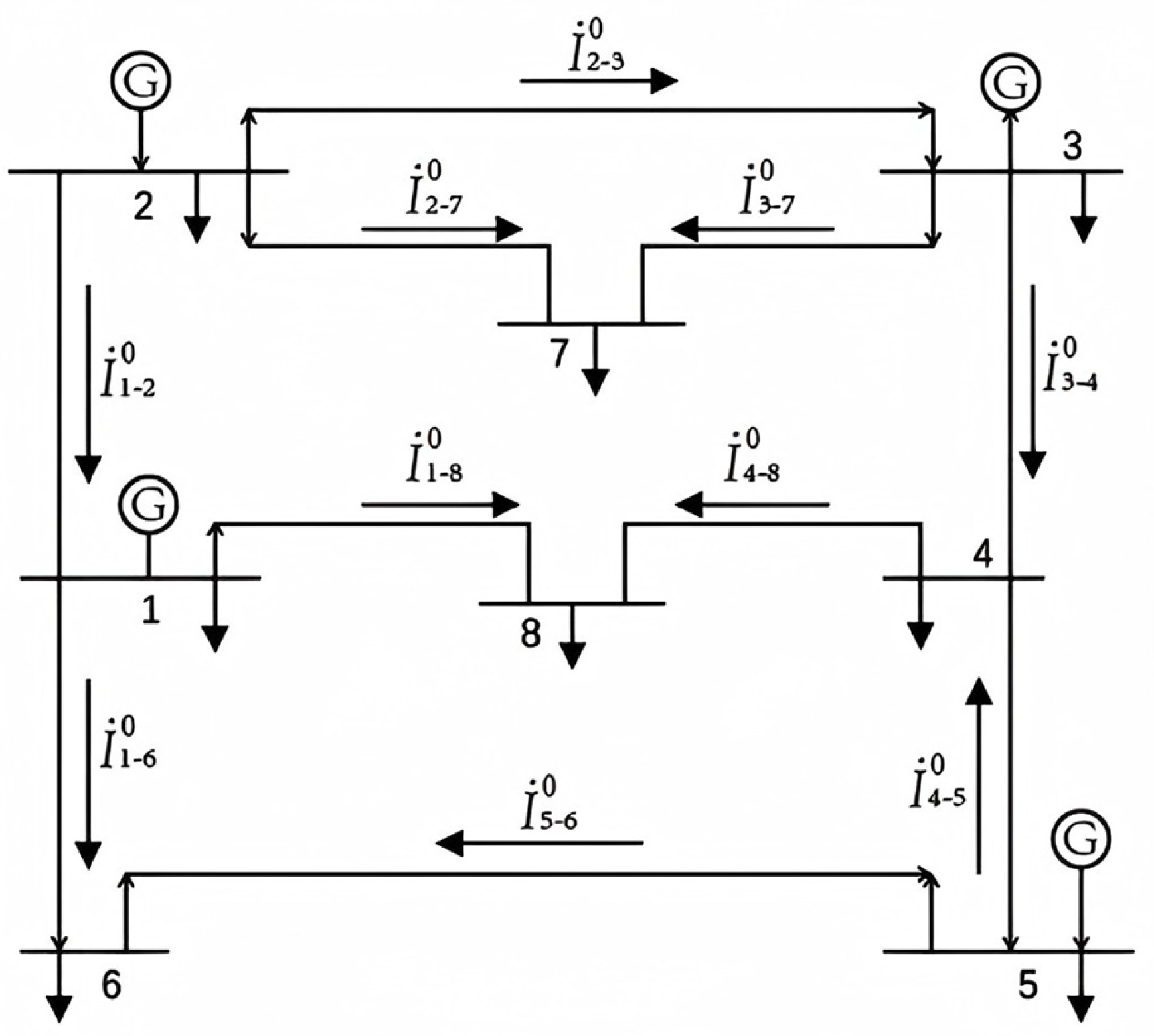
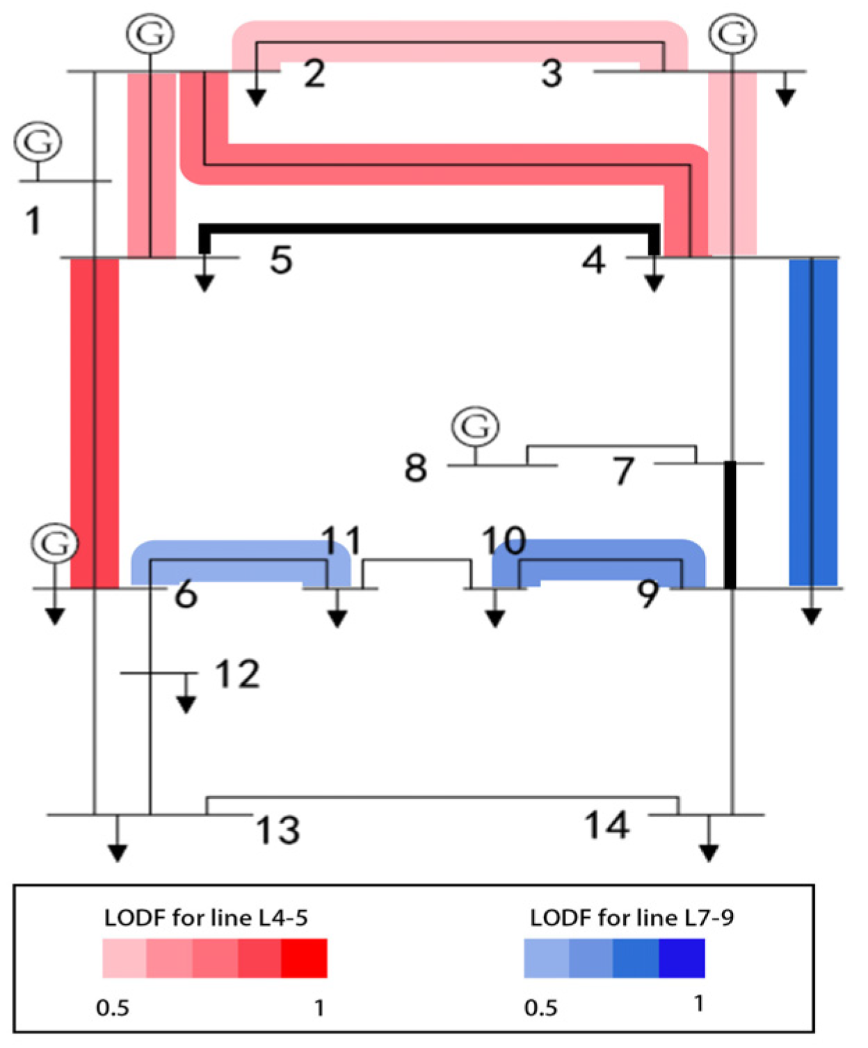
According to power flow theory, upon the removal of an overloaded branch, power flow undergoes redistribution across the entire power network. Specifically, only a limited number of branches are significantly impacted by such power flow transfer, and this set of heavily affected lines is defined as a transmission section [10]. In essence, power flow transfer refers to the phenomenon whereby the power initially transmitted by a tripped overloaded line is redistributed to other lines within the power grid. To illustrate the aforementioned characteristics, the 8-bus system is adopted as a case study, with relevant results presented in Figure 1.

Assuming that line $L_{2-3}$ is tripped as a result of an overload fault, the power flow originally transmitted by this line will be transferred to adjacent lines. These adjacent lines will absorb the transferred power flow to maintain the stability of overall power transmission with the total power flow magnitude unchanged. For the purpose of subsequent analysis, two key assumptions are made: first, the line outage exerts no influence on generators and loads, such that the active power output of each generating unit and the magnitude of each system load remain unchanged; second, the power system is treated as a linear system with nonlinear components neglected. Based on the fundamental superposition theorem for linear systems, the calculation method for the power flow of other lines in the system subsequent to the tripping of $L_{2-3}$ is derived as follows: the power flow magnitude of line $L_{i-j}$ is equal to the sum of its initial power flow magnitude and the power flow transferred thereto from the faulted line $L_{2-3}$. The specific calculation formula is presented below:

$${\dot{I}}_{i-j}={\dot{I}}_{i-j}^0+\Delta {\dot{I}}_{i-j}$$

(1)

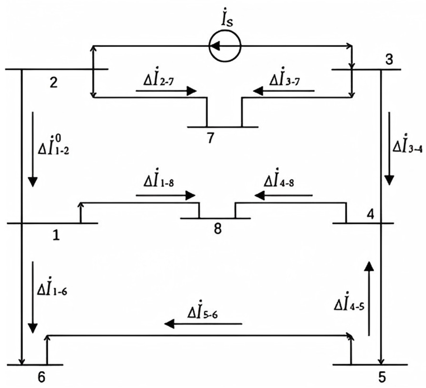
In the equation, ${\dot{I}}_{i-j}$ represents the current in line $L_{i-j}$ after the faulted line is cleared, ${\dot{I}}_{i-j}^0$ denotes the current in $L_{i-j}$ before the faulted line is cleared, and $\Delta {\dot{I}}_{i-j}$ indicates the power flow transfer component redistributed to L_i-j after the faulted line is cleared. Taking the removal of line $L_{2-3}$ as an example, $\Delta {\dot{I}}_{i-j}$ can be calculated by modeling the system as an equivalent passive network; the faulted line $L_{2-3}$ is replaced with a current source that has the same magnitude but in the opposite direction to the original current. The power flow is then recalculated under this equivalent condition, as shown in Figure 2.

In the equivalent network of the power flow transfer component in the figure, the transfer current $\Delta I_{i-j}$ for line $L_{i-j}$_j satisfies

$$△{\dot{I}}_k={\displaystyle \frac{△{\dot{U}}_i-△{\dot{U}}_j}{Z_{ij}}}$$

(2)

In the equation, the impedance parameter $Z_{ij}$ of line $L_{i-j}$, along with the voltage increment parameters $△{\dot{U}}_i$ and $△{\dot{U}}_j$, form the fundamental variables. In engineering calculations, to simplify the computation, $Z_{ij}$ is often reduced to its reactance component $X_{ij}$. Under this simplification, the voltage increments and the line current variable can be substituted by $△{\dot{U}}_i$, $△{\dot{U}}_j$, and ${\dot{I}}_{ij}$, respectively. Based on this, the expression for the transferred current component of line $L_{i-j}$ can be derived as follows:

$$\Delta I_k={\displaystyle \frac{\Delta U_i-\Delta U_j}{X_{ij}}}$$

(3)

Neglecting the impact of network losses and other environmental conditions, and considering that reactance is the main factor while ignoring the impact of resistance, the network can be converted into a DC network equivalent model. Let the current $I$ in the network be the current flowing through each loop including the current source. Therefore, the current variable $L_{i-j}$ of branch is the sum of the currents of each branch, that is, where $U$ is the set of loops through which the current passes through branch $L_{i-j}$.

From the perspective of power system topology, when an overloaded branch trips, branches with smaller electrical distance exhibit greater susceptibility to power flow transfer, while those with larger electrical distance demonstrate lower responsiveness. Therefore, branches exhibiting significant susceptibility to power flow transfer are concentrated in those that maintain a small electrical distance from the tripped branch and can constitute a closed loop together with it. Notably, branches with smaller electrical distance are predominantly distributed within loops characterized by lower loop impedance [15,16]. Consequently, the key to identifying the transmission section resides in the effective identification of loops, with lower loop impedance formed in conjunction with the tripped line.

This paper introduces the branch outage distribution factor [17] to reflect the degree of influence of other branches in the system by power flow transfer after a branch is removed. This refers to the percentage of the power flow change on another line $K$ to the initial power flow on line $L$ after line $L$ is disconnected. Its expression is

$$D_{k-l}={\displaystyle \frac{x_{k-l}/x_k}{1-x_{l-l}/x_l}}$$

(4)

$X_{k-l}$ is the mutual impedance between node $K$ and node $L$, and $X_{l-l}$ is the self-impedance of node $L$. $D_{k-l}$ is related to the network structure and the network’s own impedance and does not change easily under normal circumstances. When the network structure changes, $D_{k-l}$ will also change. Therefore, when a branch is removed due to a fault, $D_{k-l}$ needs to be recalculated to screen out key transmission sections. Compare whether $D_{k-l}$ of each branch included in the found top $K$ shortest paths are greater than the set value to screen out key transmission sections [18].

To find the top $K$ shortest paths, this paper uses the car relay algorithm. The car relay algorithm is analogous to Dijkstra’s algorithm and is developed to determine the shortest path between an origin node and a destination node. Specifically, the path is assessed with respect to assigned numerical weights, such as line reactance in power system applications. By simulating the traveling process of a vehicle, the algorithm adopts the remaining fuel level as a quantitative metric for assessing the path length. It regards nodes in the power network as stations, branches between nodes as routes, and the reactance of branches as the length of routes. A car is sent from the starting station to each adjacent station, and then a car is sent from this adjacent station to other adjacent stations. The fuel quantity of the car is the same as the fuel quantity when arriving at this station. This continues until it reaches the target station. Compare the remaining fuel quantity of each car arriving at the target station; the car with the most remaining fuel has taken the shortest route. Trace back the routes of the top $K$ cars to find the top $K$ shortest loops. Then, use the above branch outage distribution factor to screen out branches in the top $K$ shortest loops that meet the screening requirements. If its $D_{k-l}$ is greater than the set threshold (generally 0.2–0.3), the branch is a key transmission section. The values of $K$ and the threshold were determined as described in Reference [15].

3. Transmission Section Based on Grid Partitions

Power grid zoning refers to the process of partitioning an interconnected power network into multiple sub-regions in accordance with specific criteria. Specifically, these sub-regions exhibit a certain degree of homogeneity and relative independence in terms of electrical characteristics, geographical distribution, and functional positioning while maintaining necessary connections through tie lines and other means to collectively form an organic integrated system. From the perspective of electrical connectivity, nodes within the same partition feature short electrical distances, frequent power flow interactions, and close interconnections via high-voltage transmission lines; in contrast, the electrical connectivity between different partitions is relatively weak, thereby confining the scope of fault propagation.

Among existing approaches, zoning methods based on graph theory and electrical distance represent the most classical categories. These methods abstract the power system into a graph structure, where generator and load nodes are defined as vertices and transmission lines as edges. Notably, electrical distance serves as one of the core bases for power grid zoning. Path-finding algorithms such as Dijkstra’s algorithm are utilized to calculate the electrical distance between nodes, with nodes featuring close electrical connectivity grouped into the same sub-region [19]. Additionally, spectral clustering algorithms (e.g., the K-means algorithm) leverage eigenvectors of the graph’s Laplacian matrix for dimensionality reduction, followed by clustering in the reduced-dimensional space. This category of algorithms can effectively identify the community structure of the power network and has emerged as a mainstream zoning approach [20]. Reference [21] presents a Key Transmission Section (KTS) search method based on an improved clustering algorithm, wherein a modified normalized clustering algorithm is employed for power grid partitioning. To address the challenge of determining the criticality of numerous transmission sections identified between partitions, a security risk index is designed and adopted.

Generally, power grid zoning is predominantly underpinned by the high-voltage grid, with 500 kV substations serving as the core of each partition [22]. Specifically, other nodes that maintain close electrical connectivity with these core substations constitute a cohesive set, which is defined as a single partition. Consistent with this framework, this paper also adopts 500 kV substations as central vertices and employs the Car Relay Algorithm for power grid zoning. The tie lines between adjacent partitions are designated as the initial key transmission sections. The detailed implementation steps are outlined as follows:

(1)

Convert the power system into a weighted graph and form an adjacency matrix.

A graph is a network composed of edges and nodes, which can be understood as a collection of lines associated with nodes and used to study complex relationships between nodes, denoted as $G\left(V, E\right)$. $V$ is the set of points, and $E$ is the set of edges. Let $E\left(G\right)$ be the edge set of Graph $G$, and the expression of $E$ is

$$E=\left\{e_i| e_i=\langle v_p,v_q\rangle ,v_p,v_q\in V\right\}$$

(5)

Notably, the identification of key transmission sections in a power system is associated with the system’s topological structure and is independent of the physical characteristics of individual components within the network. That is to say, when focusing on the power system’s topological structure, it suffices to abstract the system into a graph, enabling the application of graph theory methods for analyzing key section identification. Specifically, each bus in the power system is modeled as a node in the graph and each transmission line as an edge. A weighted graph is defined as a graph where each edge is assigned a specific numerical value (e.g., length, reactance). Consistent with this modeling approach, this paper adopts reactance as the edge weight.

(2)

Simplify the grid structure to eliminate dangling nodes and construct a weighted adjacency matrix.

The power grid structure is first simplified by removing power supply lines and ground connections. Specifically, buses in the power system are modeled as graph nodes, while transmission lines or transformers are treated as graph edges. The reactance of lines or transformers is adopted as the edge weight, thereby converting the original system into a weighted topological structure. Subsequently, dangling nodes in the network are eliminated, as illustrated in Figure 3.

For example, in graph $E\left(G\right)$, assign a weight with special significance to all lines in graph $G$. The weighted adjacency matrix $A$ is a set of relationships obtained from the weighted graph and expressed in matrix form. The element representation method of the weighted adjacency matrix $A$ is as follows:

$$a_{i-j}=\left\{\begin{array}{cc}0\hfill & i=j\hfill \\ w_{i-j}\hfill & i\ne j \mathrm{and} i,j \mathrm{related}\hfill \\ \infty \hfill & i\ne j \mathrm{and} i,j \mathrm{are} \mathrm{not} \mathrm{related}\hfill \end{array}\right.$$

(6)

In the formula, $W_{i-j}$ represents the weight of the line between $v_i$ and $v_j$. The adjacency matrix is a square matrix. If the network has n nodes, an $n\times n$ square matrix will be formed. The weighted adjacency matrix $A$ is a symmetric matrix, and elements $a_{i-j}$ and $a_{ji}$ are equal. Due to the sparsity of connections between nodes, the form matrix is also a sparse matrix. This paper uses reactance as the weight. The adjacency matrix elements are defined as follows: $a_{i-j}$ equals $W_{i-j}$ when nodes $v_i$ and $v_j$ are connected, and zero when they are not. The diagonal elements $a_{i-i}$ is all set to zero, as a node does not connect to itself. Through this matrix, the topological relationships and connection strengths between nodes in the network are clearly represented.

Once the weighted adjacency matrix is constructed, subsequent analysis can be performed. For instance, the overall connectivity of the network can be assessed through the calculation of the total weight of all edges, which aids in understanding the tightness of interconnections among network nodes. Furthermore, the importance of individual nodes can be evaluated by analyzing the sum of weights of their connected edges—nodes with a higher sum of connected edge weights typically play a more critical role in network operation and power flow.

Additionally, this weighted adjacency matrix can be applied to a range of network analysis algorithms. In path-finding algorithms, for example, the weights can denote costs or distances, enabling the matrix to assist in identifying optimal paths between distinct nodes in the network. In clustering algorithms, the matrix facilitates the grouping of nodes with similar connectivity patterns, which in turn supports the identification of sub-networks or functional groups within the broader network.

(3)

Introduce the impedance correction factor [17] $F_{ij}$; then,

$$Z_{ij}^{\prime }=Z_{ij}/{\left(U_{ij}/U_0\right)}^2=Z_{ij}/F_{ij}$$

(7)

In the formula, U represents the reference voltage level of the line, $Z_{ij}$ represents the initial reactance of the line, and $U_{i-j}$ represents the voltage level of line $L_{i-j}$.

After the preparation process, the car relay algorithm begins, and the specific algorithm process is as follows:

(1)

First, multiple starting stations, denoted as $s_1, s_2, s_3,\dots , s_n$, are selected as the departure points, which also serve as the center points of each partition. In this study, 500 kV substations are chosen as the starting stations. From each starting station, fully fueled vehicles are dispatched to adjacent, labeled stations. Upon arrival at each adjacent station $t$, the vehicles temporarily pause while a distance evaluation is performed.

(2)

Relative distance calculation and distance-based judgment: Once a vehicle arrives at a station t, the relative distance d between the origin station s and station t is computed. If the calculated distance $D$ is less than a predefined threshold distance $D_m$, the vehicle is shut down and parked at station $t$, and the process proceeds to the next relay step. Conversely, if the distance d exceeds $D_m$, it indicates that station t lies beyond the acceptable range from the starting station $s$, and thus no vehicle remains parked at it.

(3)

Proceeding to the next relay: At this stage, the adjacent stations of the current station are categorized into upstream and downstream stations. Upstream stations are defined as those from which vehicles have previously arrived at the current station, while the remaining neighboring stations are classified as downstream stations. Vehicles are then dispatched from the current station to each of the downstream stations. It is required that every eligible station send vehicles to its downstream stations as specified.

(4)

Recalculating relative distance and performing distance judgment: After a vehicle reaches a downstream station, the distance between that station and the original starting station $s$ is computed again. The iterative judgment process described in step (2) is repeated.

(5)

Relay repetition: The relay process continues iteratively until no new station is found with a distance $D$ less than $D_m$. This indicates that all nodes within the radius $D_m$ from the starting station s have been identified and assigned to the partition. All stations where a vehicle eventually parks are considered part of the sub-region centered at the starting station $s$.

(6)

Re-correction process: In cases where a station falls within the search radii of two or more starting stations, the distances between that station and each relevant starting station are recalculated. The station is then assigned to the partition whose starting station is nearest. Additionally, verification is conducted to ensure all nodes have been traversed. If any nodes are missed, possibly due to an inappropriate choice of $D_m$, the shortest path and distance from each initial station to the omitted node are computed, and the node is assigned to the partition with the smallest shortest-path distance.

The zoning process and precautions are shown below:

(1)

Convert the power grid topology into a weighted topological graph according to the aforementioned steps.

(2)

Due to the introduction of the impedance correction parameter, the reactance values between system nodes at different voltage levels must be converted to equivalent values at a unified voltage level for calculation, so as to determine the specified electrical distance $D_m$ for the power system.

(3)

Select the number of partitions and the starting substations, and perform a search based on the Vehicle Relay Model algorithm, traversing all nodes.

(4)

Determine whether a node lies within the specified electrical distance $D_m$; check if the node falls within the prescribed range.

(5)

Adjust and supplement nodes that do not meet the conditions or were missed, ensuring all nodes are processed.

(6)

Output the resulting qualified substations and partition information.

After the partitioning is complete, the inter-regional tie lines are identified as the initial key sections.

4. Simulation Result Analysis

This section presents a comprehensive experimental validation of the proposed critical transmission section identification methodology through systematic case studies on standard test systems. The research employs a structured analytical approach that integrates theoretical modeling with empirical simulations to evaluate method effectiveness. The overall technical road map encompasses three critical phases: grid partitioning based on electrical characteristics, vulnerability assessment using CLODF, and comparative analysis of critical transmission sections.

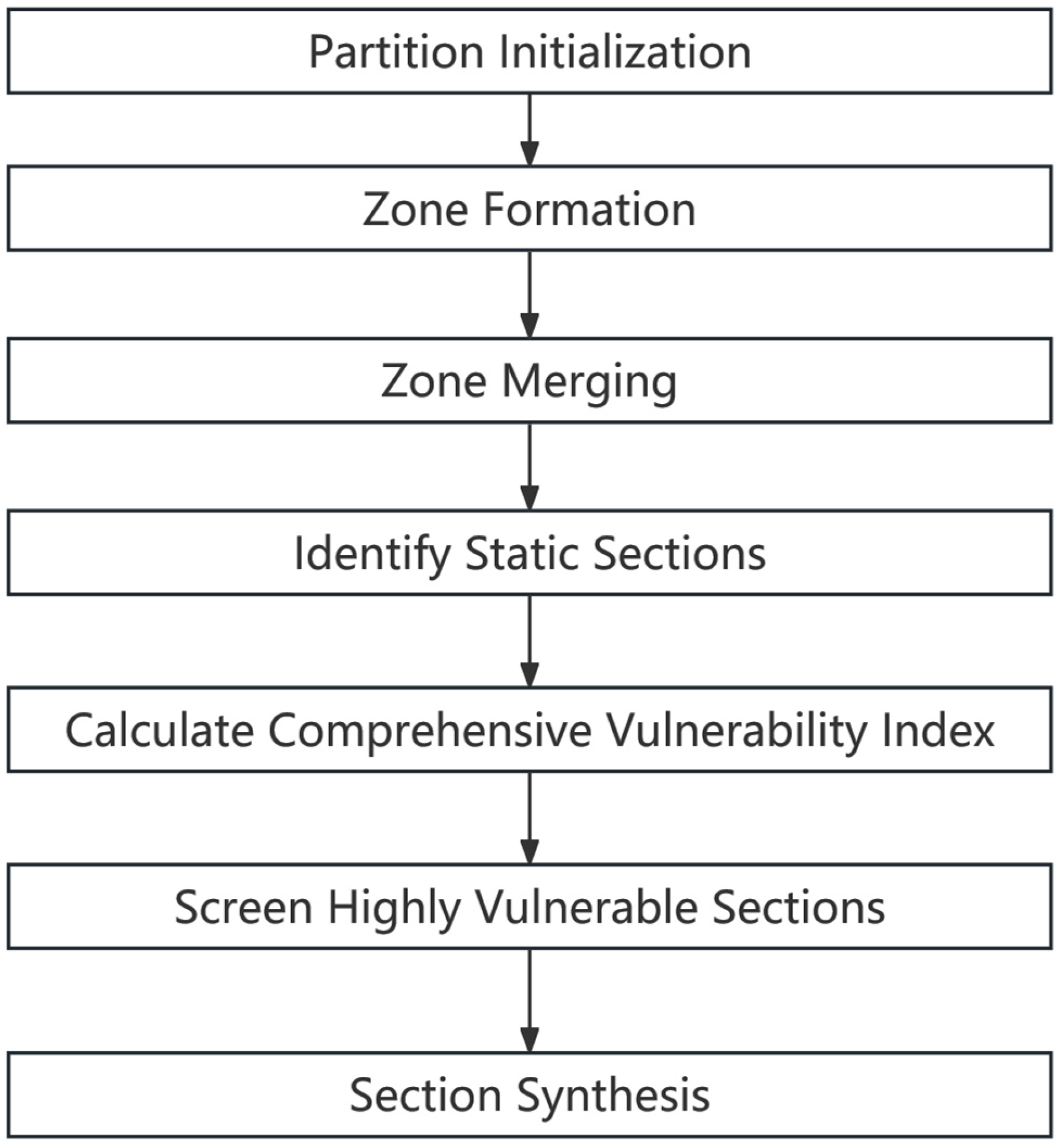
The following flowchart Figure 4 illustrates the methodology of this paper.

• Partition Initialization: High-voltage generator buses (e.g., 500 kV substations) are selected as central nodes or “anchors” for each partition.
• Zone Formation: The car relay algorithm is employed to partition the power grid by assigning all nodes within a predefined electrical distance threshold from a central node into the same region. In cases where a node falls within the threshold distance of multiple central nodes, it is allocated to the partition associated with the closest central node based on the minimal electrical distance.
• Zone Merging: Partitions whose central generator nodes are in very close electrical proximity may be merged into a larger area to reflect their strong coupling.
• Identify Static Sections: Upon completion of partitioning, all tie-lines connecting the different areas are automatically identified as the initial set of “transmission sections”. These represent the fundamental corridors for inter-area power exchange.
• Calculate Comprehensive Vulnerability Index: For each line in the system, CLODF is calculated. This metric quantifies the aggregate impact on a specific line when outages occur on other lines within the same partition it connects, effectively measuring its overall vulnerability to power flow transfers.
• Screen Highly Vulnerable Sections: The identified “static sections” and the screened “dynamic sections” are to be consolidated and deduplicated. Furthermore, individual analyses should be conducted for lines exhibiting larger CLODF to pinpoint those lines exerting a major influence on power flow distributions.

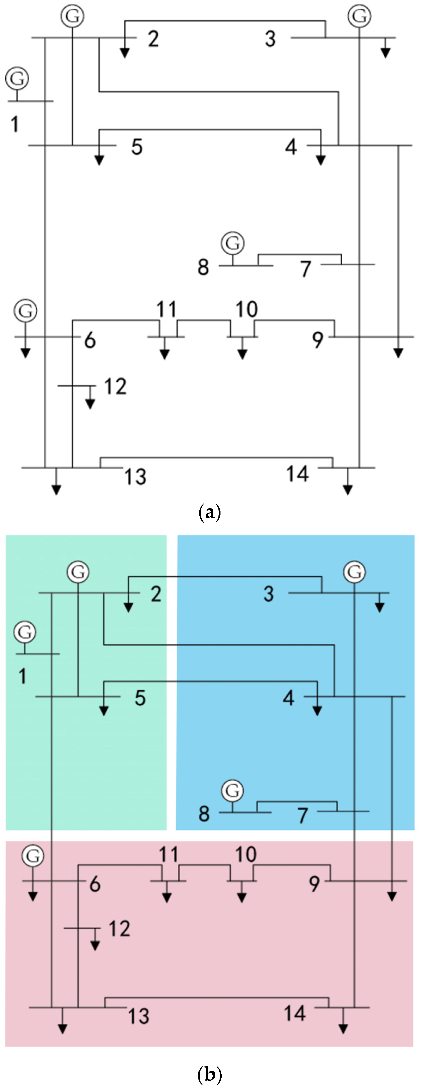
Simulations were conducted using the IEEE 14-bus system, the network structure of which is shown in the figure below. In the IEEE 14-bus system, generator buses are located at [1, 2, 3, 6, 8]. Therefore, we designated these generator buses as central nodes for partitioning. The results show that Bus 1 and Bus 2, which are in close electrical proximity, can be clustered into one area. Similarly, Bus 3 and Bus 8 can form another area due to their short electrical distance. The simulation algorithm yielded three distinct regions: [1, 2, 5], [3, 4, 7, 8], and [6, 11, 10, 9, 12, 13, 14]. The partition results are shown in Figure 5 and

Table 1. Schematic table of power system zoning results.

Partition Serial Number	Include Node
1	1, 2, 5
2	3, 4, 7, 8
3	6, 11, 10, 9, 12, 13, 14

.

Transmission sections $L_{2-3}$, $L_{2-4}$, $L_{5-4}$, $L_{4-9}$, $L_{7-9}$, $L_{5-6}$.

Based on the definition of the Line Outage Distribution Factor provided in Section 2, $D_{k-l}$ refers to the percentage change in power flow on line $K$ after the outage of line $L$, relative to the initial power flow on $L$. This paper introduces a comprehensive line outage distribution factor $D_K$ to quantify the degree of power flow changes on a specific line $K$ when other lines in the system are outaged. $D_K$ is calculated by summing the absolute values of all $D_{k-l}$ terms, where $L$ represents all other lines within the same partitions that line $K$ spans. For example, if line $K$ is $L_{2-3}$ (a tie-line between Partition 1 and Partition 2), then $L_1$, $L_2$, …, $L_n$ would encompass all lines within Partition 1 and Partition 2.

Table 2. Schematic table of comprehensive line outage distribution factors for the IEEE 14-Bus system.

Line	From Bus → To Bus	Comprehensive Line Outage Distribution Factor
1	1 → 2	2.663
2	1 → 5	2.663
3	2 → 3	2.3513
4	2 → 4	3.1412
5	2 → 5	3.0697
6	3 → 4	2.3513
7	4 → 5	7.8637
8	4 → 7	4.4962
9	4 → 9	2.653
10	5 → 6	4.8327
11	6 →11	4.989
12	6 → 12	2.6129
13	6 → 13	5.0926
14	7 → 8	0
15	7 → 9	4.4962
16	9 → 10	4.989
17	9 → 14	3.9246
18	10 → 11	4.989
19	12 → 13	2.6129
20	13 → 14	3.9246

presents the comprehensive line outage distribution factors calculated for the IEEE 14-bus system.

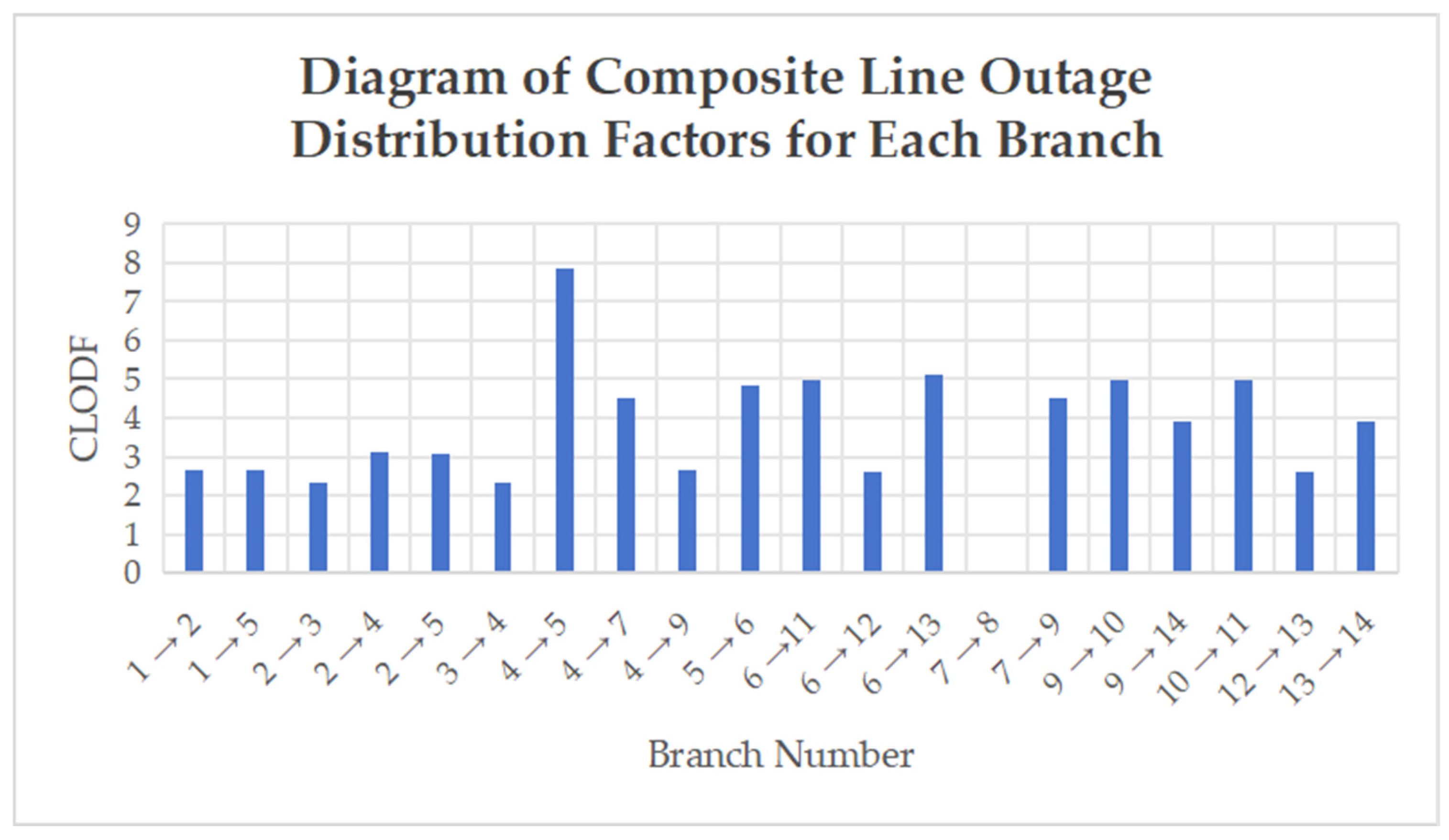
In order to see the size of the CLODF more clearly and intuitively, the table content is made into a bar chart as shown in Figure 6.

As can be observed from the table, the magnitude of the comprehensive line outage distribution factor varies across different branches. The CLODF value for branch $L_{7-8}$ is zero because Bus 8 is connected to the system solely through this branch and is directly linked to a generator, resulting in an $X_{k-l}$ value of zero. Hence, its CLODF is zero.

A higher CLODF value indicates greater vulnerability of the branch and a stronger influence on other branches. By comparing the CLODF values of the transmission interface branches—$L_{2-3}$, $L_{2-4}$, $L_{5-4}$, $L_{4-9}$, $L_{7-9}$, and $L_{5-6}$—it is evident that $L_{5-4}$ has the highest CLODF, making it the most vulnerable and the most significantly affected by outages of other branches. Therefore, this branch requires prioritized monitoring. In contrast, branch $L_{2-3}$ has a relatively low CLODF and can be excluded from being classified as a critical transmission section.

Analyzing branch $L_{4-5}$, which exhibits the highest comprehensive line outage distribution factor, the top five lines with the greatest LODF values relative to it were selected through calculation, yielding the following

Table 3. Schematic table of line outage distribution factors for branches $L_{4-5}$.

Branch	LODF
L5–6	0.8435
L2–4	0.6761
L2–5	0.6050
L2–3	0.5153
L3–4	0.5153

.

Then, branch $L_{7-9}$ is analyzed, and the branch cutoff distribution factor of each branch is calculated, as shown in

Table 4. Schematic table of line outage distribution factors for branches $L_{7-9}$.

Branch	LODF
L4–9	0.6426
L9–10	0.3779
L6–11	0.3779

.

This point is clearly evident, as illustrated in Figure 7:

According to the definition of the line outage distribution factor—which is the ratio of the change in power flow on a specified line to the pre-outage power flow on the outage line—the outage of line $L_{5-6}$ has the greatest impact on the power flow of line $L_{4-5}$, followed by $L_{2-4}$, $L_{2-5}$, $L_{2-3}$, and $L_{3-4}$, respectively. The line that has the most influence on branch $L_{7-9}$ is $L_{4-9}$, followed by $L_{9-10}$ and $L_{6-11}$.

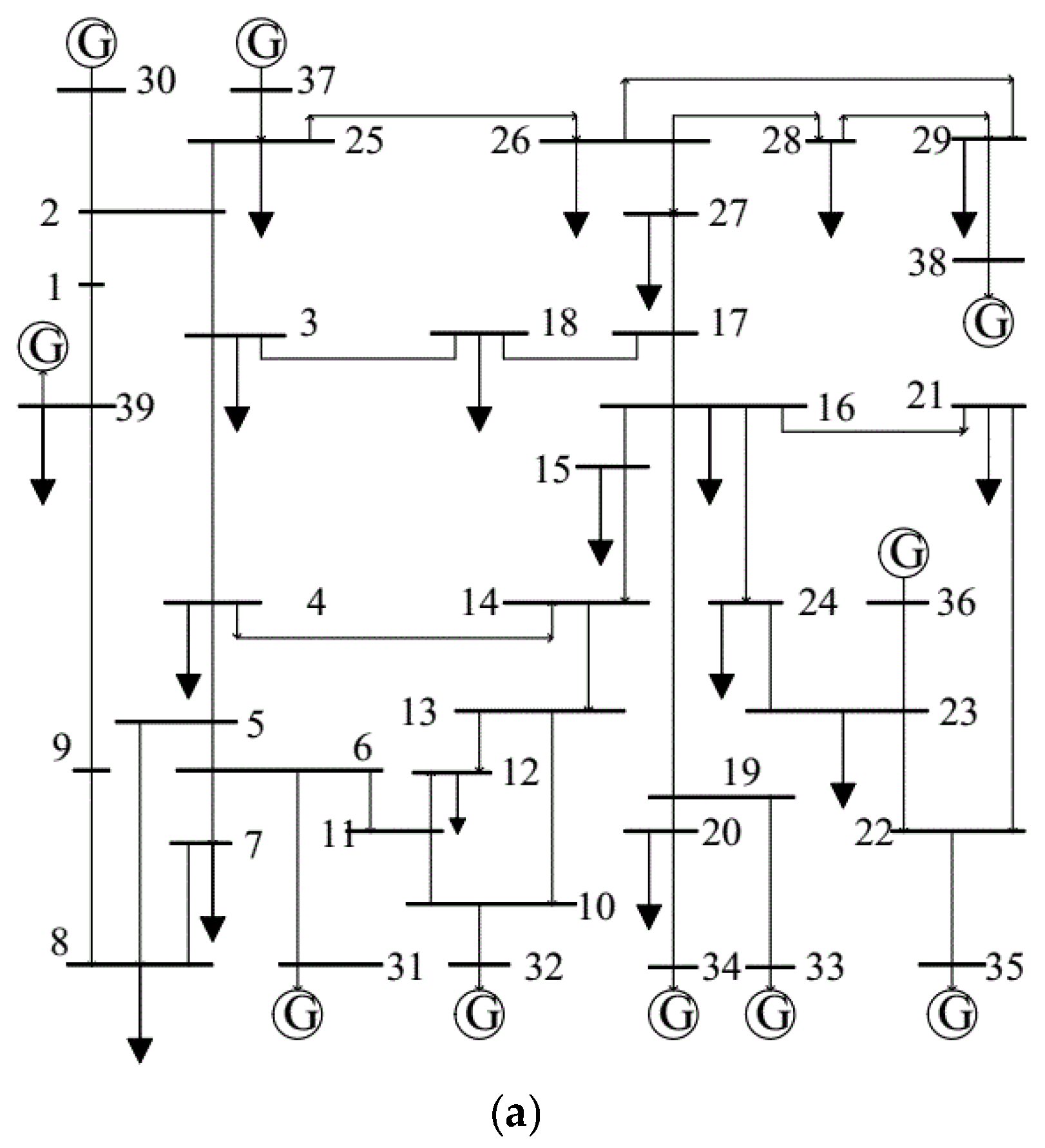
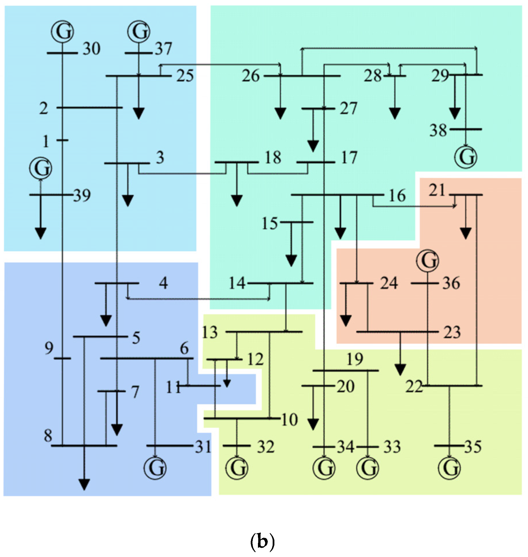
In the IEEE 39-bus system, the generator buses are located at [30, 37, 31, 32, 34, 33, 36, 35, 38]. Therefore, these generator buses were selected as the central nodes for partitioning. The partitioning results indicated that buses 37, 30, and 39, being in close electrical proximity, can be grouped into one area. Similarly, buses 32, 33, 34, and 35 can form another area due to their short post-partitioning electrical distance; the simulation yielded the following five regions: [30, 37, 25, 2, 1, 39, 3], [26, 27, 18, 17, 15, 14, 16, 21, 39, 29], [21, 36, 23, 24], [35, 22, 33, 34, 20, 19, 13, 12, 10, 32], and [31, 8, 7, 9, 5, 6, 4, 11].

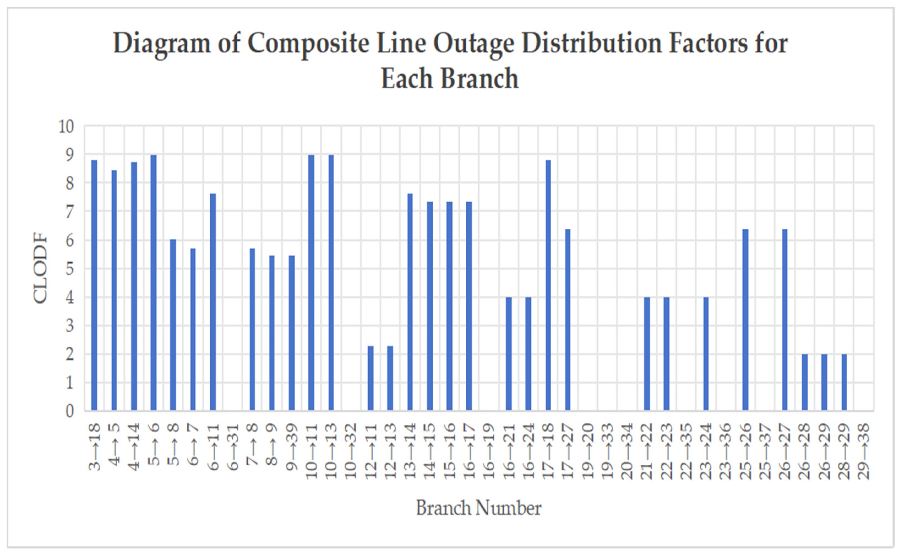
Through the power grid zoning result in Figure 8a, the inter-regional tie-line transmission interfaces are identified as $L_{39-9}$, $L_{3-4}$, $L_{4-14}$, $L_{3-18}$, $L_{25-26}$, $L_{16-21}$, $L_{16-24}$, $L_{22-23}$, $L_{21-22}$, $L_{16-19}$, $L_{14-13}$, $L_{11-10}$, and $L_{11-12}$. By calculating the comprehensive line outage distribution factors for each line, the following

Table 5. Schematic table of CLODFS for the IEEE 39-Bus system.

Line	From Bus → To Bus	Comprehensive Line Outage Distribution Factor
1	1 → 2	5.4567
2	1 → 39	5.4567
3	2 → 3	8.885
4	2 → 25	6.3713
5	2 → 30	0
7	3 → 18	8.809
8	4 → 5	8.4375
9	4 → 14	8.7277
10	5 → 6	8.9864
11	5 → 8	6.0017
12	6 → 7	5.7089
13	6 → 11	7.6271
14	6 → 31	0
15	7 → 8	5.7089
16	8 → 9	5.4567
17	9 → 39	5.4567
18	10 → 11	8.9926
19	10 → 13	8.9926
20	10 → 32	0
21	12 → 11	2.2852
22	12 → 13	2.2852
23	13 → 14	7.6271
24	14 → 15	7.3413
25	15 → 16	7.3413
26	16 → 17	7.3413
27	16 → 19	0
28	16 → 21	4
29	16 → 24	4
30	17 → 18	8.809
31	17 → 27	6.3713
32	19 → 20	0
33	19 → 33	0
34	20 → 34	0
35	21 → 22	4
36	22 → 23	4
37	22 → 35	0
38	23 → 24	4
39	23 → 36	0
40	25 → 26	6.3713
41	25 → 37	0
42	26 → 27	6.3713
43	26 → 28	2
44	26 → 29	2
45	28 → 29	2
46	29 → 38	0

is obtained.

As shown in the Table 5 and Figure 9, line L10-11 has the highest comprehensive line outage distribution factor, followed in descending order by $L_{3-18}$, $L_{4-14}$, $L_{3-4}$, $L_{13-14}$, $L_{25-26}$, $L_{9-39}$, $L_{16-21}$, $L_{16-24}$, $L_{21-22}$, $L_{22-23}$, and $L_{16-19}$. A higher CLODF value indicates that the line is more susceptible to impacts from outages of other lines and should be prioritized for monitoring.

Therefore, in power system operation and management strategies, these lines with high CLODF values should be designated as key monitoring priorities. Operational protocols should emphasize enhanced surveillance of their operational status, with a focus on analyzing interdependencies with other lines in the network. Regular assessments of their vulnerability to cascading outages should be conducted, and contingency plans should be developed to address potential risks. By prioritizing these critical lines in system monitoring and risk management frameworks, operators can proactively mitigate the impact of line outages and maintain overall grid stability.

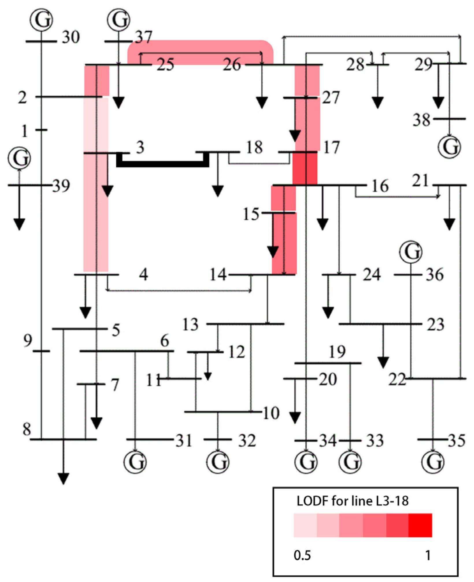
Analyzing branch $L_{3-18}$, which exhibits the highest comprehensive line outage distribution factor, the top nine lines with the greatest LODF values relative to it were selected through calculation, yielding the following

Table 6. Schematic table of line outage distribution factors for branches $L_{3-18}$.

Branch	LODF
L16–17	0.7823
L14–15	0.7826
L15–16	0.7826
L17–27	0.7360
L25–26	0.7360
L26–27	0.7360
L25–2	0.7360
L3–4	0.6116
L2–3	0.5898

:

This Figure 10 clearly identifies the lines that significantly impact the power flow on $L_{3-18}$, namely $L_{16-17}$, $L_{14-15}$, $L_{15-16}$, $L_{17-27}$, and $L_{25-26}$. To minimize the chance of omission, the search for other potentially influential lines can be continued. Protecting $L_{3-18}$ can thus be achieved by monitoring these critical associated lines.

Following the identification of transmission interfaces through system zoning, we calculated their comprehensive line outage distribution factors. The line most susceptible to system disturbances, identified by the highest comprehensive LODF, was then analyzed to determine which other lines have the greatest impact on it. This analysis allows for targeted prevention and enhanced monitoring of these critical linkages.

After obtaining the lines with significant impact, we further evaluated the potential risks associated with each critical linkage. By simulating various outage scenarios, we quantified the extent to which the failure of each line would affect the power flow on L3-18. This risk assessment provided a clear picture of the vulnerabilities in the power system.

5. Discussion

The findings of this study represent a valuable integration and advancement within the existing research framework. Traditional critical section identification methods typically follow two independent technical approaches: the first involves static grid partitioning based on graph theory and electrical distance to identify sections formed by inter-regional connection lines; the second utilizes the shortest path algorithm with power flow transfer coefficients to search for power flow transfer paths during specific faults. Our method innovatively combines these perspectives by not only obtaining static partitioned sections reflecting long-term grid operation structures through an improved relay algorithm but also introducing a comprehensive branch outage distribution factor as a quantitative indicator. This approach accurately characterizes dynamic power flow transfer characteristics and section vulnerability under fault disturbances. Single-method limitations may exist; focusing solely on partitioning might overlook fault-driven weak-links, while concentrating on fault paths could neglect critical inter-regional connection channels. The integration of high-proportion renewable energy sources has significantly increased grid operation uncertainty and volatility, rendering traditional empirical-based static security analysis methods inadequate for addressing these challenges. This research provides technical support for building multi-objective new power systems. At the planning level, the high-vulnerability sections identified offer scientific decision-making basis for grid reinforcement, energy storage deployment, and flexible resource optimization, enhancing investment efficiency. At the operational level, this method serves as the core of real-time security early warning and prevention/control systems, effectively boosting the grid’s resilience against unknown disturbances and cascading failures while ensuring power supply reliability. In the market dimension, these clear partitioning of sections and power flow relationships provides transparent and efficient quantitative tools for designing transmission right allocation and congestion management mechanisms, facilitating cross-regional renewable energy integration. Future research can be deepened in multiple directions. Algorithmically, artificial intelligence technologies like machine learning and graph neural networks could be introduced to improve computational efficiency and adaptability in the real-time analysis of ultra-large-scale grids. Application-wise, the focus should be on deep integration with early online security warnings and prevention/control systems, developing intelligent decision-making that dynamically updates critical section sets and adapts to different operational modes. The research scope should expand to include hybrid AC/DC grid scenarios and complex scenario safety analyses considering extreme weather and multiple faults.

6. Conclusions

Confronted with the persistent challenges of high computational complexity and low operational efficiency in traditional power grid partitioning methods for large-scale systems, along with the inherent difficulty in achieving a balanced identification of critical transmission sections that incorporates both static grid infrastructure and dynamic fault-induced risks, this research proposes an integrated methodology. The approach systematically combines grid partitioning with a vulnerability-based analysis for section identification. The process initiates with the application of the Car Relay Algorithm to achieve a rational grid partition, whereby inter-area tie-lines are identified as the preliminary set of transmission sections, thus establishing a structural foundation for subsequent analysis. A pivotal mechanism for quantifying line vulnerability under contingency scenarios is then established through the introduction of CLODF. This factor serves as a critical metric, where an elevated CLODF value signifies a line’s heightened susceptibility to power flow transfers resulting from the outage of other lines, thereby enabling the precise identification of fault-driven dynamic critical sections. This methodology effectively captures vulnerable links within power flow transfer pathways during faults, successfully remedying the common deficiency of overlooking dynamic risk points in analyses that rely solely on static grid assessment. Consequently, it provides substantial technical support for mitigating the risk of cascading failures and enhancing the overall security and stability of modern power systems.

Future research will focus on extending the proposed method to real-world large-scale power grids, incorporating extreme weather and multi-fault scenarios to enhance practical applicability. Artificial intelligence technologies will be integrated to optimize algorithmic efficiency and enable real-time performance in ultra-large-scale systems. Further efforts will deepen compatibility with online security early-warning systems to support dynamic updates of critical transmission sections. Additionally, the method’s application will be expanded to distribution networks, broadening its engineering relevance and operational value.