Generalized Non-Convex Non-Smooth Group-Sparse Residual Prior for Image Denoising

Abstract

Image denoising is a classic yet challenging problem in low-level image processing. Traditional image denoising approaches using convex regularized prior (e.g., $L_1$-norm) often bring bias problems. To address this issue, a novel prior model based on a family of non-convex functions and group sparsity residual (GSC) prior constraint for image denoising is studied. We propose a generalized non-convex GSC prior model for the image denoising problem. We first utilize the group-sparse representation (GSR) before exploiting image prior information. Specifically, to further improve the image denoising performance of the GSC prior model, we employ several typical non-convex surrogate functions for the sparsity constraint. Then, a fast and efficient thresholding algorithm is proposed to minimize the resulting optimization problem. The experimental results have demonstrated that our proposed method can achieve the best reconstruction results compared with other image denoising approaches.

1. Introduction

Image denoising is a classic yet popular low-level image processing problem, whose purpose is to reconstruct the latent clean image $\mathbf{x}$ from the noisy observation $\mathbf{y}=\mathbf{x}+\mathbf{n}$, where $\mathbf{n}$ is usually defined as additive Gaussian white noise [1,2,3,4]. Mathematically, image denoising can be successfully addressed via the following optimization problems:

$$\underset{\mathbf{x}}{min}f\left(\mathbf{y},\mathbf{x}\right)+\lambda \Re \left(\mathbf{x}\right)$$

(1)

where $f(\mathbf{y},\mathbf{x})$ denotes the data term, $\Re \left(\mathbf{x}\right)$ denotes the regularizer, and the non-negative parameter $\lambda$ is used to balance the data term and regularizer.

In the past decade, image denoising problems have achieved great progress [1,2,3,5,6]. Mathematically, image denoising is an ill-posed problem; thus, the prior model plays a crucial role in improving the image denoising performance. The most widely used models include the sparsity model [7], non-local self-similar model [8,9,10,11], wavelet transform model, and Markov random field model [12]. In addition, deep-learning-based denoising approaches are also increasingly proposed. Among them, convolution neural networks (CNN) [13,14] and recursive neural networks (RNN) [13,14] are mostly used for image denoising. With the maturity of deep learning theory, various network structures have been applied to image denoising and have achieved excellent results [13,14,15]. Although deep-learning-based approaches for image denoising have achieved promising progress, their drawbacks are obvious, e.g., requiring clean, large-scale, labeled datasets for training.

In recent years, sparsity has been increasingly used for image denoising [16,17,18]. Elad et al. [16] used K-SVD for dictionary learning to obtain a sparse dictionary, then performed image denoising in units of image blocks. In 2010, Mairal et al. [17] proposed the LSSC algorithm, which uses dictionary learning to mine local sparsity in the domain and combines non-local methods to explore non-local sparsity. To take advantage of the sparsity between image blocks, Zhang et al. [18] proposed the concept of group sparsity in 2014 by combining several similar image blocks into groups and using the group as the basic unit of sparse representation, then using the SBI algorithm to solve the cost function to improve the robustness of the model. In 2017, Lin et al. [19] proposed an image reconstruction algorithm based on a sparse representation of an adaptive structure group. This algorithm can adaptively adjust the criteria for selecting similar image blocks according to the image’s own structure and regional characteristics, thus improving the performance of model reconstruction.

Non-local structure self similarity (NSS) is one of the most popular image denoising prior models in recent years [20,21,22]. For the model of NSS, the non-local means (NLM) is employed to exploit the NSS characteristics of the image for image denoising, which is an improvement on the traditional neighborhood filtering method and takes into account the self-similar nature of the image. It makes full use of the redundant information in the image and can preserve the details of the image to the greatest extent while denoising. Buades et al. [8,23] first proposed the method of non-local means. This method first determines the weight according to the similarity between the pixel area to be processed and other similar point neighborhoods, and then uses the weight to calculate the gray value of the pixel, which is the weighted average of the gray values of all pixels in the image. Since then, new and improved algorithms have been proposed continuously. Kervrann et al. [24] made improvements in the selection of similar blocks, which improved the denoising performance. Goossens et al. [25] proposed a dual scoring function to calculate the weights, which improves the calculation accuracy of the similarity between similar blocks and improves the denoising performance. Inspired by NLM, Dabov et al. [5] proposed the BM3D method to solve the problem of image denoising. The BM3D algorithm uses collaborative filtering in the three-dimensional transform domain, and the denoising performance reaches an unprecedented height.

In addition, the low-rank property can also be used as prior knowledge for image denoising [26]. The WNNM method proposed by Gu et al. also uses the low-rank attribute of the image. Since this model ignores low-rank properties, the effect of image noise reduction can be achieved through low-rank clustering. Dong et al. [27] proposed applying the low-rank attributes of images as prior knowledge to image compressed sensing, which showed good performance and further improved the denoising ability based on the NSS model. Fen et al. [28] proposed an image compression sensing model based on low-rank priors. Based on the traditional image low-rank model, the Schatten-p norm was used instead of the weighted kernel norm to improve the reconstruction ability of the model [29]. Chen et al. [30] used the low-rank property of images to design non-local low-rank regularization terms, and at the same time, selected m-estimation to achieve robust image compression sensing denoising. This algorithm not only has good denoising performance but also has excellent robustness. Zhang et al. [31] applied the sparsity and low rank of this image to MRI image denoising and achieved good results. Recently, residual prior-based models have shown their promising advantages in various image processing tasks, such as sparsity residual prior [7,32], rank residual prior [33], and deep residual feature in network [34].

The so-called convex optimization method uses a convex function as a penalty function, and the most commonly used ones include $L_1$ and $L_2$ norms. The non-convex optimization method is to choose a non-convex function as the penalty function, and the most used one is $L_p\left(p<1\right)$. By computing sparse vectors from noisy images, both convex optimization methods and non-convex optimization methods can achieve the goal, but both types of methods have their advantages and disadvantages. Among them, the convex optimization method can better guarantee the convergence of the algorithm. Non-convex optimization methods can obtain more sparse solutions.

In practical applications, the problem (1) is typical NP-hard, which is difficult to solve directly. Usually, the $L_1$ norm and $L_2$ norm are used for convex optimization solutions. However, convex optimization often cannot obtain a perfect solution because a perfect approximation of the rank function cannot be obtained. In order to better approximate the rank function, many non-convex surrogate functions have been proposed, including the -norm [35], the smooth clipped absolute deviation (SCAD) [36], the logarithm [37], the minimax concave penalty (MCP) [38], and the exponential type penalty (ETP) [39].

In this paper, we propose a method for non-convex optimization groups with sparse residual-constrained models. First, we transform the image denoising problem into a residual minimization problem using group-sparse residuals, which simplifies the computation and understandability. To better approximate the value function, we choose a non-convex substitution function to replace the traditional convex substitution function, which improves the denoising performance of the model. Finally, to compare the performance of non-convex surrogate functions, we selected the five most commonly used non-convex surrogate functions for comparative experiments. The final experiment proves that the model not only has good denoising performance but also has high efficiency.

The rest of the paper is organized as follows: Section 2 presents some basics, including dictionary learning, group-sparse models, group-sparse residuals, and low-rank minimization models. In Section 3, a non-convex optimization group-sparse residual constrained model is proposed, and the model is solved. Section 4 presents the experiments and results and analyzes them. Section 5 summarizes the full text.

2. Related Work

In this section, we will briefly introduce some related work in image denoising, including group sparse representation, adaptive dictionary learning, and low-rank minimization theory.

2.1. Group Sparse Representation

Recently, the group sparsity prior has been popularly used for image denoising tasks, which has significantly improved image denoising performance [18,40]. For any image $\mathbf{x}$, there are n overlapping patches ${\mathbf{x}}_i$ with a size of $\sqrt{b}\times \sqrt{b}$; then we can search k patches in the $L\ast L$ sized searching windows based on the benchmarked ${\mathbf{x}}_i$ using the kNN method [41]. The patch set is defined by ${\mathbf{X}}_i=\left\{{\mathbf{x}}_{i1},{\mathbf{x}}_{i2},{\mathbf{x}}_{i3},\dots ,{\mathbf{x}}_{ik}\right\}$, where ${\mathbf{x}}_{ik}$ denotes the k-th patch similar to ${\mathbf{x}}_i$. If we define a representation dictionary ${\mathbf{D}}_i$ for each group ${\mathbf{X}}_i$, then ${\mathbf{X}}_i$ can be expressed as ${\mathbf{X}}_i={\mathbf{D}}_i{\mathbf{C}}_i$, where ${\mathbf{C}}_i$ denotes the group sparse vector.

2.2. Low-Rank Minimization

The low-rank approximation problem can be summarized as follows: given an input group $\mathbf{Y}\in {\mathbb{R}}^{M\times N}$, the purpose of the low-rank minimization method is to find a low-rank matrix $\mathbf{X}\in {\mathbb{R}}^{M\times N}$ through minimizing the objective function (e.g., data fidelity term and the constraint of the regularization term). In general, the low-rank minimization can be expressed as follows:

$$\widehat{\mathbf{X}}=\arg \underset{\mathbf{X}}{min}f(\mathbf{X},\mathbf{Y})+\lambda \Re \left(\mathbf{X}\right)$$

(2)

where $f\left(\mathbf{X}\right)$ denotes the loss function and $\Re \left(\mathbf{X}\right)$ denotes the low-rank constraint term with a non-negative weight $\lambda$. The most popular choice of $f(\mathbf{X},\mathbf{Y})$ is the squared loss: $f(\mathbf{X},\mathbf{Y})={\displaystyle \frac{1}{2}}{∥\mathbf{Y}-\mathbf{X}∥}_2^2$. In practical applications, low-rank minimization is a typical NP-hard problem, which is difficult to solve directly. The nuclear norm minimization (NNM) and weight nuclear norm minimization (WNNM) are two popular algorithms for approximation. In fact, however, the nuclear norm or weighted nuclear norm is not a perfect approximation of the rank function. Usually, the $L_1$-based nuclear norm is usually used to obtain a biased solution.

2.3. Adaptive Non-Local Dictionary Learning

Dictionary learning is also called sparse dictionary coding. The goal of dictionary learning is to extract the most essential features of objects by reducing the interference of other insignificant transactions on the target. The sparse model is consistent with the goal of dictionary learning, which is to remove useless information and retain the most essential and important information. Therefore, the quality of dictionary creation is closely related to the sparsity of the model. Given a group ${\mathbf{Y}}_i$, we have [42,43]

$${\mathbf{Y}}_i={\mathbf{D}}_i{\mathbf{A}}_i$$

(3)

where ${\mathbf{D}}_i$ denotes the group dictionary and ${\mathbf{A}}_i$ is the corresponding coefficient matrix. Then, the process of dictionary learning can be expressed as follows:

$$({\mathbf{D}}_i,{\mathbf{A}}_i)=arg\underset{{\mathbf{D}}_i,{\mathbf{A}}_i}{min}{\displaystyle \frac{1}{2}}{∥{\mathbf{Y}}_i-{\mathbf{D}}_i{\mathbf{A}}_i∥}_F^2+\lambda {∥{\mathbf{A}}_i∥}_0$$

(4)

Since $L_0$-norm is difficult to solve, it is usually relaxed by the popular $L_1$ regular term. Firstly, randomly select samples from the original sample ${\mathbf{Y}}_i$ as the initial value of ${\mathbf{D}}_i$, and initialize ${\mathbf{A}}_i$ to $\mathbf{0}$. Then, iteratively update ${\mathbf{D}}_i$ and ${\mathbf{A}}_i$ respectively, and finally obtain the dictionary ${\mathbf{D}}_i$ with the best sparsity.

However, the dictionary learning method via (4) is usually complicated and inefficient. In this paper, we introduce a novel approach to achieve the non-local dictionary $\mathbf{D}$ via SVD technology [18,44]. Considering the group ${\mathbf{Y}}_i$, the SVD of ${\mathbf{Y}}_i$ is

$${\mathbf{Y}}_i^{\prime }={\mathbf{U}}_i{\mathbf{\Sigma }}_i{\mathbf{V}}_i^T=\sum _{k=1}^j{\mathbf{\delta }}_{i,k}{\mathbf{u}}_{i,k}{\mathbf{v}}_{i,k}^T$$

(5)

Thus the dictionary atom can be obtained by

$${\mathbf{d}}_{i,k}={\mathbf{u}}_{i,k}{\mathbf{v}}_{i,k}^T.$$

(6)

Therefore, the non-local dictionary for each group is formed by

$${\mathbf{D}}_i=\left[{\mathbf{d}}_{i,1},{\mathbf{d}}_{i,2},\cdots ,\mathbf{d}j\right].$$

(7)

3. Proposed Method

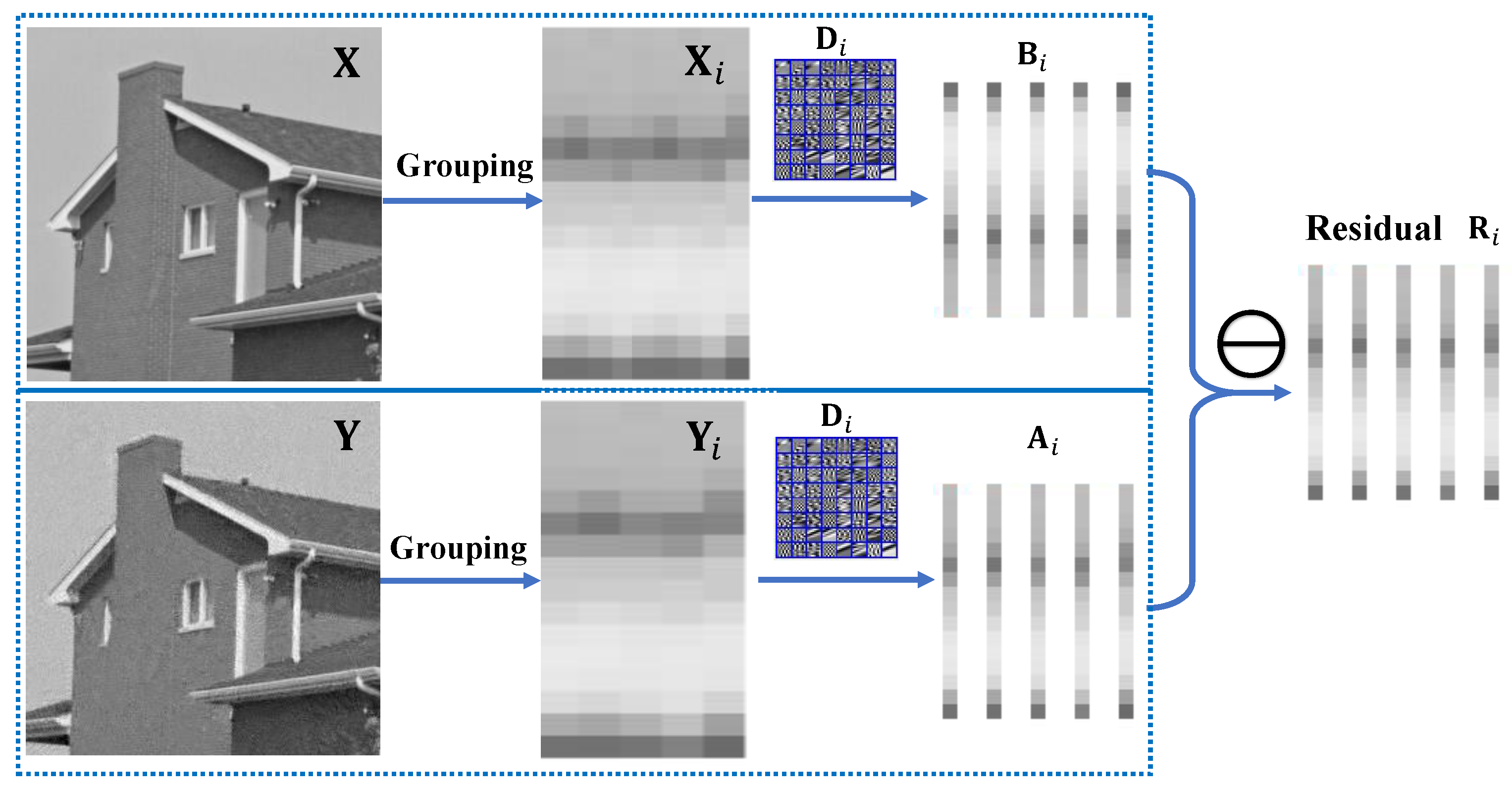
3.1. Group Sparse Coefficient Residual

For image $\mathbf{x}$ and its corresponding group ${\mathbf{X}}_i$, if we give a dictionary ${\mathbf{D}}_i$, then the group ${\mathbf{X}}_i$ can be sparsely represented by solving the following optimization problem,

$${\mathbf{B}}_i=arg\underset{{\mathbf{B}}_i}{min}\left\{{∥{\mathbf{X}}_i-{\mathbf{D}}_i{\mathbf{B}}_i∥}_F^2+\lambda {∥{\mathbf{B}}_i∥}_0\right\},$$

(8)

where ${\mathbf{B}}_i$ denotes the i-th group sparse coefficient for group ${\mathbf{X}}_i$. In practical applications for image denoising tasks, for the noisy image $\mathbf{y}$ and its corresponding group ${\mathbf{Y}}_i$, considering the fact that ${\mathbf{Y}}_i$ and ${\mathbf{X}}_i$ can share the same dictionary ${\mathbf{D}}_i$, the corresponding optimization problem for the i-th group sparse coefficient can be modeled as

$${\mathbf{A}}_i=arg\underset{{\mathbf{A}}_i}{min}\left\{{∥{\mathbf{Y}}_i-{\mathbf{D}}_i{\mathbf{A}}_i∥}_F^2+\lambda {∥{\mathbf{A}}_i∥}_0\right\}$$

(9)

where ${\mathbf{A}}_i$ denotes the i-th group sparse coefficient for group ${\mathbf{Y}}_i$. Thus, group sparse coefficient residual [32,33] can be described as

$${\mathbf{R}}_i={\mathbf{A}}_i-{\mathbf{B}}_i$$

(10)

To better understand the group sparse coefficient residual, Figure 1 presents the flowchart of the group sparse coefficient residuals.

3.2. Residual Prior-Based Generalized Non-Convex Non-Smooth Low-Rank Minimization

The residual ${\mathbf{R}}_i$ defined in Equation (10) can indicate the difference between ${\mathbf{A}}_i$ and ${\mathbf{B}}_i$. Correspondingly, considering the low-rank minimization problem in Equation (2), the residual prior-based low-rank approximation can be formulated as

$${\widehat{\mathbf{X}}}_i=\arg \underset{\mathbf{X}i}{min}f\left({\mathbf{Y}}_i,{\mathbf{X}}_i\right)+\lambda \Re \left({\mathbf{R}}_i\right).$$

(11)

To address the optimization problem, the popular model is

$${\widehat{\mathbf{A}}}_i=arg\underset{{\mathbf{X}}_i}{min}\left\{{∥{\mathbf{Y}}_i-{\mathbf{D}}_i{\mathbf{A}}_i∥}_2^2+\lambda {∥{\mathbf{R}}_i∥}_p\right\}$$

(12)

where $0<p\le 1$.

To better approximate the rank of the matrix ${\mathbf{X}}_i$, many non-convex alternative functions have been proposed. The most commonly used one is the $l_p$-norm [35]. In this paper, we employ a family of non-convex non-smooth functions to regularize the group residual, including the $l_p$-norm [35], the smooth clipped absolute deviation (SCAD) [36], the Logarithm [37], the minimax concave penalty( MCP) [38], and the exponential type penalty (ETP) [39]. These non-convex substitution functions are described in

Table 1. Five popular non-convex surrogate functions and their super-gradients.

Penalty	Formula $\mathit{\rho }\left(\mathit{x}\right)$	Super-Gradient $\mathit{\partial }\mathit{\rho }\left(\mathit{x}\right)$
$L_p$	$\lambda {\theta }^p$	$\left\{\begin{array}{cc}\infty & x=0\\ \lambda p{x}^{p-1}& x>0\end{array}\right.$
SCAD	$\left\{\begin{array}{c}\lambda xx\le \lambda \\ {\displaystyle \frac{-x^2+2\gamma \lambda x-{\lambda }^2}{2\left(\gamma -1\right)}}\lambda <x\\ {\displaystyle \frac{{\lambda }^2\left(\gamma +1\right)}{2}}x>\gamma \lambda \end{array}\right.\le \gamma \lambda$	$\left\{\begin{array}{cc}\lambda & x\le \lambda \\ {\displaystyle \frac{\gamma \lambda -x}{\gamma -1}}& \lambda <x\\ 0& x>\gamma \lambda \end{array}\right.\le \gamma \lambda$
Logarithm	${\displaystyle \frac{\lambda }{log\left(\gamma +1\right)}}log\left(\gamma x+1\right)$	${\displaystyle \frac{\lambda \gamma }{\left(\gamma x+1\right)log\left(\gamma +1\right)}}$
MCP	$\left\{\begin{array}{cc}\lambda x-{\displaystyle \frac{x^2}{2\gamma }}& x<\gamma \lambda \\ {\displaystyle \frac{1}{2}}\gamma {\lambda }^2& x\ge \gamma \lambda \end{array}\right.$	$\left\{\begin{array}{cc}\lambda -{\displaystyle \frac{x}{\gamma }}& x<\gamma \lambda \\ 0& x\ge \gamma \lambda \end{array}\right.$
ETP	${\displaystyle \frac{\lambda }{1-exp\left(-\gamma \right)}}\left(1-exp\left(-\gamma x\right)\right)$	${\displaystyle \frac{\lambda \gamma }{1-exp\left(-\gamma \right)}}exp\left(-\gamma x\right)$

. Then our proposed group sparse residual prior-based non-convex non-smooth low-rank minimization can be formulated as

$${\widehat{\mathbf{A}}}_i=\arg \underset{{\mathbf{X}}_i}{min}\left({\displaystyle \frac{1}{2}}{\parallel {\mathbf{Y}}_i-{\mathbf{D}}_i{\mathbf{A}}_i\parallel }_2^2+\lambda \Re \left({\mathbf{R}}_i\right)\right)$$

(13)

According to earlier work [10,11], we have the following relationship for the group, e.g., ${\mathbf{X}}_i^{\prime }={\mathbf{U}}_i{\mathbf{\Sigma }}_i{\mathbf{V}}_i^T={\sum }_{k=1}^j{\mathbf{\delta }}_{i,k}{\mathbf{u}}_{i,k}{\mathbf{v}}_{i,k}^T$. Moreover, according to the definition of dictionary, it is easy to find that its atoms can be achieved by ${\mathbf{d}}_{i,k}={\mathbf{u}}_{i,k}{\mathbf{v}}_{i,k}^T$. Therefore, if we replace ${\mathbf{D}}_i{\mathbf{A}}_i$ with ${\mathbf{X}}_i$, the optimization problem in Equation (13) can be equal to the following problem:

$${\widehat{\mathbf{X}}}_i=\arg \underset{{\mathbf{X}}_i}{min}\left({\displaystyle \frac{1}{2}}{\parallel {\mathbf{Y}}_i-{\mathbf{X}}_i\parallel }_2^2+\lambda \Re \left({\mathbf{R}}_i\right)\right).$$

(14)

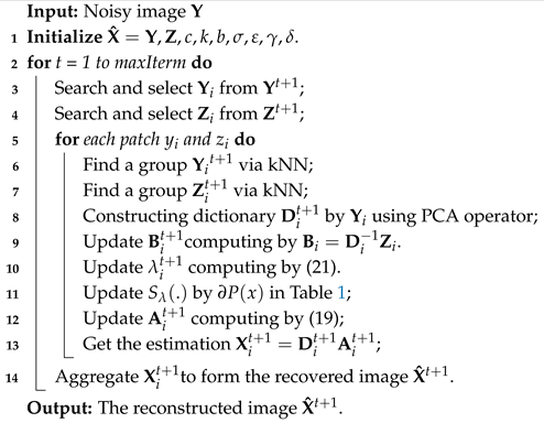
3.3. Image Denoising Application

To achieve good denoising performance, the group sparse residual ${\mathbf{R}}_i$ should be as small as possible. In this paper, our generalized non-convex non-smooth residual prior-driven image denoising can be modeled as

$$\widehat{\mathbf{\alpha }}=\arg \underset{\mathbf{\alpha }}{min}\left({\displaystyle \frac{1}{2}}{\parallel \mathbf{y}-\mathbf{d}\mathbf{\alpha }\parallel }_2^2+\lambda \sum _{i=1}^n\Re \left({\mathbf{A}}_i-{\mathbf{B}}_i\right)\right)$$

(15)

Let $\mathbf{x}=\mathbf{d}\mathbf{\alpha }$; we have

$$\widehat{\mathbf{x}}=\arg \underset{\mathbf{x}}{min}\left({\displaystyle \frac{1}{2}}{\parallel \mathbf{y}-\mathbf{x}\parallel }_2^2+\lambda \sum _{i=1}^n\Re \left({\mathbf{A}}_i-{\mathbf{B}}_i\right)\right)$$

(16)

According to [11,22], we have the following relationship with a large probability (close to 1) at each iteration:

$${\displaystyle \frac{1}{K}}\sum _{i=1}^n{\parallel {\mathbf{Y}}_i-{\mathbf{D}}_i{\mathbf{A}}_i\parallel }_{\mathbf{F}}^2={\displaystyle \frac{1}{N}}{\parallel \mathbf{y}-\mathit{d}\mathbf{\alpha }\parallel }_2^2$$

(17)

Therefore, our denoising problem can be converted into the following problem:

$${\widehat{\mathbf{X}}}_i=\arg \underset{{\mathbf{X}}_i}{min}\left({\displaystyle \frac{1}{2}}{\parallel {\mathbf{Y}}_i-{\mathbf{X}}_i\parallel }_2^2+\tilde{\lambda }\Re \left({\mathbf{A}}_i-{\mathbf{B}}_i\right)\right)$$

(18)

where $\tilde{\lambda }={\displaystyle \frac{\lambda K}{N}}$. In this work, we employed the surrogate algorithm [38] to solve (18), and we obtained the iterative formula:

$${\mathbf{A}}_i^{t+1}=S_{\tilde{\lambda }}({\mathbf{D}}_i^{-1}{\widehat{\mathbf{X}}}_i^t-{\mathbf{B}}_i^t)+{\mathbf{B}}_i^t$$

(19)

where $S_{\tilde{\lambda }}$ denotes the soft-thresholding operator, ${\mathbf{D}}_i$ is the principle component analysis (PCA) based dictionary of ${\mathbf{A}}_i$ [18,40]. In this paper, we adopt the non-convex surrogate function to solve $S_{\tilde{\lambda }}$. Here, we employ the popular $L_p$-norm as the relaxation function. According to the definition in Table 1, we have

$$S_{\tilde{\lambda }}=\left\{\begin{array}{cc}\infty & x=0\\ \tilde{\lambda }p{x}^{p-1}& x>0\end{array}\right.$$

(20)

where $\tilde{\lambda }$ is regularization parameter. To obtain better denoising performance, we set the parameter $\lambda$ to change adaptively according to [7,32].

$$\lambda ={\displaystyle \frac{c\ast 2\sqrt{2}\sigma n^2}{{\sigma }_i}}$$

(21)

where c is a small constant and is related to ${\mathbf{Y}}_i$. The ${\sigma }_i$ denotes the variance of the residual ${\mathbf{R}}_i$. In the iterative process, we choose the iterative regularization strategy to update the estimated variance of noise to improve the performance of the model,

$${\sigma }^{t+1}=\gamma \sqrt{({\sigma }^2-{∥\mathbf{Y}-{\widehat{\mathbf{X}}}^{t+1}∥}_2^2}$$

(22)

where $\gamma$ is a constant. After getting all ${\mathbf{A}}_i$, we can get the searched reconstruction blocks through

$${\widehat{\mathbf{X}}}_i={\mathbf{D}}_i{\widehat{\mathbf{A}}}_i.$$

(23)

The complete description of the proposed image denoising method is presented in Algorithm 1.

Algorithm 1: Non-convex Optimization Denoising Model Based on Group Sparse Residual Constraint

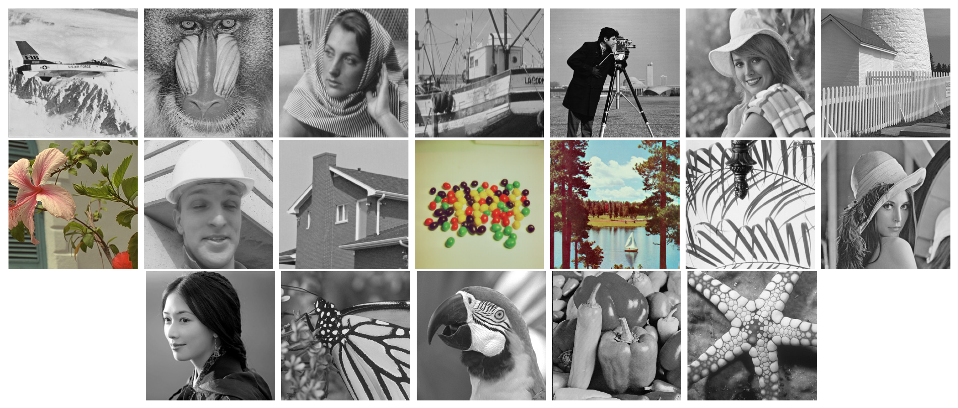
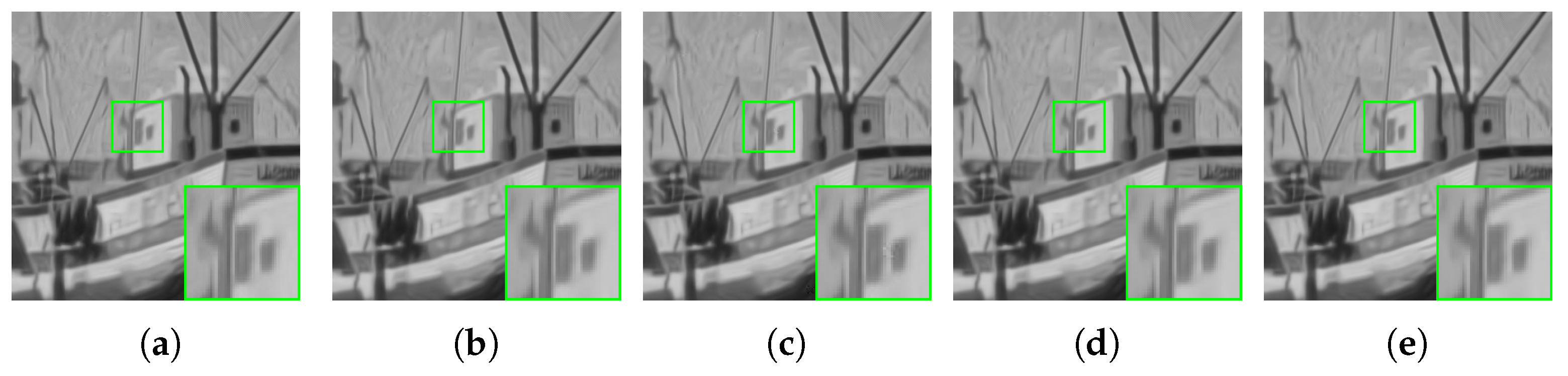
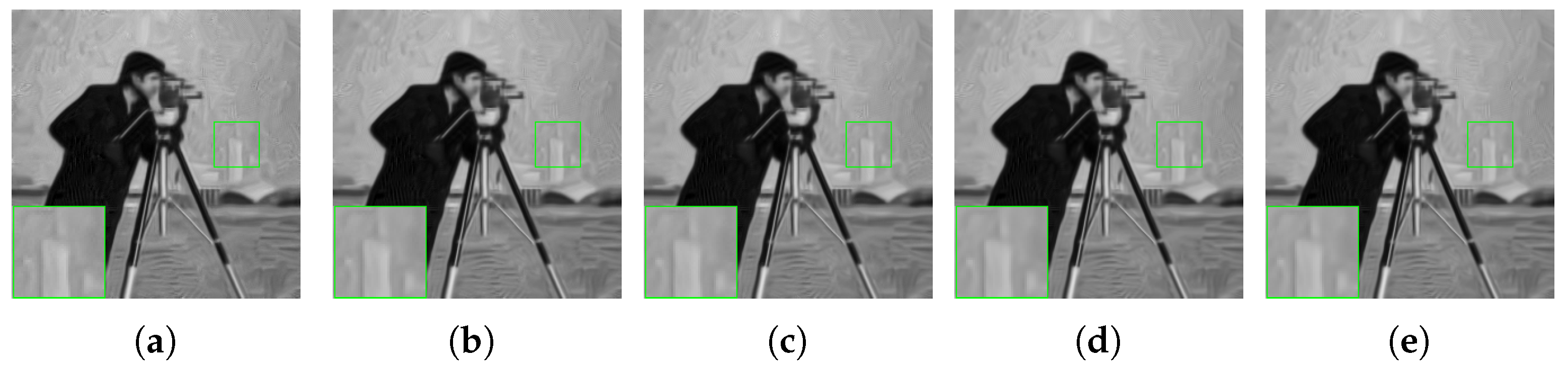
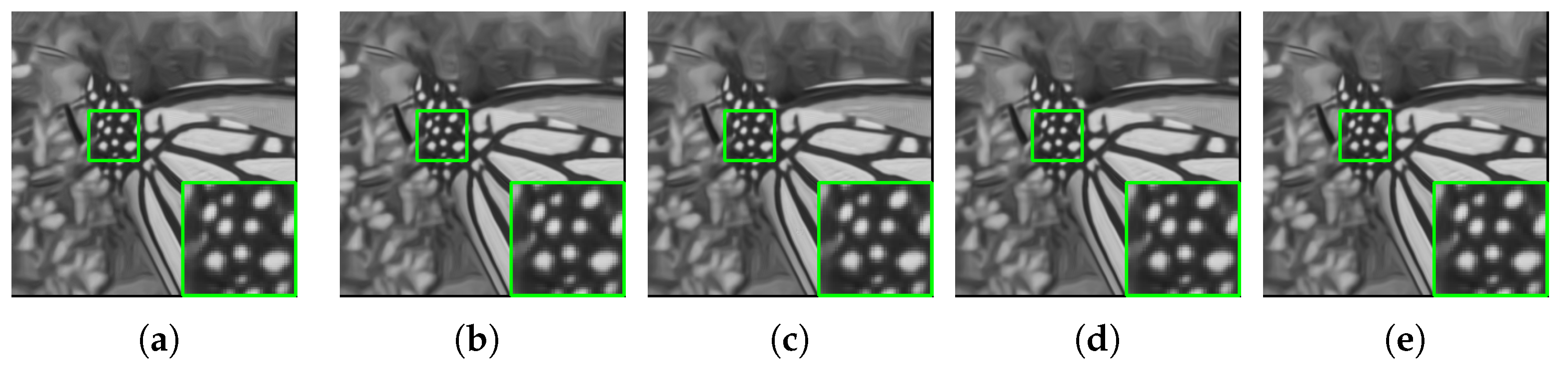
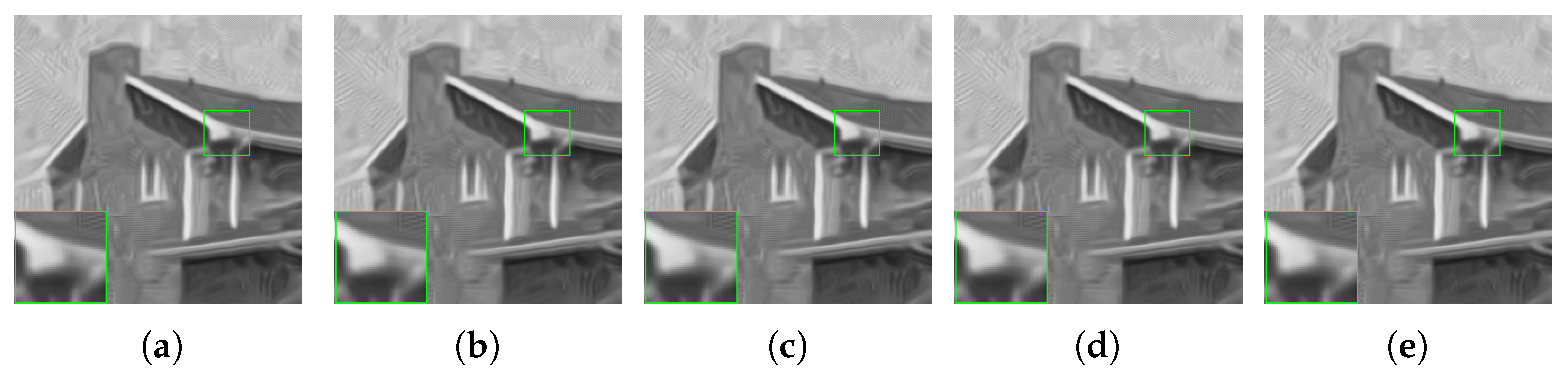
4. Experimental Results

In this section, extensive experimental results are presented to evaluate the image denoising performance of our proposed method. In this experiment, similar to the state-of-the-art methods [20,21,45], we also chose two widely used metrics to assess the objective and subjective quality of the reconstructed images, namely the peak signal-to-noise ratio (PSNR) and the Structural Similarity Index metric (SSIM), respectively. Note that PSNR is a commonly used indicator to measure signal/image distortion; though the evaluation results usually appear inconsistent with the supervisor’s feelings, it is still a valuable evaluation index. The SSIM evaluates images from three aspects: brightness, contrast, and structure. Therefore, neighborhood pixels have strong relevance, that is, the similarity of object structure information. The contrast peak signal-to-noise ratio is more complex with the intuitive effect observed by human vision, and it has symmetry, upper and lower bounds, and other properties. These two parameters are the most commonly used objective indicators to evaluate the quality of image restoration. They are defined as follows:

$$\mathrm{PSNR}=10{log}_{10}\left({\displaystyle \frac{{255}^2}{\frac{1}{3mn}{\sum }_{i=1}^3{∥{\widehat{X}}_i-M_i∥}_F^2}}\right)$$

(24)

where $M_i$ denotes the i-th channel of the original image, the default i is 1 for the grayscale image, and ${\widehat{X}}_i$ denotes the i-th channel of the repaired image. The size of the image is $m\times n$.

$$\mathrm{SSIM}({\widehat{X}}_i,M_i)={\displaystyle \frac{(2{\mu }_{{\widehat{X}}_i}{\mu }_{M_i}+c_1)({\sigma }_{{\widehat{X}}_i{M}_i}-c_2)}{({\mu }_{{\widehat{X}}_i}^2+{\mu }_{M_i}^2+c_1)({\sigma }_{{\widehat{X}}_i}^2+{\sigma }_{M_i}^2+c_2)}}$$

(25)

where ${\mu }_{{\widehat{X}}_i}$ is the average value of the gray value of pixels in the i-th channel of the repaired image, ${\mu }_{M_i}$ is the average value of the gray value of pixels in the i-th channel of the original image, ${\sigma }_{{\widehat{X}}_i}$ is the variance of ${\widehat{X}}_i$, ${\sigma }_{{\widehat{M}}_i}$ is the variance of $M_i$, and ${\sigma }_{M_i{\widehat{X}}_i}$ is the covariance of $M_i$ and ${\widehat{X}}_i$. $c_1$ and $c_2$ are constants used to maintain stability.

4.1. Effectiveness of Our Denoising Model

In this subsection, we will validate the effectiveness of our non-convex image denoising model by denoising noisy classic images and comparing it with some state-of-the-art denoising methods, including BM3D [5], NCSR [46], PGPD [47], A-NLS [45], and GSRC [7]. Note that BM3D, PGPD, and GSRC are three non-local-based image denoising methods. NCSR and A-NLS are two sparsity residual-based image denoising methods. Without loss of generality, the classic non-convex function of MCP is utilized to plug into our denoising model for denoising experiments. The size of the search window is related to the search efficiency of similar blocks. If the search window is too small, it will increase the search time and affect the efficiency; otherwise, similar blocks of the image may be missed, which will affect the image denoising performance of the denoising algorithm. To obtain the best denoising performance, suitable parameters are used for the proposed model. The searching window $W\times W$ is set to $25\times 25$, and the searching thresholding value is set to 0.2. The size of patch $b\times b$ is set to $6\times 6$, $7\times 7$, $8\times 8$, and $9\times 9$ for ${\sigma }_n\le 20$, $20<{\sigma }_n\le 50$, $50<{\sigma }_n\le 75$, and ${\sigma }_n>75$, respectively. The parameters of $\gamma$ and $\lambda$ are set as 1 × 10⁷ and 2.1, respectively. We chose 13 widely used test images (see Figure 2) to conduct image denoising experiments at four noise levels, i.e., Gaussian white noise with standard deviations $n=30,40,50,75$, and all the PSNR results are presented in

Table 2. The results of the images denoised using different methods.

${\mathit{\sigma }}_{\mathit{n}}=30$							${\mathit{\sigma }}_{\mathit{n}}=40$
Images	BM3D	NCSR	PGPD	A-NLS	GSRC	Ours	BM3D	NCSR	PGPD	A-NLS	GSRC	Ours
Airplane	28.49	28.34	28.63	28.59	28.68	28.97	26.88	26.78	27.12	27.10	27.21	27.51
Boats	29.33	29.05	29.32	29.34	29.42	29.65	27.76	27.52	27.90	27.80	27.97	28.17
Fence	28.19	28.14	28.13	28.43	28.39	28.65	26.84	26.76	26.91	27.11	27.16	27.41
Flower	27.97	27.88	28.11	28.20	28.21	28.45	26.48	26.35	26.68	26.75	26.84	27.11
Foreman	32.75	32.61	32.83	32.79	33.15	33.45	31.29	31.52	31.55	31.29	31.81	31.99
House	32.09	32.01	32.24	32.26	32.44	32.78	30.65	30.79	31.02	30.91	31.16	31.39
J. Bean	31.97	31.90	31.99	32.07	32.28	32.43	30.21	30.49	30.39	30.38	30.51	30.79
Lake	26.74	26.69	26.90	26.92	26.89	27.05	25.21	25.21	25.51	25.46	25.52	25.77
Leaves	27.81	28.04	27.99	28.37	28.56	28.78	25.69	26.20	26.29	26.69	26.82	27.02
Lena	29.46	29.32	29.60	29.50	29.66	29.89	27.82	28.00	28.22	28.00	28.16	28.43
Lin	30.95	30.65	30.96	30.83	30.92	31.21	29.52	29.27	29.73	29.39	29.47	29.61
Monarch	28.35	28.38	28.49	28.70	28.80	28.97	26.72	26.81	27.02	27.20	27.33	27.58
Starfish	27.66	27.69	27.67	27.89	28.02	28.29	26.06	26.17	26.21	26.36	26.53	26.72
${\mathit{\sigma }}_{\mathit{n}}=\mathbf{50}$							${\mathit{\sigma }}_{\mathit{n}}=\mathbf{75}$
Airplane	25.76	25.63	25.98	26.02	26.17	26.51	23.99	23.76	24.15	24.06	24.12	24.29
Boats	26.74	26.37	26.82	26.78	26.95	27.43	24.82	24.44	24.83	24.76	24.94	25.12
Fence	25.92	25.77	25.94	26.22	26.26	26.47	24.22	23.75	24.18	24.40	24.53	24.79
Flower	25.49	25.31	25.63	25.77	25.76	25.99	23.82	23.50	23.82	23.87	23.87	23.99
Foreman	30.36	30.41	30.45	30.46	30.77	30.70	28.07	28.18	28.39	28.54	28.75	28.94
House	29.69	29.61	29.93	30.13	30.45	30.74	27.51	27.16	27.81	28.06	28.59	28.83
J. Bean	29.26	29.24	29.20	29.26	29.58	29.87	27.22	27.15	27.07	27.12	27.29	27.42
Lake	24.29	24.15	24.49	24.44	24.44	24.65	22.63	22.48	22.76	22.61	22.61	22.82
Leaves	24.68	24.94	25.03	25.32	25.66	25.97	22.49	22.60	22.61	22.95	23.34	23.51
Lena	26.90	26.94	27.15	27.08	27.06	27.49	25.17	25.02	25.30	25.32	25.32	25.53
Lin	28.71	28.23	28.79	28.50	28.60	28.98	26.96	26.22	27.05	26.72	26.84	26.97
Monarch	25.82	25.73	26.00	26.12	26.25	26.54	23.91	23.67	24.00	24.11	24.35	24.65
Starfish	25.04	25.06	25.11	25.26	25.36	25.64	23.27	23.18	23.23	23.24	23.32	23.51

. From the results, we can find that our proposed method outperforms the other five competing methods in all cases in terms of PSNR values.

4.2. Generalization Validation of Different Penalties

In this subsection, we will study the generalization of our proposed non-convex denoising model by comparing the denoising performance of five non-convex functions under different standard deviations of Gaussian noise. Moreover, we selected 13 gray images a the size of 256 × 256 for the denoising test, as shown in Figure 2. These images are selected from the datasets Set12 and CSet8. The Cset8 datasets are all RGB images. In this experiment, those color images are converted into grayscale images. We select two normal levels with ${\sigma }_n=20$ and 100 for the experiments. The PSNR(dB)/SSIM values of all experimental results are shown in

Table 3. The denoised results of images corrupted by Gaussian noise with different standard deviations, i.e., ${\sigma }_n=20$ and 100.

Methods	ETP	Logarithm	Lp	MCP	SCAD
	${\mathit{\sigma }}_{\mathit{n}}=\mathbf{20}$
Airplane	25.35/0.7688	25.59/0.8047	25.50/0.7876	25.69/0.8202	25.67/0.8178
Baboon	23.41/0.5318	23.59/0.5428	23.60/0.5393	23.69/0.5500	23.68/0.5499
Barbara	26.86/0.8044	27.28/0.8277	27.28/0.8197	27.49/0.8372	27.46/0.8360
Boats	26.79/0.7770	27.18/0.8016	27.11/0.7913	27.34/0.8124	27.32/0.8113
Cameraman	24.25/0.7191	24.47/0.7624	24.44/0.7452	24.57/0.7836	24.55/0.7803
Elaine	28.24/0.8157	28.71/0.8412	28.72/0.8313	28.99/0.8536	28.95/0.8518
Foreman	30.80/0.8208	31.95/0.8691	31.87/0.8536	32.54/0.8907	32.45/0.8875
House	28.87/0.7637	29.64/0.8147	29.48/0.7956	29.95/0.8383	29.91/0.8346
Leaves	23.69/0.8565	23.84/0.8711	23.83/0.8662	23.91/0.8770	23.9/0.8762
Monarch	25.06/0.8217	25.30/0.8445	25.29/0.8360	25.42/0.8552	25.39/0.8532
Parrots	26.57/0.7890	27.00/0.8307	26.95/0.8136	27.21/0.8507	27.18/0.8478
Peppers	25.44/0.7499	25.68/0.7727	16.23/0.7601	25.78/0.7831	25.78/0.7822
Starfish	24.84/0.7454	25.08/0.7657	22.98/0.7544	25.16/0.7739	25.15/0.7725
Average	26.17/0.7664	26.56/0.7961	25.64/0.7841	26.75/0.8097	26.72/0.8078
${\mathit{\sigma }}_{\mathit{n}}=\mathbf{100}$
Airplane	21.92/0.6578	21.94/0.6598	21.93/0.6585	21.94/0.6602	21.94/0.6603
Baboon	21.42/0.3613	21.43/0.3626	21.43/0.3625	21.43/0.3632	21.43/0.3631
Barbara	23.04/0.6108	23.04/0.6112	23.04/0.6098	23.04/0.6110	23.04/0.6111
Boats	23.06/0.6172	23.07/0.6182	23.06/0.6174	23.07/0.6187	23.07/0.6186
Cameraman	21.60/0.6424	21.61/0.6446	21.6/0.6420	21.61/0.6457	21.61/0.6456
Elaine	24.07/0.6883	24.08/0.6897	24.07/0.6889	24.08/0.6907	24.08/0.6906
Foreman	26.81/0.7785	26.86/0.7815	26.86/0.7796	26.88/0.7830	26.88/0.7828
House	25.13/0.7153	25.15/0.7181	25.13/0.7164	25.14/0.7185	25.14/0.7185
Leaves	19.40/0.6913	19.40/0.6925	19.4/0.6926	19.4/0.6932	19.4/0.6930
Monarch	21.34/0.6769	21.36/0.6785	21.36/0.6783	21.37/0.6793	21.36/0.6791
Parrots	23.58/0.7153	23.60/0.7180	23.6/0.7175	23.6/0.7191	23.6/0.7188
Peppers	22.25/0.6432	22.26/0.6445	22.26/0.6443	22.26/0.6453	22.26/0.6451
Starfish	21.32/0.5643	21.32/0.5654	21.32/0.5655	21.32/0.5661	21.32/0.5659
Average	22.69/0.6433	22.70/0.6450	22.70/0.6441	22.70/0.6457	22.70/0.6456

. It can be seen from Table 3 that in the case of ${\sigma }_n=20$, the average performance of MCP is the best, which is 0.11 dB, 0.19 dB, 0.03 dB, and 0.58 dB higher than $L_p$, Logarithm, SCAD, and ETP, respectively. With the increasing standard deviation of Gaussian white noise, the gap between the five algorithms is narrowing. While ${\sigma }_n=100$, the five non-convex optimization algorithms have almost no bias. To obtain a better denoising performance, we set the parameter ${\lambda }_i$ to change adaptively according to different ${\mathbf{Y}}_i$.

$${\lambda }_i={\displaystyle \frac{c\ast 2\sqrt{2}\sigma n^2}{{\sigma }_i}}$$

(26)

Figure 3 and Figure 4 show the experimental results for visual comparison. Figure 3 is the result of the image Airplane under the standard deviation of ${\sigma }_n=20$ noise. From the perspective of details, none of the five pictures produces artifacts; however, relatively speaking, the edge details of the MCP algorithm are the most complete, while the edges of the images of the ETP algorithm are more blurred. Compared with the previous images, the color edges in the house image are mostly straight lines. However, due to the excessive noise, the performance of the five algorithms is almost the same, and the purpose of denoising can be achieved in general, but the details are not perfectly preserved. As the noise level increases, the difference between algorithms becomes smaller and smaller. The difference is invisible to the naked eye.

4.3. Robustness Study Under Gaussian Noise with Different Standard Deviations

In this experiment, we will study the robustness of our proposed non-convex denoising model by comparing the denoising performance of five non-convex optimization algorithms under different standard deviations of Gaussian noise. We also selected 13 gray images with a size of 256 × 256 for the denoising test from Figure 2. In this experiment, we add different standard deviations of white Gaussian noise to experiment with ${\sigma }_n=30$, 40, 50, and 75 (

Table 4. Robustness study of non-convex penalties via averaged PSNR (dB)/SSIM for 13 images corrupted by Gaussian noise with 4 different standard deviations.

Methods	ETP	Logarithm	Lp	MCP	SCAD
	${\sigma }_n=30$
Results (1)	25.67/0.7645	25.74/0.7703	25.69/0.7637	25.77/0.7730	25.76/0.7727
	${\sigma }_n=40$
Results (2)	25.20/0.7265	25.40/0.7468	25.37/0.7422	25.49/0.7561	25.48/0.7547
	${\sigma }_n=50$
Results (3)	24.92/0.7276	24.97/0.7331	24.96/0.7305	25.00/0.7357	24.99/0.7353
	${\sigma }_n=75$
Results (4)	23.62/0.6807	23.64/0.6833	23.64/0.6822	23.65/0.6845	23.65/0.6843

). In the case of ${\sigma }_n=30,40,50,75$, the performance of MCP is the best. When ${\sigma }_n=30$, compared to ETP, Logarithm, Lp, and SCAD, MCP is 0.1 dB, 0.03 dB, 0.08 dB, and 0.01 dB higher in average PSNR, respectively. When ${\sigma }_n=40$, the difference in the mean PSNR between MCP and other non-convex substitution functions is 0.29 dB, 0.09 dB, 0.12 dB, and 0.01 dB. With the increasing standard deviation of Gaussian white noise, the gap between the five algorithms is narrowing.

Figure 5, Figure 6, Figure 7 and Figure 8 respectively show the experimental results for visual comparison. Figure 5 is the result in a ${\sigma }_n=30$ Gaussian noise environment. Compared with the Airplane, the color boundary of the cameraman is more obvious, and the scene of the image is simpler. In this type of image, MCP is still the best performer. Whether it is the excessive color of characters and the environment or the details of distant buildings, the MCP algorithm can well preserve the details. Figure 6 is the result under Gaussian noise with a standard deviation of ${\sigma }_n=40$. The composition of the Monarch image is more complex, and there are more color edges in the picture, which requires a higher ability for the algorithm to retain details. At this time, the performance of MCP and SCAD is similar. The picture in Figure 7 is the result of ${\sigma }_n=50$. Compared with the previous images, the color edges in the house image are mostly straight lines. However, due to the excessive noise, the performance of the five algorithms is almost the same, and the purpose of denoising can be achieved in general, but the details are not perfectly preserved. As the noise level increases, the difference between algorithms becomes smaller and smaller, as shown in Figure 7 and Figure 8. The difference is invisible to the naked eye.

4.4. Computational Time Analysis

Computational time is also a key factor when comparing the performance of algorithms. All experiments were carried out in the same environment. As the noise standard deviation increases, the greater the intensity of the noise, the longer the program takes to run. With noise intensity from 20 to 100, the program takes 2–3 times longer to run. Different algorithms run at different speeds. The average running time of the experiment is shown in

Table 5. Average run time (seconds) of different algorithms on the test images.

$\mathit{\sigma }$	ETP	Logarithm	Lp	MCP	SCAD
20	6.49	5.74	8.01	6.99	6.48
30	9.08	8.34	10.91	8.83	8.82
40	9.28	8.79	10.95	9.13	8.91
50	10.55	8.94	11.69	9.03	9.37
75	13.15	13.07	16.48	14.01	14.36
100	21.14	21.09	26.39	22.31	23.01

. It can be seen that the running time of Logarithm is the shortest, while the running time of $L_P$ penalty function is the longest.

5. Conclusions and Discussion

This paper studies a weighted generalized non-convex low-rank denoising model with a group sparsity residual prior. To improve the rank approximation accuracy, a family of non-convex optimization functions is employed to replace traditional convex optimization. Moreover, the group sparsity residual prior is utilized to solve the ill-posed problem. We also analyze the denoising performance of various non-convex optimization functions under different noise intensities. Experimental results prove that the MCP function performs best both in objective criteria and in subjective visual evaluation. The method based on group sparse residual has a good denoising effect, but the residual model still has great potential.

In future research, the performance of the residual prior model can be further developed. The objects of image processing in this paper are two-dimensional gray images. Therefore, the algorithm can be extended to the processing of three-dimensional hyperspectral images, remote sensing images, and brain CT images.

References

1. Danielyan, A.; Katkovnik, V.; Egiazarian, K. BM3D frames and variational image debluring. IEEE Trans. Image Process. 2012, 21, 1715–1728. [Google Scholar] [CrossRef] [PubMed]
2. Chen, H.; Gu, J.; Zhang, Z. Attention in Attention Network for Image Super-Resolution. arXiv 2021, arXiv:2104.09497. [Google Scholar]
3. Donoho, D. Compressed sensing. IEEE Trans. Inf. Theory 2006, 52, 1289–1306. [Google Scholar] [CrossRef]
4. Guo, L.; Huang, S.; Liu, H.; Wen, B. Towards Robust Image Denoising via Flow-based Joint Image and Noise Model. IEEE Trans. Circuits Syst. Video Technol. 2023, 34, 6105–6115. [Google Scholar] [CrossRef]
5. Dabov, K.; Foi, A.; Katkovnik, V.; Egiazarian, K. Image Denoising by Sparse 3-D Transform-Domain Collaborative Filtering. IEEE Trans. Image Process. 2007, 16, 2080–2095. [Google Scholar] [CrossRef] [PubMed]
6. Luo, Q.; Liu, B.; Zhang, Y.; Han, Z.; Tang, Y. Low-rank decomposition on transformed feature maps domain for image denoising. Vis. Comput. 2021, 37, 1899–1915. [Google Scholar] [CrossRef]
7. Zha, Z.; Yuan, X.; Wen, B.; Zhou, J.; Zhu, C. Group sparsity residual constraint with non-local priors for image restoration. IEEE Trans. Image Process. 2020, 29, 8960–8975. [Google Scholar] [CrossRef]
8. Li, Y.; Xiao, F.; Liang, W.; Gui, L. Multiply Complementary Priors for Image Compressive Sensing Reconstruction in Impulsive Noise. ACM Trans. Multimed. Comput. Commun. Appl. 2024, 20, 1–22. [Google Scholar] [CrossRef]
9. Li, Y.; Gao, L.; Hu, S.; Gui, G.; Chen, C.Y. Nonlocal low-rank plus deep denoising prior for robust image compressed sensing reconstruction. Expert Syst. Appl. 2023, 228, 120456. [Google Scholar] [CrossRef]
10. Li, Y.; Jiang, Y.; Zhang, H.; Liu, J.; Ding, X.; Gui, G. Nonconvex L1/2-regularized nonlocal self-similarity denoiser for compressive sensing based CT reconstruction. J. Frankl. Inst. 2023, 360, 4172–4195. [Google Scholar] [CrossRef]
11. Li, Y.; Gui, G.; Cheng, X. From group sparse coding to rank minimization: A novel denoising model for low-level image restoration. Signal Process. 2020, 176, 107655. [Google Scholar] [CrossRef]
12. Malfait, M.; Roose, D. Wavelet-based image denoising using a Markov random field a priori model. IEEE Trans. Image Process. 1997, 6, 549–565. [Google Scholar] [CrossRef] [PubMed]
13. Lefkimmiatis, S. Universal denoising networks: A novel CNN architecture for image denoising. In Proceedings of the IEEE Conference on Computer Vision and Pattern Recognition, Salt Lake City, UT, USA, 18–22 June 2018; pp. 3204–3213. [Google Scholar]
14. Tian, C.; Xu, Y.; Zuo, W. Image denoising using deep CNN with batch renormalization. Neural Netw. 2020, 121, 461–473. [Google Scholar] [CrossRef]
15. Liu, W.; Li, Y.; Huang, D. RA-UNet: An improved network model for image denoising. Vis. Comput. 2023, 40, 4319–4335. [Google Scholar] [CrossRef]
16. Elad, M.; Aharon, M. Image Denoising Via Sparse and Redundant Representations Over Learned Dictionaries. IEEE Trans. Image Process. 2006, 15, 3736–3745. [Google Scholar] [CrossRef]
17. Mairal, J.; Bach, F.; Ponce, J.; Sapiro, G.; Zisserman, A. Non-local sparse models for image restoration. In Proceedings of the 2009 IEEE 12th International Conference on Computer Vision, Kyoto, Japan, 29 September–2 October 2009; pp. 2272–2279. [Google Scholar] [CrossRef]
18. Zhang, J.; Zhao, D.; Gao, W. Group-Based Sparse Representation for Image Restoration. IEEE Trans. Image Process. 2014, 23, 3336–3351. [Google Scholar] [CrossRef]
19. Lin, J.; Deng, D.; Yan, J.; Lin, X. Self-adaptive group based sparse representation for image inpainting. J. Comput. Appl. 2017, 37, 1169–1173. [Google Scholar] [CrossRef]
20. Zha, Z.; Yuan, X.; Zhou, J.; Zhu, C.; Wen, B. Image restoration via simultaneous nonlocal self-similarity priors. IEEE Trans. Image Process. 2020, 29, 8561–8576. [Google Scholar] [CrossRef]
21. Zha, Z.; Wen, B.; Yuan, X.; Zhou, J.; Zhu, C. Image restoration via reconciliation of group sparsity and low-rank models. IEEE Trans. Image Process. 2021, 30, 5223–5238. [Google Scholar] [CrossRef] [PubMed]
22. Zha, Z.; Wen, B.; Yuan, X.; Zhou, J.; Zhu, C.; Kot, A.C. Low-rankness guided group sparse representation for image restoration. IEEE Trans. Neural Netw. Learn. Syst. 2022, 34, 7593–7607. [Google Scholar] [CrossRef]
23. Buades, A.; Coll, B.; Morel, J.M. A non-local algorithm for image denoising. In Proceedings of the 2005 IEEE Computer Society Conference on Computer Vision and Pattern Recognition (CVPR’05), San Diego, CA, USA, 20–26 June 2005; Volume 2, pp. 60–65. [Google Scholar] [CrossRef]
24. Kervrann, C.; Boulanger, J. Local adaptivity to variable smoothness for exemplar-based image regularization and representation. Int. J. Comput. Vis. 2008, 79, 45–69. [Google Scholar] [CrossRef]
25. Goossens, B.; Luong, H.; Pizurica, A.; Philips, W. An improved non-local denoising algorithm. In Proceedings of the 2008 International Workshop on Local and Non-Local Approximation in Image Processing (LNLA 2008), Tuusula, Finland, 19–21 August 2008. [Google Scholar]
26. Shi, M.; Fan, L.; Li, X.; Zhang, C. A competent image denoising method based on structural information extraction. Vis. Comput. 2023, 39, 2407–2423. [Google Scholar] [CrossRef]
27. Feng, L.; Sun, H.; Sun, Q.; Xia, G. Compressive sensing via nonlocal low-rank tensor regularization. Neurocomputing 2016, 216, 45–60. [Google Scholar] [CrossRef]
28. Feng, L.; Sun, H.; Zhu, J. Robust image compressive sensing based on half-quadratic function and weighted schatten- p norm. Inf. Sci. 2018, 477, 265–280. [Google Scholar] [CrossRef]
29. Xie, Y.; Gu, S.; Liu, Y.; Zuo, W.; Zhang, W.; Zhang, L. Weighted Schatten p -Norm Minimization for Image Denoising and Background Subtraction. IEEE Trans. Image Process. 2016, 25, 4842–4857. [Google Scholar] [CrossRef]
30. Chen, B.; Sun, H.; Feng, L.; Xia, G.; Zhang, G. Robust image compressive sensing based on m-estimator and nonlocal low-rank regularization. Neurocomputing 2018, 275, 586–597. [Google Scholar] [CrossRef]
31. Zhang, Y.; Yang, Z.; Hu, J.; Zou, S.; Fu, Y. MRI Denoising Using Low Rank Prior and Sparse Gradient Prior. IEEE Access 2019, 7, 45858–45865. [Google Scholar] [CrossRef]
32. Zha, Z.; Liu, X.; Zhou, Z.; Huang, X.; Shi, J.; Shang, Z.; Tang, L.; Bai, Y.; Wang, Q.; Zhang, X. Image denoising via group sparsity residual constraint. In Proceedings of the 2017 IEEE International Conference on Acoustics, Speech and Signal Processing (ICASSP), New Orleans, LA, USA, 5–9 March 2017; pp. 1787–1791. [Google Scholar] [CrossRef]
33. Li, Y.; Wu, H.; Jiang, X.; Ding, X. NG-RED:Nonconvex group-matrix residual denoising learning for image restoration. Expert Syst. Appl. 2025, 264, 125876. [Google Scholar] [CrossRef]
34. Umirzakova, S.; Mardieva, S.; Muksimova, S.; Ahmad, S.; Whangbo, T. Enhancing the Super-Resolution of Medical Images: Introducing the Deep Residual Feature Distillation Channel Attention Network for Optimized Performance and Efficiency. Bioengineering 2023, 10, 1332. [Google Scholar] [CrossRef] [PubMed]
35. Frank, I.E.; Friedman, J.H. A statistical view of some chemometrics regression tools. (With discussion). Technometrics 1993, 35, 109–135. [Google Scholar] [CrossRef]
36. Li, F.R. Variable Selection via Nonconcave Penalized Likelihood and its Oracle Properties. Publ. Am. Stat. Assoc. 2001, 96, 1348–1360. [Google Scholar]
37. Friedman, J.H. Fast sparse regression and classification. Int. J. Forecast. 2012, 28, 722–738. [Google Scholar] [CrossRef]
38. Zhang, C.H. Nearly unbiased variable selection under minimax concave penalty. Ann. Statist. 2010, 38, 894–942. [Google Scholar] [CrossRef] [PubMed]
39. Gao, C.; Wang, N.; Yu, Q.; Zhang, Z. A Feasible Nonconvex Relaxation Approach to Feature Selection. In Proceedings of the Aaai Conference on Artificial Intelligence, Québec City, QC, Canada, 27–31 July 2014. [Google Scholar]
40. Zha, Z.; Wen, B.; Yuan, X.; Ravishankar, S.; Zhou, J.; Zhu, C. Learning Nonlocal Sparse and Low-Rank Models for Image Compressive Sensing: Nonlocal sparse and low-rank modeling. IEEE Signal Process. Mag. 2023, 40, 32–44. [Google Scholar] [CrossRef]
41. Larose, D.T.; Larose, C.D. k-Nearest Neighbor Algorithm. In Discovering Knowledge in Data: An Introduction to Data Mining; Wiley: Hoboken, NJ, USA, 2014; pp. 149–164. [Google Scholar] [CrossRef]
42. Tang, H.; Liu, H.; Xiao, W.; Sebe, N. When Dictionary Learning Meets Deep Learning: Deep Dictionary Learning and Coding Network for Image Recognition With Limited Data. IEEE Trans. Neural Netw. Learn. Syst. 2021, 32, 2129–2141. [Google Scholar] [CrossRef] [PubMed]
43. Kreutz-Delgado, K.; Murray, J.F.; Rao, B.D.; Engan, K.; Lee, T.W.; Sejnowski, T.J. Dictionary Learning Algorithms for Sparse Representation. Neural Comput. 2003, 15, 349–396. [Google Scholar] [CrossRef] [PubMed]
44. Zha, Z.; Wen, B.; Yuan, X.; Zhang, J.; Zhou, J.; Lu, Y.; Zhu, C. Nonlocal Structured Sparsity Regularization Modeling for Hyperspectral Image Denoising. IEEE Trans. Geosci. Remote Sens. 2023, 61, 1–16. [Google Scholar] [CrossRef]
45. Xiong, R.; Liu, H.; Zhang, X.; Zhang, J.; Ma, S.; Wu, F.; Gao, W. Image Denoising via Bandwise Adaptive Modeling and Regularization Exploiting Nonlocal Similarity. IEEE Trans. Image Process. 2016, 25, 5793–5805. [Google Scholar] [CrossRef] [PubMed]
46. Dong, W.; Zhang, L.; Shi, G.; Li, X. Nonlocally Centralized Sparse Representation for Image Restoration. IEEE Trans. Image Process. 2013, 22, 1620–1630. [Google Scholar] [CrossRef]
47. Xu, J.; Zhang, L.; Zuo, W.; Zhang, D.; Feng, X. Patch Group Based Nonlocal Self-Similarity Prior Learning for Image Denoising. In Proceedings of the IEEE International Conference on Computer Vision (ICCV), Santiago, Chile, 7–13 December 2015. [Google Scholar]
Figure 1. Flochart of the group sparse coefficient residuals.
Electronics 14 00353 g001
Figure 2. Test images used in the experiments.
Electronics 14 00353 g002
Figure 3. The results of the test image (Airplane) denoised using different methods while σ n = 20 . (a) ETP, 25.35 dB; (b) Logarithm, 25.59 dB; (c) Lp, 25.50 dB; (d) MCP, 25.69 dB; (e) SCAD, 25.67 dB.
Electronics 14 00353 g003
Figure 4. The results of the test image (Parrots) denoised using different methods while σ n = 100 . (a) ETP, 23.58 dB; (b) Logarithm, 23.6 dB; (c) Lp, 23.6 dB; (d) MCP, 23.6 dB; (e) SCAD, 23.6 dB.
Electronics 14 00353 g004
Figure 5. The results of the test image (Boats) denoised using different methods σ n = 30 . (a) ETP, 26.21 dB; (b) Logarithm, 26.27 dB; (c) Lp, 26.24 dB; (d) MCP, 26.30 dB; (e) SCAD, 26.30 dB.
Electronics 14 00353 g005
Figure 6. The results of the test image (Cameraman) denoised using different methods while σ n = 40 . (a) ETP, 23.56 dB; (b) Logarithm, 23.67 dB; (c) Lp, 23.68 dB; (d) MCP, 23.74 dB; (e) SCAD, 23.73 dB.
Electronics 14 00353 g006
Figure 7. The results of the test image (Monarch) denoised using different methods while σ n = 50 . (a) ETP, 23.76 dB; (b) Logarithm, 23.80 dB; (c) Lp, 23.80 dB; (d) MCP, 23.82 dB; (e) SCAD, 23.82 dB.
Electronics 14 00353 g007
Figure 8. The results of the test image (House) denoised using different methods while σ n = 75 . (a) ETP, 26.39 dB; (b) Logarithm, 26.43 dB; (c) Lp, 26.41 dB; (d) MCP, 26.43 dB; (e) SCAD, 26.43 dB.
Electronics 14 00353 g008