Robust Momentum-Enhanced Non-Negative Tensor Factorization for Accurate Reconstruction of Incomplete Power Consumption Data

Abstract

Power consumption (PC) data are fundamental for optimizing energy use and managing industrial operations. However, with the widespread adoption of data-driven technologies in the energy sector, maintaining the integrity and quality of these data has become a significant challenge. Missing or incomplete data, often caused by equipment failures or communication disruptions, can severely affect the accuracy and reliability of data analyses, ultimately leading to poor decision-making and increased operational costs. To address this, we propose a Robust Momentum-Enhanced Non-Negative Tensor Factorization (RMNTF) model, which integrates three key innovations. First, the model utilizes adversarial loss and $L_2$ regularization to enhance its robustness and improve its performance when dealing with incomplete data. Second, a sigmoid function is employed to ensure that the results remain non-negative, aligning with the inherent characteristics of PC data and improving the quality of the analysis. Finally, momentum optimization is applied to accelerate the convergence process, significantly reducing computational time. Experiments conducted on two publicly available PC datasets, with data densities of 6.65% and 4.80%, show that RMNTF outperforms state-of-the-art methods, achieving an average reduction of 16.20% in imputation errors and an average improvement of 68.36% in computational efficiency. These results highlight the model’s effectiveness in handling sparse and incomplete data, ensuring that the reconstructed data can support critical tasks like energy optimization, smart grid maintenance, and predictive analytics.

1. Introduction

Power consumption (PC) data play a crucial role in industrial operations and daily life, serving as the foundation for energy optimization and intelligent management. With the rapid development of Internet of Things (IoT) and smart grid technologies, the collection of PC data has become increasingly important, providing essential support for efficient energy management. High-quality data not only improve load forecasting accuracy [1], optimize demand response strategies [2], and facilitate in-depth analyses of user behavior patterns [3] but also enhance building energy efficiency, directly influencing the sustainability and economic performance of energy systems. However, in practical applications, issues such as sensor or smart meter failures, network interruptions, and data transmission delays often result in missing PC data [4]. Additionally, PC data typically exhibit high dimensionality and incompleteness (HDI) across temporal, spatial, and multi-parameter dimensions. These data gaps significantly affect the precision of load monitoring and energy analyses, posing significant challenges for data-dependent applications such as non-intrusive load monitoring (NILM), user behavior modeling, and energy forecasting [5]. Therefore, effectively imputing missing portions of PC data to improve data integrity and quality has become a critical problem that needs to be addressed.

Current imputation methods face significant limitations when handling PC data, particularly in addressing high-dimensional sparsity and complex temporal dependencies [6]. Traditional approaches, such as mean imputation, linear interpolation, and K-nearest neighbor (KNN), can provide preliminary imputations in simple scenarios but fail to effectively capture the periodic features and inter-device interactions inherent in PC data [7]. While matrix completion methods can handle two-dimensional data, they are constrained by the dimensionality of the information that they can exploit [8]. In contrast, high-dimensional tensors better capture underlying data characteristics; however, tensor decomposition models based on nuclear norm minimization (NNM) require the generation of complete tensors for training, resulting in high computational costs and limiting their application to large-scale sparse datasets [9,10]. Hidden Markov Models (HMMs) offer advantages in capturing changes in power load states and are suitable for identifying and predicting device usage patterns under varying conditions [11]. However, HMMs rely on strong assumptions (e.g., stationarity) and require substantial historical data for training, restricting their practical applicability [12]. Neural network-based imputation methods, such as Autoencoders [13], Recurrent Neural Networks (RNNs) [14], Long Short-Term Memory networks (LSTMs) [15], and Generative Adversarial Networks (GANs) [16], can model complex nonlinear relationships but are highly dependent on large datasets and prone to overfitting when dealing with sparse or high-dimensional data, leading to model instability [17]. Additionally, metadata-based imputation methods improve accuracy and reliability by integrating auxiliary information, such as timestamps and geographic locations [18,19]. Probabilistic graphical models [20] and Bayesian methods [21] further enhance precision and robustness by modeling uncertainties and dependencies within the data. However, these methods typically require complex probabilistic inference, especially on high-dimensional datasets, resulting in significant computational overhead and time-consuming processes.

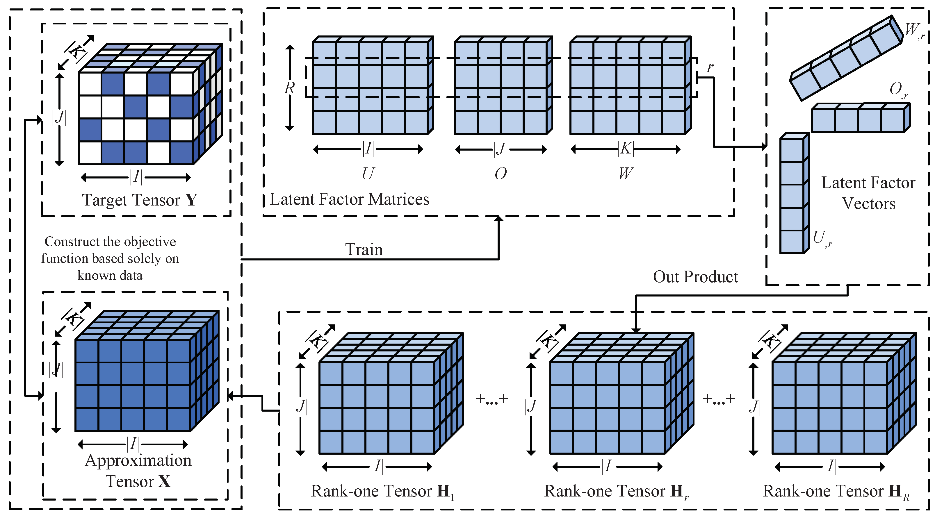
In recent years, tensor factorization models based on CANDECOMP/PARAFAC (CP) decomposition have gained significant attention for their efficiency in large-scale data imputation [22,23,24]. These models utilize multiple low-dimensional matrices to represent latent features, enabling an accurate reconstruction of the original target tensor [25]. Wu et al. proposed the Fused CP (FCP) decomposition model, which integrates priors such as low rank, sparsity, manifold information, and smoothness, and it was successfully applied to image restoration [26]. Luo et al. enhanced non-negative tensor factorization models by introducing bias terms for QoS data imputation [27]. Wu et al. further proposed a PID controlled tensor factorization model for imputing Dynamically Weighted Directed Networks [28]. Ben Said et al. introduced the Spatiotemporal Tensor Completion Model, leveraging enhanced CP decomposition to repair missing values in urban traffic data by incorporating spatial and temporal features [29]. Overall, tensor factorization models demonstrate promising potential and wide applicability in high-dimensional data completion. Zhu et al. developed the Multi-Task Neural Tensor Factorization (MTNTF) model, combining tensor factorization and neural networks to improve the accuracy and efficiency of traffic flow data imputation through multitask learning and attention mechanisms [30]. Jin et al. proposed a Graph-Aware Tensor Factorization Convolutional Network that utilizes Graph Convolutional Networks (GCNs) as the encoder and tensor factorization as the decoder to more effectively represent and complete knowledge graphs [31]. Deng et al. proposed a wireless network traffic prediction model that combines Bayesian Gaussian Tensor Factorization (BGCP) for imputing missing values and RNNs for traffic prediction [32].

Therefore, to address the issue of missing PC data, this study makes the following main contributions:

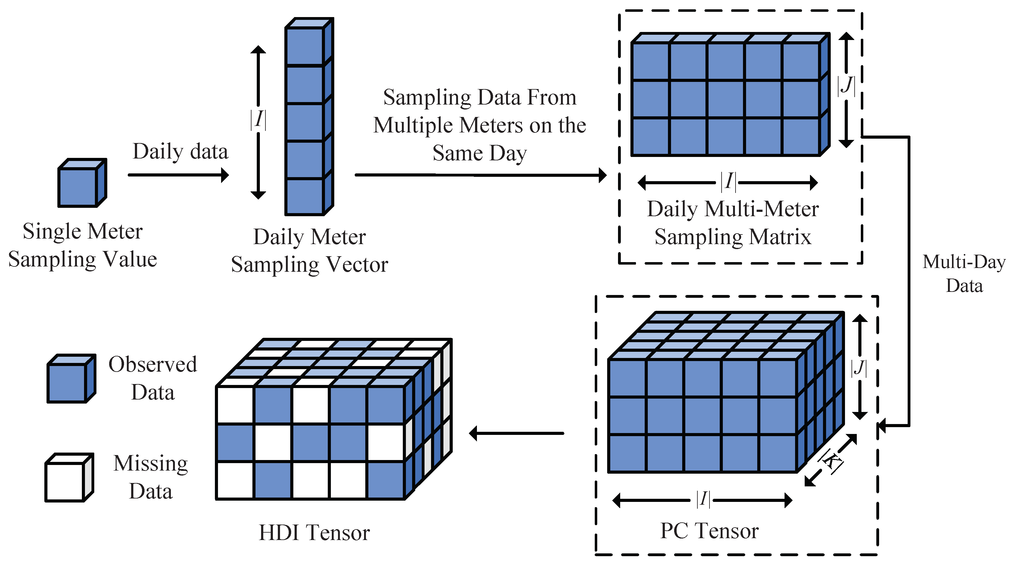
• Third-Order PC Tensor Construction: This study develops a third-order tensor structure that preserves temporal patterns and effectively models inter-appliance relationships. For example, monitoring the PC of 10 devices in a building at a sampling rate of 1 Hz over a 24 h period results in a tensor with dimensions of $10\times 86, 400\times 7$, representing the number of devices, time steps (86,400 s per day), and 7 consecutive days.
• Robust Momentum-Enhanced Non-Negative Tensor Factorization (RMNTF) Model: This study introduces the RMNTF model, enhancing robustness through the integration of adversarial loss and $L_2$ regularization. The sigmoid activation function ensures non-negativity constraints, thereby improving the interpretability of the imputation results. Additionally, momentum-based optimization methods accelerate the optimization process, significantly reducing convergence time.
• Implementation and Performance Evaluation: This study completes detailed implementation and performance evaluations of the RMNTF algorithm on two publicly available PC datasets. The results demonstrate the model’s ability to provide high-accuracy imputation for missing PC data, outperforming existing methods in handling high-sparsity scenarios.

The structure of this paper is as follows: Section 2 outlines the theoretical foundations; Section 3 describes the proposed model in detail; Section 4 presents the experimental results and evaluates the model’s performance; and, finally, Section 5 summarizes the advantages of the RMNTF model in PC data imputation, discusses its key findings and model limitations, and suggests potential directions for future research.

2. Fundamentals

2.1. Symbol Appointment

The symbols adopted in this paper are summarized in

Table 1. Adopted symbols and their descriptions.

Symbol	Description
$I,J,K$	Three entity sets
$\mathbf{Y}$	Third-order target tensor
$\mathbf{H}$	The r-th rank-one tensor
${\mathbf{H}}_{\mathbf{r}}$	The r-th rank-one tensor summed to form $\mathbf{X}$
$\mathbf{X}$	Approximation to $\mathbf{Y}$
$\tilde{\mathbf{Y}}$	The tensor obtained by perturbing $\mathbf{Y}$
$y_{ijk},$$h_{ijk},$$h_{\left(r\right)ijk}$,$x_{ijk}$	Single entry of $\mathbf{Y},$ $\mathbf{H}$, ${\mathbf{H}}_{\mathbf{r}}$, and $\mathbf{X}$
${\tilde{y}}_{ijk}$	Single entry of $\tilde{\mathbf{Y}}$
R	Latent feature dimension or the number of rank-one tensors
$U,O,W$	Latent factor matrices
$U_{,r},O_{,r},W_{,r}$	The r-th latent factor vectors in $U,O$, and W
$u_{ir},o_{jr},w_{kr}$	Single entry of $U,O$, and W
$Q_{\left(U\right)},Q_{\left(O\right)},Q_{\left(W\right)}$	Decision parameter matrices
$Q_{\left(U\right)ir},Q_{\left(O\right)jr},Q_{\left(W\right)kr}$	Single entry of $Q_{\left(U\right)},Q_{\left(O\right)},$ and $Q_{\left(W\right)}$
$M_{\left(U\right)ir},M_{\left(O\right)jr},M_{\left(W\right)kr}$	The historical momentum of $Q_{\left(U\right)ir},Q_{\left(O\right)jr},Q_{\left(W\right)kr}$
$\delta$	Perturbation magnitude
${\lambda }_a,{\lambda }_b$	$L_2$ and adversarial regularization coefficients
$\eta$	Learning rate
$\gamma$	Momentum coefficient
∘	Outer product of two vectors
$\left|·\right|$	Number of elements in the set
${∥·∥}_F$	Tensor’s frobenius norm
$\Lambda ,\Gamma$	The observed and missing entries of tensor $\mathbf{Y}$
$\Phi ,\Psi ,\Omega$	Training, validation, and testing subsets from $\Lambda$
t	Iteration counts

.

2.2. PC Data Tensorization

This study employs two publicly available PC datasets for an empirical analysis: iAWE [33] and REDD [34]. The iAWE dataset encompasses energy usage data from multiple households, capturing device-level usage patterns. In contrast, the REDD dataset provides high-frequency consumption data from several residential buildings, emphasizing the differentiation of energy usage patterns across various devices. However, both datasets exhibit inherent missing value issues, including both continuous and random missing data, which pose significant challenges to the accuracy of data analyses. This issue is particularly critical in high-temporal-resolution scenarios, where the effective handling of missing data is essential.

In the analysis of PC data, intrinsic correlations may exist among different dimensions—namely, date, time samples, and devices. By representing the data as a low-rank tensor, high-dimensional data can be approximated using a limited number of latent patterns, thereby facilitating data compression and imputation.

• Date Dimension: Captures energy consumption variations across different dates, revealing usage patterns on weekdays versus weekends and identifying periodic trends over time [35].
• Time Sample Dimension: Encapsulates consumption characteristics at various times of the day, highlighting differences between morning and evening usage patterns and uncovering periodic consumption behaviors for specific devices [36].
• Device Dimension: Represents the array of devices within the monitored environment, enabling an analysis of inter-device correlations. For example, the usage of certain devices (e.g., computers) may be highly correlated with the operation of others (e.g., air conditioners) [37].

To construct the tensor, this study selects three consecutive weeks of PC data from the iAWE and REDD datasets. The datasets contain a proportion of missing values, and only a subset of the known data is utilized in the tensor construction to simulate a high sparsity rate. The resulting tensor comprises three dimensions: device, time sample, and date. Specifically, the device dimension includes 12 m from the iAWE dataset and 18 m from the REDD dataset; the time sample dimension corresponds to 86,400 sampling points per day, indicating a one-second sampling rate; and the date dimension spans three weeks (21 days) of data. This multidimensional representation effectively captures inter-device correlations and periodic data characteristics, enabling the application of advanced tensor decomposition techniques to uncover latent patterns and relationships. Detailed information about the tensor, including the number of meters, data sampling time range, number of time samples, and other specific attributes for each dataset, is provided in

Table 2. Tensorization details.

Attributes	D1 (iAWE)	D2 (REDD)
Sampling Rate	1 Hz	1 Hz
Days	21	21
Samples per Day	86,400	86,400
Meter Quantity	12	18
Tensor Dimensions	$21\times 86, 400\times 12$	$21\times 86, 400\times 18$
Entries	1,448,417	1,579,227
Density	6.65%	4.80%

.

Definition 1.

(HDI PC tensor): Consider three sets I, J, and K, representing time steps, appliances, and days, respectively. Let $\mathbf{Y}$ denote a tensor of dimensions $\left|I\right|\times \left|J\right|\times \left|K\right|$. Each $y_{ijk}$ element in $\mathbf{Y}$ represents the PC of appliance $j\in J$ at time $i\in I$ on day $k\in K$. The $\mathbf{Y}$ tensor is divided into two parts: known data Λ and missing or unknown data Γ. When the amount of known data is much smaller than that of unknown data, i.e., $|\Lambda |\ll |\Gamma |$, and the tensor has more than two dimensions, the $\mathbf{Y}$ tensor is referred to as an HDI tensor. Figure 1 illustrates the process of modeling PC data as this tensor.

To better understand the structure of $\mathbf{Y}$, three types of slices can be considered:

• Horizontal slice: Fixing $k\in K$, a horizontal slice $\mathbf{Y}(:,:,k)$ represents the PC of all appliances across all time steps on a specific day.
• Vertical slice: Fixing $j\in J$, a vertical slice $\mathbf{Y}(:,j,:)$ represents the PC of a specific appliance across all time steps and days.
• Frontal slice: Fixing $i\in I$, a frontal slice $\mathbf{Y}(i,:,:)$ represents the PC of all appliances across all days at a specific time step.

2.3. TF for Missing PC Data Imputation

Definition 2.

(Rank-one tensor): A three-dimensional tensor $\mathbf{H}$ of size $\left|I\right|\times \left|J\right|\times \left|K\right|$ is defined as a rank-one tensor if each element $h_{ijk}$ can be expressed as the product of three scalars:

$$\begin{array}{c}\hfill h_{ijk}=a_i{b}_j{c}_k,\end{array}$$

(1)

where $a_i$, $b_j$, and $c_k$ are elements of the vectors a, b, and c, respectively, with lengths $\left|I\right|$, $\left|J\right|$, and $\left|K\right|$. In this case, $\mathbf{H}$ can be represented as the outer product of the three vectors:

$$\begin{array}{c}\hfill \mathbf{H}=a\circ b\circ c.\end{array}$$

(2)

Definition 3.

(Tensor Factorization (TF)): In this paper, TF is constructed based on CP decomposition (CPD), approximating the target tensor $\mathbf{Y}$ as $\mathbf{X}$, which is the sum of R rank-one tensors, where R is the estimated rank of $\mathbf{X}$. As illustrated in Figure 2, TF approximates $\mathbf{Y}$ using latent factor matrices (LFs) to construct a rank-R tensor $\mathbf{X}$.

Thus, the approximation tensor $\mathbf{X}$ can be expressed as

$$\begin{array}{c}\hfill {\displaystyle \mathbf{X}=\sum _{r=1}^R{\mathbf{H}}_r,}\end{array}$$

(3)

where each ${\mathbf{H}}_r$ is a rank-one tensor, which is represented by the outer product of the r-th column vectors of the LFs $U^{\left|I\right|\times R}$, $O^{\left|J\right|\times R}$, and $W^{\left|K\right|\times R}$ as follows:

$$\begin{array}{c}\hfill {\mathbf{H}}_r=U_{,r}\circ O_{,r}\circ W_{,r}.\end{array}$$

(4)

By Definitions 2 and 3, each entry $x_{ijk}$ in $\mathbf{X}$ can be written as

$$x_{ijk}=\sum _{r=1}^R{h}_{\left(r\right)ijk}=\sum _{r=1}^R{u}_{ir}{o}_{jr}{w}_{kr},$$

(5)

where $u_{ir}$, $o_{jr}$, and $w_{kr}$ are the elements of the latent factor vectors $U_{,r}$, $O_{,r}$, and $W_{,r}$, respectively. Note that determining the rank R is an NP-hard problem, so R is typically predefined to simplify computation.

To quantify the difference between $\mathbf{Y}$ and $\mathbf{X}$, an objective function $\epsilon$ is formulated based on the Euclidean distance. Given that $\mathbf{Y}$ contains only a limited set of known entries $\Lambda$, the objective function is defined as

$${\displaystyle \epsilon =\frac{1}{2}\sum _{y_{ijk}\in \Lambda }{\left(y_{ijk}-x_{ijk}\right)}^2}$$

(6)

To accurately capture the non-negativity of PC data, this study incorporates non-negativity constraints on the LFs within the tensor factorization model. Specifically, (5) is substituted into (6), and non-negativity constraints are added to the objective function, thereby transforming (6) into

$$\begin{array}{c}{\displaystyle \epsilon =\frac{1}{2}\sum _{y_{ijk}\in \Lambda }{\left(y_{ijk}-\sum _{r=1}^R{u}_{ir}{o}_{jr}{w}_{kr}\right)}^2,}\hfill \\ \mathrm{s}.\mathrm{t}.\forall i\in I,j\in J,k\in K,r\in \{1,2,3,\dots ,R\},u_{ir}\ge 0,o_{jr}\ge 0,w_{kr}\ge 0.\hfill \end{array}$$

(7)

To address the imbalance in the distribution of known entries in $\mathbf{Y}$, $L_2$ regularization is introduced (as suggested in [38,39,40]) to prevent overfitting by increasing the penalty on outliers, thereby enhancing the model’s generalization ability. Consequently, the objective function $\epsilon$ is updated as

$$\begin{array}{c}{\displaystyle \epsilon =\frac{1}{2}\sum _{y_{ijk}\in {\Lambda }_a}\left({\left(y_{ijk}-\sum _{r=1}^R{u}_{ir}{o}_{jr}{w}_{kr}\right)}^2+\lambda \sum _{r=1}^R\left(u_{ir}^2+o_{jr}^2+w_{kr}^2\right)\right),}\hfill \\ \mathrm{s}.\mathrm{t}.\forall i\in I,j\in J,k\in K,r\in \{1,2,3,\dots ,R\},u_{ir}\ge 0,o_{jr}\ge 0,w_{kr}\ge 0.\hfill \end{array}$$

(8)

3. RMNTF Model

3.1. Decoupling Non-Negativity Constraints in Tensor Factorization

In this paper, three decision parameter matrices (DPs) are introduced for the LFs U, O, and W, denoted as $Q_{\left(U\right)}^{\left|I\right|\times R}$, $Q_{\left(O\right)}^{\left|J\right|\times R}$, and $Q_{\left(W\right)}^{\left|K\right|\times R}$, respectively. By incorporating DPs, the model decouples the optimization process from the non-negativity constraints, enabling more efficient learning while maintaining flexibility in the optimization of the LFs.

The LFs are generated through a mapping function f applied to the elements of the DPs, defined as

$$\begin{array}{cc}\hfill & u_{ir}=f\left(Q_{\left(U\right)ir}\right),o_{jr}=f\left(Q_{\left(O\right)jr}\right),w_{kr}=f\left(Q_{\left(W\right)kr}\right),\hfill \\ \hfill & \mathrm{s}.\mathrm{t}.\forall i\in I, j\in J, k\in K, r\in \{1,2,\dots ,R\},\hfill \end{array}$$

(9)

where $Q_{{\left(U\right)}_{ir}}$, $Q_{{\left(O\right)}_{jr}}$, and $Q_{{\left(W\right)}_{kr}}$ are elements of the DPs $Q_{\left(U\right)}$, $Q_{\left(O\right)}$, and $Q_{\left(W\right)}$, respectively. Element-wise mapping ensures that the generated LFs automatically satisfy the non-negativity constraints.

To ensure non-negativity, the mapping function f, based on [41], must satisfy the following conditions:

$$\begin{array}{c}\hfill \forall x\in \mathbb{R}:\left\{\begin{array}{cc}f\left(x\right)\ge 0,\hfill & \left(\mathrm{Non-negativity}\right)\hfill \\ \exists x=f^{-1}\left(y\right),\hfill & \left(\mathrm{Invertibility}\right)\hfill \\ f^{\prime }\left(x\right)\ne 0,\hfill & (\mathrm{Non-zero} \mathrm{derivative})\hfill \end{array}\right.\end{array}$$

(10)

Based on these conditions, the sigmoid function is selected as the mapping function, defined as

$$\begin{array}{c}\hfill f\left(x\right)=\frac{1}{1+e^{-x}},\hspace{1em}{f}^{\prime }\left(x\right)=f\left(x\right)·(1-f\left(x\right)).\end{array}$$

(11)

The derivative $f^{\prime }\left(x\right)$ approaches zero as $\left|x\right|\to \infty$ but never equals zero, thus satisfying all necessary conditions.

The flexibility of the sigmoid function allows the DPs $Q_{\left(U\right)}$, $Q_{\left(O\right)}$, and $Q_{\left(W\right)}$ to take values freely in the real number domain while ensuring that the LFs are non-negative. This characteristic guarantees that the reconstructed tensor $\mathbf{X}$ remains non-negative, consistent with the physical significance of PC data. Furthermore, nonlinear mapping enhances the model’s ability to capture complex relationships and patterns, thereby improving overall representation performance.

As a result, the objective function $\epsilon$, which appears in (8), is reformulated as

$$\begin{array}{cc}\hfill & {\displaystyle \epsilon =\frac{1}{2}\sum _{y_{ijk}\in \Lambda }\left({\left(y_{ijk}-x_{ijk}\right)}^2+\lambda \sum _{r=1}^R\left(f{\left(Q_{\left(U\right)ir}\right)}^2+f{\left(Q_{\left(O\right)jr}\right)}^2+f{\left(Q_{\left(W\right)kr}\right)}^2\right)\right),}\hfill \\ \hfill & \mathrm{s}.\mathrm{t}.\forall i\in I, j\in J, k\in K, r\in \{1,2,\dots ,R\}.\hfill \end{array}$$

(12)

3.2. Adversarial Loss Regularization for Enhanced Robustness

To enhance the robustness and generalization ability of the model, an adversarial loss regularization term is introduced into the objective function. By adding carefully designed perturbations to the true values, the model simulates worst-case input variations, forcing it to learn features that are robust to these disturbances. This approach improves the model’s performance in diverse and noisy environments [42,43].

The first step is to generate adversarial samples by maximizing the following objective function, which aims to create perturbations by maximizing the error between the observed and reconstructed samples:

$$\max \mathcal{L}=\max \frac{1}{2}\sum _{y_{ijk}\in \Lambda }{(y_{ijk}-x_{ijk})}^2.$$

(13)

Maximizing this objective function generates perturbations that increase the error between the perturbed samples and the model’s predictions.

For each observed value $y_{ijk}$, perturbations are generated using the Fast Gradient Sign Method (FGSM) [42]. The FGSM computes the gradient of the objective function with respect to the observed value to determine the direction and magnitude of the perturbation. Specifically, the perturbed value ${\tilde{y}}_{ijk}$ is given by

$${\tilde{y}}_{ijk}=y_{ijk}+\delta ·\mathrm{sign}\left(\frac{\partial \mathcal{L}}{\partial y_{ijk}}\right)=y_{ijk}+\delta ·\mathrm{sign}\left(e_{ijk}\right),$$

(14)

where $\delta$ is a hyperparameter controlling the magnitude of the perturbation, and $e_{ijk}=y_{ijk}-x_{ijk}$ is the error between the observed value and the reconstructed value, indicating deviation from the model’s reconstruction.

The sign function $\mathrm{sign}\left(e_{ijk}\right)$ plays a crucial role in perturbation generation, determining the direction and magnitude of the perturbation. Specifically, the sign function operates as follows:

• If $e_{ijk}>0$, i.e., $y_{ijk}>x_{ijk}$, then $\mathrm{sign}\left(e_{ijk}\right)=1$, meaning that the perturbation is added to $y_{ijk}$ (i.e., $y_{ijk}$ is increased).
• If $e_{ijk}<0$, i.e., $y_{ijk}<x_{ijk}$, then $\mathrm{sign}\left(e_{ijk}\right)=-1$, meaning that the perturbation is subtracted from $y_{ijk}$ (i.e., $y_{ijk}$ is decreased).
• If $e_{ijk}=0$, then no perturbation is applied.

This method ensures that the perturbation is applied in the direction of the model’s prediction error, maximizing the model’s ability to adapt to worst-case input scenarios.

Based on the perturbed reconstructed value ${\tilde{y}}_{ijk}$, the adversarial regularization term ${\mathcal{L}}_{\mathrm{adv}}$ is defined to incorporate the perturbation’s effect into the model’s training. This regularization term measures the difference between the perturbed sample and the reconstructed data, and it is given by

$${\mathcal{L}}_{\mathrm{adv}}=\frac{1}{2}\sum _{y_{ijk}\in \Lambda }{\left({\tilde{y}}_{ijk}-x_{ijk}\right)}^2=\frac{1}{2}\sum _{y_{ijk}\in \Lambda }{\left(e_{ijk}+\delta ·\mathrm{sign}\left(e_{ijk}\right)\right)}^2.$$

(15)

The purpose of this regularization term is to dynamically adjust the instance error through perturbations, thereby enhancing the model’s sensitivity to disturbances.

By adding the regularization term (15) into the objective function (12), the adversarially regularized objective function $\tilde{\epsilon }$ becomes

$$\tilde{\epsilon }=\epsilon +{\lambda }_b{\mathcal{L}}_{\mathrm{adv}},$$

(16)

where ${\lambda }_b$ is a hyperparameter controlling the weight of the adversarial regularization term, balancing the influence of the original error and the adversarial loss. By minimizing $\tilde{\epsilon }$, the model not only reduces the prediction error on the original data but also strengthens its robustness to perturbed data. Figure 3 presents the procedure for perturbing the $\mathbf{Y}$ tensor to generate the perturbed tensor $\tilde{\mathbf{Y}}$.

3.3. Stochastic Gradient Descent (SGD)-Based Tensor Factorization Model

According to [27,28,44], SGD reduces computational complexity by iteratively optimizing the gradient of individual samples (or mini-batches), making it particularly suitable for high-dimensional and large-scale tensor factorization. Additionally, its simplicity and ease of implementation further enhance its applicability. Therefore, this study employs SGD to minimize the objective function in (16), with the update rules specified as follows:

$$\begin{array}{cc}\hfill \arg min \tilde{\epsilon } (Q_{\left(U\right)},& Q_{\left(O\right)},Q_{\left(W\right)})\stackrel{\mathrm{SGD}}{⟶}\forall i\in I,j\in J,k\in K,r\in \{1,\dots ,R\},\hfill \\ \hfill & Q_{\left(U\right)ir}^{t+1}\leftarrow Q_{\left(U\right)ir}^t-\eta \frac{\partial {\tilde{\epsilon }}_{ijk}^t}{\partial Q_{\left(U\right)ir}^t};\hfill \\ \hfill & Q_{\left(O\right)jr}^{t+1}\leftarrow Q_{\left(O\right)jr}^t-\eta \frac{\partial {\tilde{\epsilon }}_{ijk}^t}{\partial Q_{\left(O\right)jr}^t};\hfill \\ \hfill & Q_{\left(W\right)kr}^{t+1}\leftarrow Q_{\left(W\right)kr}^t-\eta \frac{\partial {\tilde{\epsilon }}_{ijk}^t}{\partial Q_{\left(W\right)kr}^t},\hfill \end{array}$$

(17)

where ${\tilde{\epsilon }}_{ijk}$ is the element-wise error term in the objective function $\tilde{\epsilon }$, representing the contribution of the error at position $(i,j,k)$ to the entire objective function.

The detailed computation of the gradients of ${\tilde{\epsilon }}_{ijk}$ with respect to the DPs $Q_{\left(U\right)}$, $Q_{\left(O\right)}$, and $Q_{\left(W\right)}$ in (17) is as follows:

$$\begin{array}{cc}\hfill \frac{\partial {\tilde{\epsilon }}_{ijk}^t}{\partial Q_{\left(U\right)ir}^t}= & f^{\prime }\left(Q_{\left(U\right)ir}^t\right)\left({\lambda }_{a}f\left(Q_{\left(U\right)ir}^t\right)-\left(e_{ijk}^t+{\lambda }_b\left({\tilde{y}}_{ijk}-x_{ijk}\right)\right)f\left(Q_{\left(O\right)jr}^t\right)f\left(Q_{\left(W\right)kr}^t\right)\right),\hfill \\ \hfill \frac{\partial {\tilde{\epsilon }}_{ijk}^t}{\partial Q_{\left(O\right)jr}^t}= & f^{\prime }\left(Q_{\left(O\right)jr}^t\right)\left({\lambda }_{a}f\left(Q_{\left(O\right)jr}^t\right)-\left(e_{ijk}^t+{\lambda }_b\left({\tilde{y}}_{ijk}-x_{ijk}\right)\right)f\left(Q_{\left(U\right)ir}^t\right)f\left(Q_{\left(W\right)kr}^t\right)\right),\hfill \\ \hfill \frac{\partial {\tilde{\epsilon }}_{ijk}^t}{\partial Q_{\left(W\right)kr}^t}= & f^{\prime }\left(Q_{\left(W\right)kr}^t\right)\left({\lambda }_{a}f\left(Q_{\left(W\right)kr}^t\right)-\left(e_{ijk}^t+{\lambda }_b\left({\tilde{y}}_{ijk}-x_{ijk}\right)\right)f\left(Q_{\left(U\right)ir}^t\right)f\left(Q_{\left(O\right)jr}^t\right)\right).\hfill \end{array}$$

(18)

3.4. Incorporating Momentum in TF

The Momentum Method is a technique used to accelerate the optimization of gradient descent [45,46]. By introducing the concept of “momentum” in parameter updates, it reduces oscillations during training and speeds up convergence. The core idea of the Momentum Method is to apply an exponentially weighted moving average of past gradients to the current gradient update. This means that, when updating parameters, it not only considers the current gradient but also accumulates information from previous gradients, thus accelerating in steep directions and reducing oscillations in winding paths.

The update formulas of the Momentum Method are as follows:

$$\begin{array}{cc}\hfill & M^0=0;\hfill \\ \hfill & M^t=\gamma M^{t-1}+\eta \nabla \left({\theta }^{t-1}\right);\hfill \\ \hfill & {\theta }^t={\theta }^{t-1}-M^t,\hfill \end{array}$$

(19)

where ${\theta }^t$ represents the parameter value at the t-th iteration, and $M^t$ represents the updated “momentum”, which is the weighted sum of the current gradient and the historical gradients.

To accelerate convergence in solving the tensor factorization model, the SGD algorithm is improved. By combining (17) and (19), the update rule for the decision parameter matrix $Q_{\left(U\right)ir}$ based on the Momentum Method is given as

$$\begin{array}{cc}\hfill & M_{Q_{\left(U\right)ir}}^0=0,\hfill \\ \hfill & M_{Q_{\left(U\right)ir}}^{t+1}=\gamma M_{Q_{\left(U\right)ir}}^t+\eta \frac{\partial {\tilde{\epsilon }}_{ijk}^t}{\partial Q_{\left(U\right)ir}},\hfill \\ \hfill & Q_{\left(U\right)ir}^{t+1}=Q_{\left(U\right)ir}^t-M_{Q_{\left(U\right)ir}}^{t+1}.\hfill \end{array}$$

(20)

Since the momentum-based update rules of $Q_{{\left(S\right)}_{jr}}$ and $Q_{{\left(W\right)}_{kr}}$ are similar to those of $Q_{{\left(U\right)}_{ir}}$, they are not presented here. In this paper, three auxiliary matrices, $M_{Q_{\left(U\right)}}^{\left|I\right|\times R}$, $M_{Q_{\left(O\right)}}^{\left|J\right|\times R}$, and $M_{Q_{\left(W\right)}}^{\left|K\right|\times R}$, are used to record the historical momenta of the DPs $Q_{\left(U\right)}$, $Q_{\left(O\right)}$, and $Q_{\left(W\right)}$. Based on (17) and (20), the detailed update rules of the DPs are as follows:

$$\left\{\begin{array}{c}{M}_{Q_{\left(U\right)ir}}^{t+1}=\gamma M_{Q_{\left(U\right)ir}}^t+\eta \frac{\partial {\tilde{\epsilon }}_{ijk}^t}{\partial Q_{\left(U\right)ir}^t},Q_{\left(U\right)ir}^{t+1}=Q_{\left(U\right)ir}^t-M_{Q_{\left(U\right)ir}}^{t+1}; \hfill \\ M_{Q_{\left(O\right)jr}}^{t+1}=\gamma M_{Q_{\left(O\right)jr}}^t+\eta \frac{\partial {\tilde{\epsilon }}_{ijk}^t}{\partial Q_{\left(O\right)jr}^t},Q_{\left(O\right)jr}^{t+1}=Q_{\left(O\right)jr}^t-M_{Q_{\left(O\right)jr}}^{t+1}; \hfill \\ M_{Q_{\left(W\right)kr}}^{t+1}=\gamma M_{Q_{\left(W\right)kr}}^t+\eta \frac{\partial {\tilde{\epsilon }}_{ijk}^t}{\partial Q_{\left(W\right)kr}^t}, Q_{\left(W\right)kr}^{t+1}=Q_{\left(W\right)kr}^t-M_{Q_{\left(W\right)kr}}^{t+1}.\hfill \end{array}\right.$$

(21)

The RMNTF model is fully presented as described above.

3.5. Algorithm Design and Analysis

Building on the above, this paper presents Algorithm 1, which aims to optimize model performance by updating the DPs. This process involves calculating historical momentum and applying dynamic error perturbations. The computational complexity is

$$\begin{array}{cc}\hfill C& =\Theta \left(\left(\left|I\right|+\left|J\right|+\left|K\right|\right)\times 2R+t\times \left|\Lambda \right|\times 2R\right)\hfill \\ \hfill & \approx \Theta (t\times \left|\Lambda \right|\times R).\hfill \end{array}$$

(22)

Algorithm 1 RMNTF
	Input:  $I,J,K,R,\Lambda ,\eta ,{\lambda }_a,{\lambda }_b,\delta$
	output: $f\left(Q_{\left(U\right)}\right),f\left(Q_{\left(O\right)}\right),f\left(Q_{\left(W\right)}\right)$
	Operation		Cost
	1:	Initialize $Q_{\left(U\right)}^{\left|I\right|\times R},Q_{\left(O\right)}^{\left|J\right|\times R},Q_{\left(W\right)}^{\left|K\right|\times R}$ with random numbers	$\Theta \left(\left(\left|I\right|+\left|J\right|+\left|K\right|\right)\times R\right)$
	2:	Initialize $M_{\left(U\right)}^{\left|I\right|\times R},M_{\left(O\right)}^{\left|J\right|\times R},M_{\left(W\right)}^{\left|K\right|\times R}$ with zeros	$\Theta \left(\left(\left|I\right|+\left|J\right|+\left|K\right|\right)\times R\right)$
	3:	Initialize $t=1,T=max\_iteration\_count$	$\Theta \left(1\right)$
	4:	while $t<T$ $\mathbf{and} \mathbf{not}$ converge $\mathbf{do}$	$\times \mathrm{t}$
	5:	for $y_{ijk}$ $in$ $\Lambda$ do	$\times \Theta \left(\left|\Lambda \right|\right)$
	6:	$x_{ijk}={\sum }_{r=1}^{R}f\left(Q_{{\left(U\right)}_{ir}}\right)·f\left(Q_{{\left(O\right)}_{jr}}\right)·f\left(Q_{{\left(W\right)}_{kr}}\right)$	$\Theta \left(R\right)$
	7:	Compute ${\tilde{y}}_{ijk}$ using (14)	$\Theta \left(1\right)$
	8:	for $r=1$ to R do	$\times R$
	9:	$M_{Q_{\left(U\right)ir}}=\gamma M_{Q_{\left(U\right)ir}}+\eta \frac{\partial {\tilde{\epsilon }}_{ijk}}{\partial Q_{\left(U\right)ir}}$	$\Theta \left(1\right)$
	10:	$M_{Q_{\left(O\right)jr}}=\gamma M_{Q_{\left(O\right)jr}}+\eta \frac{\partial {\tilde{\epsilon }}_{ijk}}{\partial Q_{\left(O\right)jr}}$	$\Theta \left(1\right)$
	11:	$M_{Q_{\left(W\right)kr}}=\gamma M_{Q_{\left(W\right)kr}}+\eta \frac{\partial {\tilde{\epsilon }}_{ijk}}{\partial Q_{\left(W\right)kr}}$	$\Theta \left(1\right)$
	12:	$Q_{\left(U\right)ir}=Q_{\left(U\right)ir}-M_{Q_{\left(U\right)ir}}$	$\Theta \left(1\right)$
	13:	$Q_{\left(O\right)jr}=Q_{\left(O\right)jr}-M_{Q_{\left(O\right)jr}}$	$\Theta \left(1\right)$
	14:	$Q_{\left(W\right)kr}=Q_{\left(W\right)kr}-M_{Q_{\left(W\right)kr}}$	$\Theta \left(1\right)$
	15:	end for	−
	16:	end for	−
	17:	end while	−

In practical scenarios (as shown in Table 2), $\left(\right|\Lambda \left|\right)\gg \max \left\{\right|I|,|J|,|K\left|\right\}$. Thus, lower-order terms and coefficients are omitted to derive (22). Furthermore, given that n and R are both positive, the computational complexity of RMNTF can be inferred to be linear with respect to the number of known elements $|\Lambda |$.

The storage complexity is primarily determined by three factors: (1) the DPs $Q_{\left(U\right)},$$Q_{\left(O\right)},$ and $Q_{\left(W\right)}$ and their corresponding LFs $U,$ O, and W; (2) the auxiliary matrices $M_{\left(U\right)},M_{\left(O\right)},M_{\left(W\right)}$ used to store the historical momentum information of the DPs; and (3) the entries in the set $|\Lambda |$, along with their corresponding reconstructed values. Therefore, the storage complexity of the model is given by

$$\begin{array}{cc}\hfill S& =\Theta \left(\right(\left|I\right|+\left|J\right|+\left|K\right|)\times 3R+2\times |\Lambda \left|\right)\hfill \\ \hfill & \approx \left(\left|I\right|+\left|J\right|+\left|K\right|\right)\times R+|\Lambda |.\hfill \end{array}$$

(23)

In (23), the storage complexity of the RMNTF model primarily depends on the number of known tensor entries and the dimensionality of latent factors, both of which exhibit a linear relationship.

4. Experimental Results and Discussion

4.1. Experimental Setup and Evaluation

4.1.1. Dataset Normalization

Excessively large PC values may lead to numerical instability or overflow during optimization. To ensure stable and robust updates, the datasets are normalized by rescaling the values to the range [0, 10] using the following formula:

$$y=10\times \frac{y-y_{\min }}{y_{\max }-y_{\min }}.$$

(24)

4.1.2. Traning Setting

All experiments were conducted on a system with an Intel Core i7-10700 processor (2.9 GHz) and 16 GB of RAM, running Python 3.11.5 as the primary programming environment. For the comparison models, those using neural networks were accelerated by GPU support from a cloud platform, specifically an NVIDIA 2080 Ti (11GB VRAM).

To ensure the reliability of the experimental results, the dataset was divided into non-overlapping training ($\Phi$), validation ($\Psi$), and testing ($\Omega$) sets, as detailed in

Table 3. Training and testing data splits for D1 and D2.

Dataset No.	D1		D2
	D1.1	D1.2	D2.1	D2.2
Training–Testing	60%:20%	30%:40%	60%:20%	30%:40%
Training data	869,050	434,525	947,536	473,768
Testing data	289,683	579,366	315,845	631,691

. The model optimized the LFs by minimizing the objective function on the training set, with convergence assessed based on validation metrics. Finally, the learned LFs were evaluated on the test set to measure model performance.

To further guarantee fairness and objectivity, the following experimental protocols were implemented:

• To reduce random errors and enhance reliability, each experiment was repeated 20 times on each dataset.
• Training was terminated under either of the following conditions: the change in the validation error over three consecutive iterations was less than 1 × 10⁻⁶ (indicating convergence), or the maximum number of iterations reached 500.
• The latent factor dimension R was fixed at 10 across all TF models to balance computational efficiency and ensure comparability.
• All model hyperparameters were optimized using a grid search to achieve optimal performance.

4.1.3. Evaluation Metrics

The performance of PC data imputation reflects the model’s ability to capture inherent patterns in incomplete tensors and accurately fit the data structure and feature distribution. To comprehensively evaluate the model’s performance, two metrics are employed: the Root Mean Square Error (RMSE) and the Mean Absolute Error (MAE) [47,48,49]. The RMSE measures the deviation between predicted and true values, with sensitivity to larger errors, making it suitable for extreme data scenarios. In contrast, the MAE calculates the average absolute differences, providing a more intuitive assessment of overall error levels. Together, these metrics offer a complementary evaluation of the model’s imputation capability, defined as follows:

$$\begin{array}{c}\hfill \mathrm{RMSE}=\sqrt{\frac{{\sum }_{y_{ijk}\in \mathcal{D}}{\left(y_{ijk}-x_{ijk}\right)}^2}{\left|\mathcal{D}\right|}}; \mathrm{MAE}=\frac{{\sum }_{y_{ijk}\in \mathcal{D}}\left|y_{ijk}-x_{ijk}\right|}{\left|\mathcal{D}\right|},\end{array}$$

(25)

where $\mathcal{D}$ may be either $\Psi$ or $\Omega$.

4.2. Comparison of TF and NTF Model Performance

To investigate the impact of the sigmoid activation function on model performance, a comparison is made between the TF and NTF models. Figure 4 illustrates the performance of both models across different datasets. The following conclusions can be drawn from the results:

• Due to the effect of the sigmoid function, the TF and NTF models exhibit different sensitivities to the learning rate $\eta$. However, for the $\eta$, both models show a decrease in the iteration count, accompanied by a slight increase in imputation errors. For instance, in Figure 4a–d, on the D1.1 dataset, as the $\eta$ increases from $1\times {10}^{-4}$ to $6\times {10}^{-4}$, TF’s RMSE increases from 0.1279 to 0.1295, with the iteration count decreasing from 327 to 87; MAE rises from 0.0617 to 0.0636, and the iteration count drops from 465 to 96. Similarly, on the D2.1 dataset, as the $\eta$ increases from 0.1 to 0.6, NTF’s RMSE increases from 0.2258 to 0.2274, with the iteration count decreasing from 109 to 21; the MAE increases from 0.0418 to 0.0426, and the iteration count drops from 132 to 28.
• NTF achieves lower imputation errors than TF. As shown in Figure 4a,c, on the D1.2 dataset, when the learning rate $\eta$ is set to $1\times {10}^{-4}$, TF’s RMSE and MAE are 0.1395 and 0.0678, respectively. When $\eta$ is set to 0.1, NTF’s RMSE and MAE are 0.1356 and 0.0616, showing reductions of 2.80% and 9.14%, respectively $\left(\left(Valu{e}_{high}-valu{e}_{low}\right)/Valu{e}_{high}\right)$. On the D2.2 dataset, TF’s RMSE and MAE are 0.2346 and 0.0440, respectively. When $\eta$ is set to 0.1, NTF’s RMSE and MAE are 0.2262 and 0.0424, showing improvements of 3.58% and 3.64%, respectively. Similar results are observed for other learning rates and datasets.

4.3. Hyperparameter Sensitivity Analysis

As discussed in Section 4.2, the choice of the hyperparameter $\eta$ is critical for model performance. Additionally, as outlined in Section 3, the model’s performance is also influenced by the $L_2$ regularization coefficient ${\lambda }_a$, adversarial regularization coefficient ${\lambda }_b$, perturbation magnitude $\delta$, and momentum coefficient $\gamma$. This section, therefore, provides an experimental analysis of the impact of these parameters on model performance.

4.3.1. Impacts of ${\lambda }_a$ and ${\lambda }_b$

With the other hyperparameters fixed, Figure 5a,b shows the effects of increasing ${\lambda }_a$ from $5\times {10}^{-5}$ to $5\times {10}^{-3}$ on the model imputation error and iteration count. Figure 5c,d illustrates the impact of increasing ${\lambda }_b$ from $1\times {10}^{-4}$ to $1\times {10}^0$. Based on these results, the following conclusions can be drawn:

• The selection of ${\lambda }_a$ is critical to model performance. A smaller ${\lambda }_a$ can result in overfitting, while a larger ${\lambda }_a$ can degrade the model’s ability to fit the data. As shown in Figure 5a, for D1.1, as ${\lambda }_a$ increases from $5\times {10}^{-5}$ to $5\times {10}^{-4}$, the RMSE decreases from 0.12546 to 0.1239. However, when ${\lambda }_a$ is further increased to $5\times {10}^{-3}$, the RMSE rises to 0.1317. Similarly, for D2.1, as ${\lambda }_a$ increases from $5\times {10}^{-5}$ to $1\times {10}^{-4}$ and then to $5\times {10}^{-3}$, the MAE decreases from 0.0437 to 0.0428 and then increases to 0.0468. Additionally, the number of iterations increases with ${\lambda }_a$. As illustrated in Figure 5b, in D1.2, the iteration count for the MAE rises from 138 to 500 as ${\lambda }_a$ increases from $5\times {10}^{-5}$ to $5\times {10}^{-3}$. In D2.2, for the RMSE, the iteration count increases from 55 to 121 as ${\lambda }_a$ increases from $5\times {10}^{-5}$ to $5\times {10}^{-3}$.
• The appropriate selection of ${\lambda }_b$ is critical for reducing overfitting and enhancing the robustness of the model, thereby achieving lower imputation errors. As illustrated in Figure 5c, for dataset D1.1, when ${\lambda }_b=1\times {10}^{-2}$, the RMSE and MAE reach their minimum values of 0.1237 and 0.0551, respectively. Similarly, for D2.1, when ${\lambda }_b=1\times {10}^{-1}$, the RMSE and MAE are minimized to 0.02262 and 0.0396, respectively. The iteration count of the model increases with ${\lambda }_b$. As shown in Figure 5d, when ${\lambda }_b$ increases from $1\times {10}^{-4}$ to $1\times {10}^0$, the iteration counts for the RMSE and MAE decrease from 120 to 72 and from 209 to 97 in D1.2, respectively. In D2.2, the iteration counts for the RMSE and MAE decrease from 48 to 21 and from 37 to 18, respectively.

4.3.2. Impacts of $\gamma$ and $\delta$

As shown in Figure 6, changes in $\gamma$ and $\delta$ significantly affect the model’s imputation error and the number of iterations. The key observations are as follows:

• $\gamma$ controls the accumulation of historical gradients. As $\gamma$ increases, the number of iterations rises, while the imputation error shows no significant change. As shown in Figure 6a,b, for the D1.1 dataset, as $\gamma$ increases from 0.1 to 0.6, the RMSE changes from 0.1236 to 0.1242, and the MAE changes from 0.05784 to 0.0580. The iteration counts for the RMSE and MAE decrease from 78 to 34 and from 166 to 66, respectively. In the D2.1 dataset, the RMSE changes from 0.2268 to 0.2280, and the MAE changes from 0.04062 to 0.04046. The iteration counts for the RMSE and MAE decrease from 42 to 22 and from 33 to 14, respectively. This indicates that, although increasing $\gamma$ accelerates convergence, it has little impact on the imputation error.
• The noise perturbation $\delta$ controls the model’s robustness by simulating uncertainties or fluctuations in the data. An appropriate value of $\delta$ enhances the model’s stability and adaptability when facing such uncertainties. As shown in Figure 6c, on the D1.2 dataset, when $\delta$ is set to 0.05 and 0.1, the RMSE and MAE reach their optimal values of 0.1241 and 0.0551. On the D2.2 dataset, the RMSE is minimized at $\delta =0.05$ with a value of 0.0227, while the MAE decreases from 0.0445 to 0.0380 as $\delta$ increases from 0.005 to 1. As $\delta$ increases, the model’s iteration count decreases. As shown in Figure 6d, on the D1.1 dataset, the iteration counts for the RMSE and MAE decrease from 105 and 189 to 58 and 67, respectively, as $\delta$ increases from 0.005 to 1. On the D2.1 dataset, the iteration counts for the RMSE and MAE decrease from 52 and 32 to 28 and 15, respectively.

4.4. Comparison with State-of-the-Art Models

4.4.1. Models for Comparison

The seven state-of-the-art models used for comparison are described in detail below:

• M1: Time-SVD++ [50], a model based on two factor matrices that incorporates time-dependent biases and dynamic feature vectors to effectively capture temporal dynamics during factorization.
• M2: PLFT [28], a TF model integrating PID control principles with SGD to enhance optimization and convergence. It employs linear bias vectors for data fitting and $L_2$ regularization to prevent overfitting and improve stability.
• M3: NeuLFT [44], a nonlinear TF model for HDI tensors. It integrates rank-one tensors as hidden neurons in a single-layer feedback network, uses an adaptive backward propagation (ABP) learning scheme with Momentum-SGD and Particle Swarm Optimization (PSO), applies a sigmoid activation function for nonlinear modeling, and incorporates linear bias tensors with $L_2$ regularization.
• M4: HaLRTC [9], a low-rank tensor completion model that extends NNM to tensors using a novel tensor trace norm definition. It employs the Alternating Direction Method of Multipliers (ADMM) for efficient optimization, enabling accurate estimations of missing values in high-dimensional data.
• M5: RTC-ASVD [51], a robust tensor completion model leveraging approximate singular value decomposition (SVD) with fast QR decomposition and tensor $\gamma$-nuclear norm regularization. It combines discrete Fourier transform (DFT) techniques and ADMM for optimization, effectively addressing missing and corrupted data in high-dimensional tensors.
• M6: NT-DPTC [52], a tensor completion model using dimension-preserved (DP) tensor decomposition to maintain traffic data structure. It decomposes the tensor into three latent factor tensors, applies a sigmoid function for non-negativity, and uses AdamW for efficient optimization and convergence.
• M7: LSTM [15], a specialized RNN model with memory cells and gating mechanisms to capture long-term dependencies in time series data, particularly suited for tasks like multi-step forecasting and imputation.
• M8: RMNTF, the model proposed in this paper.

4.4.2. Theoretical Complexity Comparison

In this section, the theoretical time and space complexities of the proposed RMNTF (M8) model are compared with those of three baseline models: TF, HaLRTC (M4), and NT-DPTC (M6). The TF model, as the most basic tensor factorization method, serves as a baseline for comparison; M4 is a classical low-rank tensor completion model based on matrix NNM and is widely used for tensor completion tasks; M6 employs DP decomposition and trains solely on observed data, sharing similarities with M8 in terms of tensor factorization and optimization strategies. By comparing the theoretical complexities of these three models, the theoretical advantages of M8 can be highlighted.

Table 4. Computational and storage complexity of different models.

Model	Computational Complexity	Storage Complexity
TF	$\Theta \left(t\times R\times \left|\Lambda \right|\right)$	$\Theta \left((\left|I\right|+\left|J\right|+\left|K\right|)\times R+\left|\Lambda \right|\right)$
M4	$\Theta \left(t\times \left(\left|I\right|\times \left|J\right|\times \left|K\right|\times \min \left(\left|I\right|,\left|J\right|,\left|K\right|\right)\right)\right)$	$\Theta \left(\left|I\right|\times \left|J\right|\times \left|K\right|\right)$
M6	$\Theta \left(t\times \left|\Lambda \right|\times (\left|K\right|\times \left|I\right|\times R+\left|K\right|\times \left|J\right|\times R+\left|I\right|\times \left|J\right|)\right)$	$\Theta \left((\left|K\right|\times \left|I\right|\times R+\left|K\right|\times R\times \left|J\right|+\left|I\right|\times \left|J\right|)+\left|\Lambda \right|\right)$
M8	$\Theta \left(t\times R\times \left|\Lambda \right|\right)$	$\Theta \left((\left|I\right|+\left|J\right|+\left|K\right|)\times R+\left|\Lambda \right|\right)$

presents the time and space complexities of the models, and the following conclusions can be drawn:

In the case of the HDI tensor, M8 demonstrates strong competitiveness in terms of complexity compared to the other models. As shown in Table 4, M8 and TF exhibit identical time and space complexities, indicating that M8 does not introduce significant additional complexity compared to TF. M4, due to its optimization process requiring matrix singular value decomposition and the reconstruction of the complete tensor, exhibits significantly higher time and space complexities. When the tensor is extremely sparse, i.e., $\left|I\right|\times \left|J\right|\times \left|K\right|\gg |\Lambda |$, the complexity of M4 becomes even more pronounced. Compared to M6, M8 exhibits superior time and space complexities, making it more efficient in handling large-scale sparse data.

4.4.3. Comparison Results

Table 5. Performance comparison of models across datasets using the MAE and RMSE metrics.

Dataset	Metric	M1	M2	M3	M4	M5	M6	M7	M8
D1.1	RMSE	$0.{1288}_{\pm 6\times {10}^{-4}}$	$0.{1271}_{\pm 3\times {10}^{-3}}$	$0.{1268}_{\pm 5\times {10}^{-4}}$	$0.{1560}_{\pm 0}$	$0.{1964}_{\pm 3\times {10}^{-6}}$	$0.{1468}_{\pm 4\times {10}^{-6}}$	$0.{1403}_{\pm 1\times {10}^{-6}}$	$\mathbf{0}.{\mathbf{1247}}_{\pm \mathbf{6}\times {\mathbf{10}}^{-\mathbf{4}}}$
	MAE	$0.{0664}_{\pm 5\times {10}^{-4}}$	$0.{0637}_{\pm 2\times {10}^{-3}}$	$0.{0587}_{\pm 2\times {10}^{-3}}$	$0.{0769}_{\pm 0}$	$0.{0914}_{\pm 2\times {10}^{-6}}$	$0.{0697}_{\pm 6\times {10}^{-6}}$	$0.{0596}_{\pm 1\times {10}^{-6}}$	$\mathbf{0}.{\mathbf{0568}}_{\pm \mathbf{1}\times {\mathbf{10}}^{-\mathbf{3}}}$
D1.2	RMSE	$0.{1387}_{\pm 4\times {10}^{-4}}$	$0.{1390}_{\pm 4\times {10}^{-3}}$	$0.{1376}_{\pm 4\times {10}^{-4}}$	$0.{1951}_{\pm 0}$	$0.{2074}_{\pm 3\times {10}^{-6}}$	$0.{1643}_{\pm 5\times {10}^{-6}}$	$0.{1426}_{\pm 1\times {10}^{-6}}$	$\mathbf{0}.{\mathbf{1336}}_{\pm \mathbf{8}\times {\mathbf{10}}^{-\mathbf{4}}}$
	MAE	$0.{0711}_{\pm 3\times {10}^{-4}}$	$0.{0697}_{\pm 2\times {10}^{-3}}$	$0.{0676}_{\pm 2\times {10}^{-3}}$	$0.{0963}_{\pm 0}$	$0.{1023}_{\pm 3\times {10}^{-6}}$	$0.{0818}_{\pm 4\times {10}^{-6}}$	$0.{0687}_{\pm 2\times {10}^{-6}}$	$\mathbf{0}.{\mathbf{0633}}_{\pm \mathbf{4}\times {\mathbf{10}}^{-\mathbf{4}}}$
D2.1	RMSE	$0.{2336}_{\pm 3\times {10}^{-4}}$	$0.{2296}_{\pm 2\times {10}^{-3}}$	$0.{2316}_{\pm 6\times {10}^{-4}}$	$0.{2557}_{\pm 0}$	$0.{2560}_{\pm 8\times {10}^{-6}}$	$0.{2338}_{\pm 1\times {10}^{-5}}$	$0.{2541}_{\pm 1\times {10}^{-7}}$	$\mathbf{0}.{\mathbf{2262}}_{\pm \mathbf{1}\times {\mathbf{10}}^{-\mathbf{3}}}$
	MAE	$0.{0433}_{\pm 5\times {10}^{-4}}$	$0.{0422}_{\pm 1\times {10}^{-3}}$	$0.{0456}_{\pm 8\times {10}^{-4}}$	$0.{0452}_{\pm 0}$	$0.{0482}_{\pm 1\times {10}^{-5}}$	$0.{0544}_{\pm 9\times {10}^{-6}}$	$0.{0623}_{\pm 5\times {10}^{-6}}$	$\mathbf{0}.{\mathbf{0376}}_{\pm \mathbf{2}\times {\mathbf{10}}^{-\mathbf{4}}}$
D2.2	RMSE	$0.{2291}_{\pm 3\times {10}^{-4}}$	$0.{2295}_{\pm 1\times {10}^{-3}}$	$0.{2307}_{\pm 5\times {10}^{-4}}$	$0.{2545}_{\pm 0}$	$0.{2559}_{\pm 7\times {10}^{-6}}$	$0.{2386}_{\pm 5\times {10}^{-6}}$	$0.{2489}_{\pm 3\times {10}^{-7}}$	$\mathbf{0}.{\mathbf{2263}}_{\pm \mathbf{3}\times {\mathbf{10}}^{-\mathbf{3}}}$
	MAE	$0.{0442}_{\pm 2\times {10}^{-4}}$	$0.{0431}_{\pm 8\times {10}^{-4}}$	$0.{0469}_{\pm 3\times {10}^{-4}}$	$0.{0473}_{\pm 0}$	$0.{0477}_{\pm 6\times {10}^{-6}}$	$0.{0635}_{\pm 1\times {10}^{-5}}$	$0.{0646}_{\pm 1\times {10}^{-6}}$	$\mathbf{0}.{\mathbf{0378}}_{\pm \mathbf{4}\times {\mathbf{10}}^{-\mathbf{4}}}$

The bold values represent the best performance for each metric. The “±” values represent the standard deviation.

presents the imputation errors of the various models across datasets, reflecting their performance under optimal parameters.

Table 6. Time consumption of models across datasets (seconds).

Dataset	Metric	M1	M2	M3	M4	M5	M6	M7	M8
D1.1	RMSE	$32.{36}_{\pm 2.27}$	$54.{61}_{\pm 3.03}$	$335.{89}_{\pm 32.35}$	$336.{36}_{\pm 1.20}$	$87.{62}_{\pm 2.47}$	$147.{03}_{\pm 1.40}$	$229.{24}_{\pm 1.49}$	$\mathbf{31}.{\mathbf{44}}_{\pm \mathbf{2}.\mathbf{6}}$
	MAE	$\mathbf{39}.{\mathbf{47}}_{\pm \mathbf{2}.\mathbf{55}}$	$62.{63}_{\pm 3.38}$	$423.{74}_{\pm 38.67}$	$1054.{46}_{\pm 1.01}$	$72.{45}_{\pm 2.41}$	$167.{64}_{\pm 2.07}$	$231.{41}_{\pm 1.33}$	$42.{63}_{\pm 1.98}$
D1.2	RMSE	$35.{62}_{\pm 2.37}$	$56.{52}_{\pm 4.52}$	$305.{36}_{\pm 29.13}$	$334.{64}_{\pm 1.26}$	$81.{54}_{\pm 1.96}$	$118.{91}_{\pm 1.14}$	$230.{44}_{\pm 1.10}$	$\mathbf{32}.{\mathbf{26}}_{\pm \mathbf{1}.\mathbf{88}}$
	MAE	$\mathbf{35}.{\mathbf{41}}_{\pm \mathbf{2}.\mathbf{81}}$	$82.{43}_{\pm 4.32}$	$403.{25}_{\pm 27.66}$	$1046.{95}_{\pm 1.96}$	$67.{53}_{\pm 2.57}$	$127.{60}_{\pm 2.41}$	$236.{21}_{\pm 1.79}$	$37.{37}_{\pm 1.54}$
D2.1	RMSE	$13.{89}_{\pm 0.65}$	$24.{32}_{\pm 1.20}$	$178.{65}_{\pm 16.81}$	$99.{32}_{\pm 0.96}$	$36.{80}_{\pm 1.66}$	$28.{18}_{\pm 2.04}$	$235.{74}_{\pm 1.74}$	$\mathbf{11}.{\mathbf{28}}_{\pm \mathbf{0}.\mathbf{68}}$
	MAE	$14.{23}_{\pm 0.74}$	$31.{86}_{\pm 2.03}$	$203.{36}_{\pm 17.61}$	$107.{74}_{\pm 1.34}$	$41.{56}_{\pm 1.68}$	$36.{20}_{\pm 1.44}$	$235.{41}_{\pm 2.04}$	$\mathbf{11}.{\mathbf{56}}_{\pm \mathbf{0}.\mathbf{73}}$
D2.2	RMSE	$9.{06}_{\pm 0.61}$	$21.{74}_{\pm 1.14}$	$170.{63}_{\pm 14.69}$	$102.{32}_{\pm 0.64}$	$30.{74}_{\pm 1.25}$	$20.{98}_{\pm 1.09}$	$232.{56}_{\pm 1.41}$	$\mathbf{7}.{\mathbf{30}}_{\pm \mathbf{0}.\mathbf{57}}$
	MAE	$9.{45}_{\pm 0.64}$	$24.{31}_{\pm 1.56}$	$190.{57}_{\pm 16.54}$	$111.{74}_{\pm 1.54}$	$43.{20}_{\pm 2.26}$	$22.{36}_{\pm 1.12}$	$237.{69}_{\pm 1.77}$	$\mathbf{7}.{\mathbf{96}}_{\pm \mathbf{0}.\mathbf{89}}$

The bold values represent the best performance for each metric. The “±” values represent the standard deviation.

complements this by comparing the time consumption of each model, providing additional context on computational efficiency. From these results, the following findings can be observed:

• M8 achieves lower imputation errors across all datasets, outperforming all other comparable models. As shown in Table 5, on the D1.1 dataset, M8 has an RMSE of 0.1247 and an MAE of 0.0568, which are 1.92% and 10.83% lower than those of the second-best model, M2, with RMSE and MAE values of 0.1271 and 0.0637, respectively. On the D2.1 dataset, M8 has an RMSE of 0.2262 and an MAE of 0.0376, which are 1.48% and 10.40% lower than those of M2, with RMSE and MAE values of 0.2296 and 0.0422, respectively. On the D1.2 dataset, M8 reduces the RMSE by an average of 14.59% and the MAE by 17.37% compared to all other models. On the D2.2 dataset, M8 reduces the RMSE by an average of 5.31% and the MAE by 25.53% compared to all other models. Overall, M8 demonstrates superior imputation accuracy across all datasets, further solidifying its potential for practical data imputation tasks.
• M8 demonstrates significant efficiency advantages over the other models. As shown in Table 6, on the D2.1 dataset, the computation times of the RMSE and MAE with M8 are 11.28 and 11.56, respectively, lower than those of the second-best model M1, which takes 13.89 and 14.23, representing reductions of 18.79% and 18.76%, respectively. On the D2.2 dataset, M8 further reduces the RMSE and MAE computation times to 7.30 and 7.96, a decrease of 19.43% and 15.77% compared to those of M2. On the D1.1 dataset, M8 achieves an average reduction of 66.56% and 60.77% in computation times for the RMSE and MAE, respectively, compared to the other models. On the D1.2 dataset, M8 also shows superior performance, with average reductions of 64.34% and 63.46% for the RMSE and MAE computation times.

To assess the statistical significance of the performance differences between the models, the Wilcoxon signed-rank test is applied. This non-parametric paired comparison method evaluates three key metrics: ${\mathrm{R}}^{+}$ (the sum of ranks for positive differences), ${\mathrm{R}}^{-}$ (the sum of ranks for negative differences), and the p-value. A larger R+ value indicates better performance, while the p-value determines statistical significance. When the p-value is below the significance level (typically 0.05), the difference is considered statistically significant.

Table 7. Statistical results of the Wilcoxon signed-rank test for the RMSE and MAE in Table 5.

Comparison	R+	R−	p-Value
M8 vs. M1	36	0	0.0078
M8 vs. M2	36	0	0.0078
M8 vs. M3	36	0	0.0078
M8 vs. M4	36	0	0.0078
M8 vs. M5	36	0	0.0078
M8 vs. M6	36	0	0.0078
M8 vs. M7	36	0	0.0078

and

Table 8. Statistical results of the Wilcoxon signed-rank test for time consumption in Table 6.

Comparison	R+	R−	p-Value
M8 vs. M1	26	10	0.3828
M8 vs. M2	36	0	0.0078
M8 vs. M3	36	0	0.0078
M8 vs. M4	36	0	0.0078
M8 vs. M5	36	0	0.0078
M8 vs. M6	36	0	0.0078
M8 vs. M7	36	0	0.0078

summarize the Wilcoxon test results based on Table 5 and Table 6, where the RMSE and MAE are used as evaluation metrics across four datasets. Thus, each model corresponds to eight comparison cases. The following conclusions can be drawn from these statistical results:

M8 demonstrates significant improvements in both accuracy and efficiency compared to the other models. As shown in Table 7 and Table 8, M8 consistently achieves high ${\mathrm{R}}^{+}$ values and low p-values. Moreover, M8 outperforms all other models in nearly all test scenarios, with the ${\mathrm{R}}^{-}$ values being zero in 13 out of 14 comparisons, as indicated in the tables. The only exception is in the comparison of computational efficiency between M8 and M1, where M8’s computation time slightly exceeds that of M1 when using the MAE metric on the D1.1 and D1.2 datasets, as recorded in Table 6.

4.5. Summary

The experimental results demonstrate that the RMNTF model excels in two key areas: (a) efficient computational performance and (b) accurate and stable imputation capability, particularly for handling high-missing-rate PC data. These strengths establish RMNTF as a reliable solution for PC data imputation tasks.

5. Discussion

The findings of this study provide valuable insights into PC data analyses, particularly in the context of high-dimensional and incomplete data. Our proposed RMNTF model demonstrates significant improvements in both accuracy and computational efficiency over existing methods. This section discusses the results in relation to those of previous studies, the working hypotheses, and their broader implications, and it suggests potential directions for future research.

Our results support the working hypothesis that integrating adversarial loss regularization and $L_2$ regularization enhances the robustness of tensor factorization models in the presence of incomplete data. RMNTF’s superior performance, evidenced by lower RMSE and MAE values across all datasets, highlights the effectiveness of these regularization techniques. This is consistent with prior studies, which emphasize the benefits of regularization in improving generalization and stability in machine learning models [53,54]. Another key contribution of our model is the enforcement of non-negativity constraints via the sigmoid function, ensuring that imputed values are physically meaningful and interpretable. This aligns with the inherent characteristics of PC data, which cannot be negative, and represents a significant advancement over models that do not incorporate such constraints. The momentum-based optimization approach in RMNTF has proven to be an effective tool for accelerating convergence, reducing the computational burden compared to that of traditional tensor factorization methods. This is especially relevant for large-scale applications, where time and resource efficiency are critical.

The implications of our findings go beyond PC data analyses. RMNTF’s ability to accurately handle high-dimensional and incomplete data makes it applicable across various domains, including finance, healthcare, and social network analyses [55,56,57], where such data characteristics are common. The model’s robustness and interpretability make it a valuable tool for decision-making in these fields.

Despite the promising results demonstrated by RMNTF, several limitations must be addressed in future work:

• Computational Resource Requirements: While RMNTF performs well in terms of computational efficiency, its resource demands remain high when processing large-scale datasets. In resource-constrained environments, such as embedded systems or mobile devices, scalability and parallelization are crucial. Future research should focus on adapting RMNTF for distributed computing and parallel frameworks to improve efficiency in large-scale applications [58,59].
• Complexity of Parameter Selection: The model’s performance is highly sensitive to hyperparameters (e.g., regularization and momentum coefficients). Selecting appropriate parameters often requires extensive experimentation and tuning, which adds complexity. Future work should explore smarter hyperparameter optimization methods, such as Bayesian optimization or metaheuristic algorithms, to automate the selection of optimal parameters and enhance both usability and efficiency [60,61].
• Real-World Validation: Although RMNTF has been tested on public datasets, these may not fully capture the complexities of real industrial environments. Validating the model in real-world settings is essential to assess its effectiveness, robustness, and stability, especially in environments with higher noise and data uncertainty. Future research should focus on applying the model to industrial applications and conducting field validation to evaluate its performance in real-time data processing [62,63].
• Limitations of Data Sources: The datasets used in this study are primarily sourced from publicly available PC datasets, which may introduce biases and limit the model’s generalizability. Future research should consider more diverse data sources, including different building types, regions, and devices, to improve the model’s adaptability and generalization capability [64].
• Data Quality Limitations: Although the datasets have been cleaned and preprocessed, noise and outliers may still persist, affecting model accuracy. Future work should adopt more advanced noise filtering and outlier detection methods to enhance data quality and ensure stable model training and prediction [65,66].

In conclusion, the RMNTF model represents a significant advancement in tensor factorization for handling missing PC data. Its effectiveness, robustness, and efficiency position it as a leading solution for data imputation tasks. Future research will further refine and expand the model’s capabilities, ensuring its continued relevance and impact in the era of big data.

References

1. Zabin, R.; Haque, K.F.; Abdelgawad, A. PredXGBR: A Machine Learning Framework for Short-Term Electrical Load Prediction. Electronics 2024, 13, 4521. [Google Scholar] [CrossRef]
2. Dong, A.; Lee, S.K. The Study of Scheduling Optimization for Multi-Microgrid Systems Based on an Improved Differential Algorithm. Electronics 2024, 13, 4517. [Google Scholar] [CrossRef]
3. Lin, R.; Ye, Z.; Zhao, Y. OPEC: Daily load data analysis based on optimized evolutionary clustering. Energies 2019, 12, 2668. [Google Scholar] [CrossRef]
4. Li, Z.H.; Cui, J.X.; Chen, H.Y.; Lu, H.P.; Zhou, F.; Rocha, P.R.F.; Yang, C.Y. Research Progress of All-Fiber Optic Current Transformers in Novel Power Systems: A Review. Microw. Opt. Technol. Lett. 2025, 67, e70061. [Google Scholar] [CrossRef]
5. Ramadan, R.; Huang, Q.; Zalhaf, A.S.; Bamisile, O.; Li, J.; Mansour, D.E.A.; Lin, X.; Yehia, D.M. Energy Management in Residential Microgrid Based on Non-Intrusive Load Monitoring and Internet of Things. Smart Cities 2024, 7, 1907–1935. [Google Scholar] [CrossRef]
6. Basu, S.; Matteson, D.S. A survey of estimation methods for sparse high-dimensional time series models. arXiv 2021, arXiv:2107.14754. [Google Scholar] [CrossRef]
7. Beretta, L.; Santaniello, A. Nearest neighbor imputation algorithms: A critical evaluation. BMC Med. Inform. Decis. Mak. 2016, 16, 197–208. [Google Scholar] [CrossRef]
8. Athey, S.; Bayati, M.; Doudchenko, N.; Imbens, G.; Khosravi, K. Matrix completion methods for causal panel data models. J. Am. Stat. Assoc. 2021, 116, 1716–1730. [Google Scholar] [CrossRef]
9. Liu, J.; Musialski, P.; Wonka, P.; Ye, J. Tensor completion for estimating missing values in visual data. IEEE Trans. Pattern Anal. Mach. Intell. 2012, 35, 208–220. [Google Scholar] [CrossRef]
10. Zhang, Z.; Aeron, S. Exact tensor completion using t-SVD. IEEE Trans. Signal Process. 2016, 65, 1511–1526. [Google Scholar] [CrossRef]
11. Ullah, I.; Ahmad, R.; Kim, D. A prediction mechanism of energy consumption in residential buildings using hidden markov model. Energies 2018, 11, 358. [Google Scholar] [CrossRef]
12. Maruotti, A. Mixed hidden markov models for longitudinal data: An overview. Int. Stat. Rev. 2011, 79, 427–454. [Google Scholar] [CrossRef]
13. Duarte, O.; Duarte, J.E.; Rosero-Garcia, J. Data Imputation in Electricity Consumption Profiles through Shape Modeling with Autoencoders. Mathematics 2024, 12, 3004. [Google Scholar] [CrossRef]
14. Kim, J.C.; Chung, K. Recurrent neural network-based multimodal deep learning for estimating missing values in healthcare. Appl. Sci. 2022, 12, 7477. [Google Scholar] [CrossRef]
15. Yuan, H.; Xu, G.; Yao, Z.; Jia, J.; Zhang, Y. Imputation of missing data in time series for air pollutants using long short-term memory recurrent neural networks. In Proceedings of the 2018 ACM International Joint Conference and 2018 International Symposium on Pervasive and Ubiquitous Computing and Wearable Computers, Singapore, 8–12 October 2018; pp. 1293–1300. [Google Scholar] [CrossRef]
16. Lee, D.; Kim, J.; Moon, W.J.; Ye, J.C. CollaGAN: Collaborative GAN for missing image data imputation. In Proceedings of the IEEE/CVF Conference on Computer Vision and Pattern Recognition, Long Beach, CA, USA, 15–20 June 2019; pp. 2487–2496. Available online: https://openaccess.thecvf.com/content_CVPR_2019/html/Lee_CollaGAN_Collaborative_GAN_for_Missing_Image_Data_Imputation_CVPR_2019_paper.html (accessed on 16 January 2025).
17. Wong, L.Z.; Chen, H.; Lin, S.; Chen, D.C. Imputing missing values in sensor networks using sparse data representations. In Proceedings of the 17th ACM International Conference on Modeling, Analysis and Simulation of Wireless and Mobile Systems, Miami Beach, FL, USA, 21–25 November 2014; pp. 227–230. [Google Scholar] [CrossRef]
18. Song, S.; Sun, Y.; Zhang, A.; Chen, L.; Wang, J. Enriching data imputation under similarity rule constraints. IEEE Trans. Knowl. Data Eng. 2018, 32, 275–287. [Google Scholar] [CrossRef]
19. Breve, B.; Caruccio, L.; Deufemia, V.; Polese, G. RENUVER: A Missing Value Imputation Algorithm based on Relaxed Functional Dependencies. In Proceedings of the EDBT 2022, Edinburgh, UK, 29 March–1 April 2022; pp. 1–52. [Google Scholar]
20. Mohan, K.; Pearl, J. Graphical Models for Recovering Probabilistic and Causal Queries from Missing Data. Adv. Neural Inf. Process. Syst. 2014, 27, 1520–1528. [Google Scholar]
21. Qiao, L.; Cui, Y.; Jia, Z.; Xiao, K.; Su, H. Missing well logs prediction based on hybrid kernel extreme learning machine optimized by Bayesian optimization. Appl. Sci. 2022, 12, 7838. [Google Scholar] [CrossRef]
22. Acar, E.; Dunlavy, D.M.; Kolda, T.G.; Mørup, M. Scalable tensor factorizations for incomplete data. Chemom. Intell. Lab. Syst. 2011, 106, 41–56. [Google Scholar] [CrossRef]
23. Song, Q.; Ge, H.; Caverlee, J.; Hu, X. Tensor completion algorithms in big data analytics. ACM Trans. Knowl. Discov. Data (TKDD) 2019, 13, 1–48. [Google Scholar] [CrossRef]
24. Mørup, M. Applications of tensor (multiway array) factorizations and decompositions in data mining. Wiley Interdiscip. Rev. Data Min. Knowl. Discov. 2011, 1, 24–40. [Google Scholar] [CrossRef]
25. Kolda, T.G.; Bader, B.W. Tensor decompositions and applications. SIAM Rev. 2009, 51, 455–500. [Google Scholar] [CrossRef]
26. Wu, Y.; Tan, H.; Li, Y.; Zhang, J.; Chen, X. A fused CP factorization method for incomplete tensors. IEEE Trans. Neural Netw. Learn. Syst. 2018, 30, 751–764. [Google Scholar] [CrossRef] [PubMed]
27. Luo, X.; Wu, H.; Yuan, H.; Zhou, M. Temporal pattern-aware QoS prediction via biased non-negative latent factorization of tensors. IEEE Trans. Cybern. 2019, 50, 1798–1809. [Google Scholar] [CrossRef] [PubMed]
28. Wu, H.; Luo, X.; Zhou, M.; Rawa, M.J.; Sedraoui, K.; Albeshri, A. A PID-incorporated latent factorization of tensors approach to dynamically weighted directed network analysis. IEEE/CAA J. Autom. Sin. 2021, 9, 533–546. [Google Scholar] [CrossRef]
29. Zhu, Y.; Wang, J.; Wang, J.; He, Z. Multitask neural tensor factorization for road traffic speed-volume correlation pattern learning and joint imputation. IEEE Trans. Intell. Transp. Syst. 2022, 23, 24550–24560. [Google Scholar] [CrossRef]
30. Said, A.B.; Erradi, A. Spatiotemporal tensor completion for improved urban traffic imputation. IEEE Trans. Intell. Transp. Syst. 2021, 23, 6836–6849. [Google Scholar] [CrossRef]
31. Jin, Y.; Yang, L. Graph-aware tensor factorization convolutional network for knowledge graph completion. Int. J. Mach. Learn. Cybern. 2024, 15, 1755–1766. [Google Scholar] [CrossRef]
32. Deng, T.; Wan, M.; Shi, K.; Zhu, L.; Wang, X.; Jiang, X. Short term prediction of wireless traffic based on tensor decomposition and recurrent neural network. SN Appl. Sci. 2021, 3, 779. [Google Scholar] [CrossRef]
33. Batra, N.; Gulati, M.; Singh, A.; Srivastava, M.B. It’s Different: Insights into home energy consumption in India. In Proceedings of the 5th ACM Workshop on Embedded Systems For Energy-Efficient Buildings, Roma, Italy, 11–15 November 2013; pp. 1–8. [Google Scholar] [CrossRef]
34. Kolter, J.Z.; Johnson, M.J. REDD: A public data set for energy disaggregation research. In Proceedings of the Workshop on Data Mining Applications in Sustainability (SIGKDD), San Diego, CA, USA, 21 August 2011; Volume 25, pp. 59–62. Available online: https://citeseerx.ist.psu.edu/document?repid=rep1&type=pdf&doi=d85a51e2978f4563ee74bf9a09d3219e03799819 (accessed on 16 January 2025).
35. Pickering, E.M.; Hossain, M.A.; French, R.H.; Abramson, A.R. Building electricity consumption: Data analytics of building operations with classical time series decomposition and case based subsetting. Energy Build. 2018, 177, 184–196. [Google Scholar] [CrossRef]
36. Singh, S.; Yassine, A. Big data mining of energy time series for behavioral analytics and energy consumption forecasting. Energies 2018, 11, 452. [Google Scholar] [CrossRef]
37. Wilhelm, S.; Kasbauer, J. Exploiting smart meter power consumption measurements for human activity recognition (HAR) with a motif-detection-based non-intrusive load monitoring (NILM) approach. Sensors 2021, 21, 8036. [Google Scholar] [CrossRef]
38. Ma, H.; Zhou, D.; Liu, C.; Lyu, M.R.; King, I. Recommender systems with social regularization. In Proceedings of the Fourth ACM International Conference on Web Search and Data Mining, Hong Kong, China, 9–12 February 2011. [Google Scholar] [CrossRef]
39. Zhang, W.; Sun, H.; Liu, X.; Guo, X. Temporal QoS-aware web service recommendation via non-negative tensor factorization. In Proceedings of the WWW ‘14: 23rd International World Wide Web Conference, Seoul, Republic of Korea, 7–11 April 2014. [Google Scholar] [CrossRef]
40. Takács, G.; Pilászy, I.; Németh, B.; Tikk, D. Scalable collaborative filtering approaches for large recommender systems. J. Mach. Learn. Res. 2009, 10, 623–656. [Google Scholar]
41. Boyd, S.; Vandenberghe, L. Convex Optimization; Cambridge University Press: Cambridge, UK, 2004. [Google Scholar]
42. Goodfellow, I.J.; Shlens, J.; Szegedy, C. Explaining and harnessing adversarial examples. arXiv 2014, arXiv:1412.6572. [Google Scholar] [CrossRef]
43. Kurakin, A.; Goodfellow, I.J.; Bengio, S. Adversarial examples in the physical world. In Artificial Intelligence Safety and Security; Chapman and Hall/CRC: Boca Raton, FL, USA, 2018; pp. 99–112. [Google Scholar] [CrossRef]
44. Luo, X.; Wu, H.; Li, Z. NeuLFT: A novel approach to nonlinear canonical polyadic decomposition on high-dimensional incomplete tensors. IEEE Trans. Knowl. Data Eng. 2022, 35, 6148–6166. [Google Scholar] [CrossRef]
45. Qian, N. On the momentum term in gradient descent learning algorithms. Neural Netw. 1999, 12, 145–151. [Google Scholar] [CrossRef]
46. Ruder, S. An overview of gradient descent optimization algorithms. arXiv 2016, arXiv:1609.04747. [Google Scholar] [CrossRef]
47. Morup, M.; Dunlavy, D.M.; Acar, E.; Kolda, T.G. Scalable Tensor Factorizations with Missing Data; Technical report; Sandia National Laboratories (SNL): Albuquerque, NM, USA; Livermore, CA, USA, 2010. [Google Scholar]
48. Zhang, F.; Gong, T.; Lee, V.E.; Zhao, G.; Rong, C.; Qu, G. Fast Algorithms to Evaluate Collaborative Filtering Recommender Systems; Elsevier: Amsterdam, The Netherlands, 2016; Volume 96. [Google Scholar] [CrossRef]
49. Bhargava, P.; Phan, T.; Zhou, J.; Lee, J. Who, What, When, and Where: Multi-Dimensional Collaborative Recommendations Using Tensor Factorization on Sparse User-Generated Data. In Proceedings of the 24th International Conference on World Wide Web, Florence, Italy, 18–22 May 2015. [Google Scholar] [CrossRef]
50. Koren, Y. Collaborative filtering with temporal dynamics. Commun. In Proceedings of the KDD09: The 15th ACM SIGKDD International Conference on Knowledge Discovery and Data Mining, Paris, France, 28 June–1 July 2009; pp. 447–456. [Google Scholar] [CrossRef]
51. Wu, F.; Li, C.; Li, Y.; Tang, N. Robust low-rank tensor completion via new regularized model with approximate SVD. Inf. Sci. 2023, 629, 646–666. [Google Scholar] [CrossRef]
52. Chen, H.; Lin, M.; Liu, J.; Yang, H.; Zhang, C.; Xu, Z. NT-DPTC: A non-negative temporal dimension preserved tensor completion model for missing traffic data imputation. Inf. Sci. 2024, 653, 119797. [Google Scholar] [CrossRef]
53. Bousquet, O.; Elisseeff, A. Stability and generalization. J. Mach. Learn. Res. 2002, 2, 499–526. [Google Scholar]
54. Xu, H.; Caramanis, C.; Mannor, S. Robustness and Regularization of Support Vector Machines. J. Mach. Learn. Res. 2009, 10, 1485–1510. [Google Scholar]
55. Tabassum, S.; Pereira, F.S.; Fernandes, S.; Gama, J. Social network analysis: An overview. Wiley Interdiscip. Rev. Data Min. Knowl. Discov. 2018, 8, e1256. [Google Scholar] [CrossRef]
56. Ye, J.; Liu, J. Sparse methods for biomedical data. ACM Sigkdd Explor. Newsl. 2012, 14, 4–15. [Google Scholar] [CrossRef]
57. Sorjamaa, A.; Corona, F.; Miche, Y.; Merlin, P.; Maillet, B.; Séverin, E.; Lendasse, A. Sparse linear combination of SOMs for data imputation: Application to financial database. In Proceedings of the Advances in Self-Organizing Maps: 7th International Workshop, WSOM 2009, St. Augustine, FL, USA, 8–10 June 2009; pp. 290–297. [Google Scholar] [CrossRef]
58. Shin, K.; Sael, L.; Kang, U. Fully scalable methods for distributed tensor factorization. IEEE Trans. Knowl. Data Eng. 2016, 29, 100–113. [Google Scholar] [CrossRef]
59. Choi, J.H.; Vishwanathan, S. DFacTo: Distributed factorization of tensors. Adv. Neural Inf. Process. Syst. 2014, 27, 1296–1304. [Google Scholar]
60. Wu, J.; Chen, X.Y.; Zhang, H.; Xiong, L.D.; Lei, H.; Deng, S.H. Hyperparameter optimization for machine learning models based on Bayesian optimization. J. Electron. Sci. Technol. 2019, 17, 26–40. Available online: https://www.sciencedirect.com/science/article/pii/S1674862X19300047 (accessed on 16 January 2025).
61. Joseph, S.B.; Dada, E.G.; Abidemi, A.; Oyewola, D.O.; Khammas, B.M. Metaheuristic algorithms for PID controller parameters tuning: Review, approaches and open problems. Heliyon 2022, 8, e09399. [Google Scholar] [CrossRef]
62. Sun, B.; Xu, Y.; Gu, W.; Cai, H.; Lu, S.; Mili, L.; Yu, W.; Wu, Z. A Low-Rank Tensor Train Approach for Electric Vehicle Load Data Reconstruction Using Real Industrial Data. IEEE Trans. Smart Grid 2024. [Google Scholar] [CrossRef]
63. Li, H.; Li, K.; An, J.; Li, K. An online and scalable model for generalized sparse nonnegative matrix factorization in industrial applications on multi-GPU. IEEE Trans. Ind. Inform. 2019, 18, 437–447. [Google Scholar] [CrossRef]
64. Xu, X.; Cao, X.; Yu, L. Carbon emissions forecasting based on tensor decomposition with multi-source data fusion. Inf. Sci. 2024, 681, 121235. [Google Scholar] [CrossRef]
65. Liu, H.; Chen, C. Data processing strategies in wind energy forecasting models and applications: A comprehensive review. Appl. Energy 2019, 249, 392–408. [Google Scholar] [CrossRef]
66. Li, Z.h.; Cui, J.x.; Lu, H.p.; Zhou, F.; Diao, Y.l.; Li, Z.x. Prediction model of measurement errors in current transformers based on deep learning. Rev. Sci. Instrum. 2024, 95, 044704. [Google Scholar] [CrossRef] [PubMed]
Figure 1. A three-dimensional tensor representation of PC data.
Electronics 14 00351 g001
Figure 2. Factorizing the target tensor Y .
Electronics 14 00351 g002
Figure 3. Building the perturbed tensor Y ˜ from the observed tensor Y .
Electronics 14 00351 g003
Figure 4. Comparison of TF and NTF models’ performance.
Electronics 14 00351 g004
Figure 5. Impacts of λ a and λ b .
Electronics 14 00351 g005
Figure 6. Impacts of γ and δ .
Electronics 14 00351 g006