
Detecting Defects in Solar Panels Using the YOLO v10 and v11 Algorithms


Abstract
1. Introduction
2. Datasets
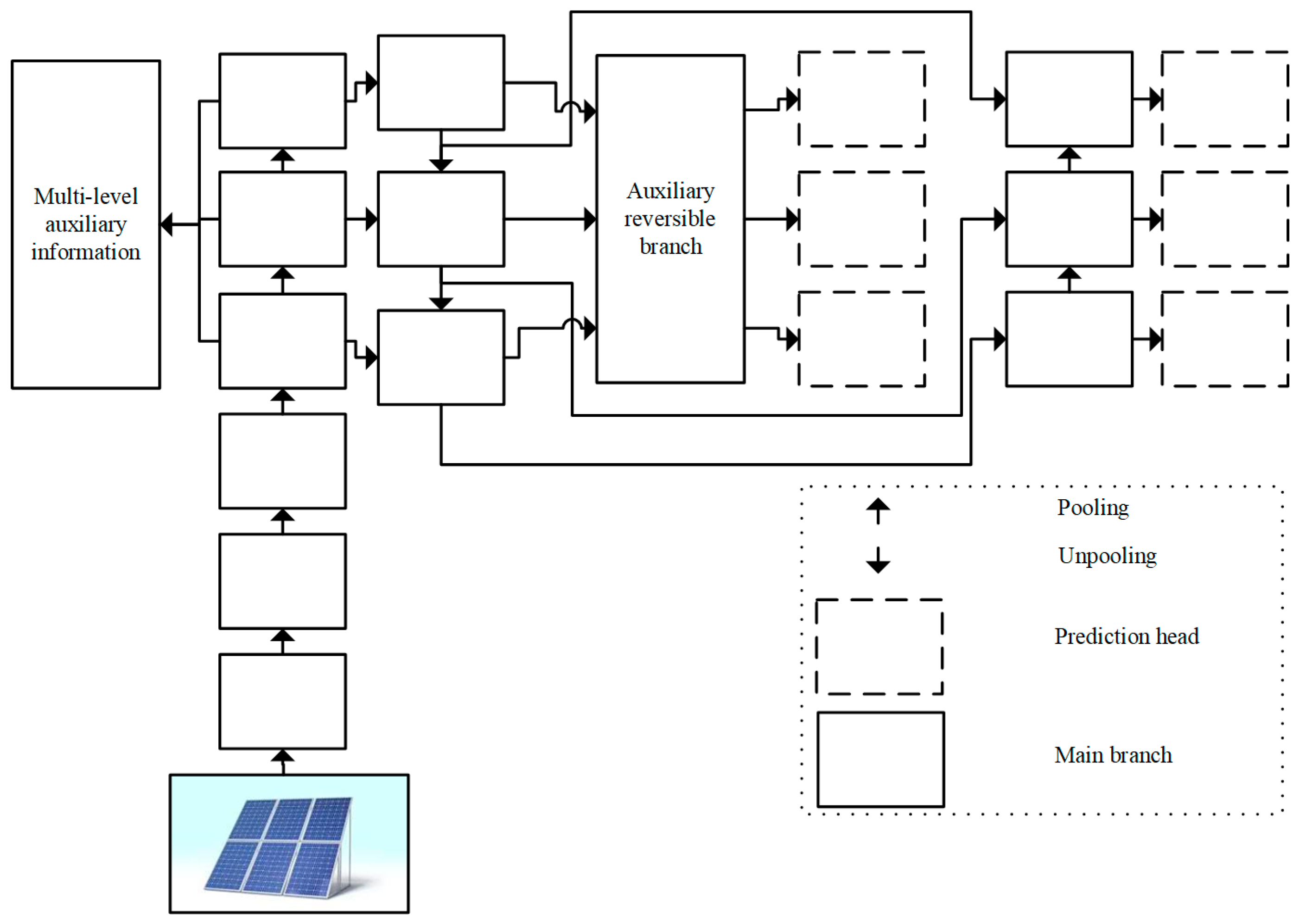
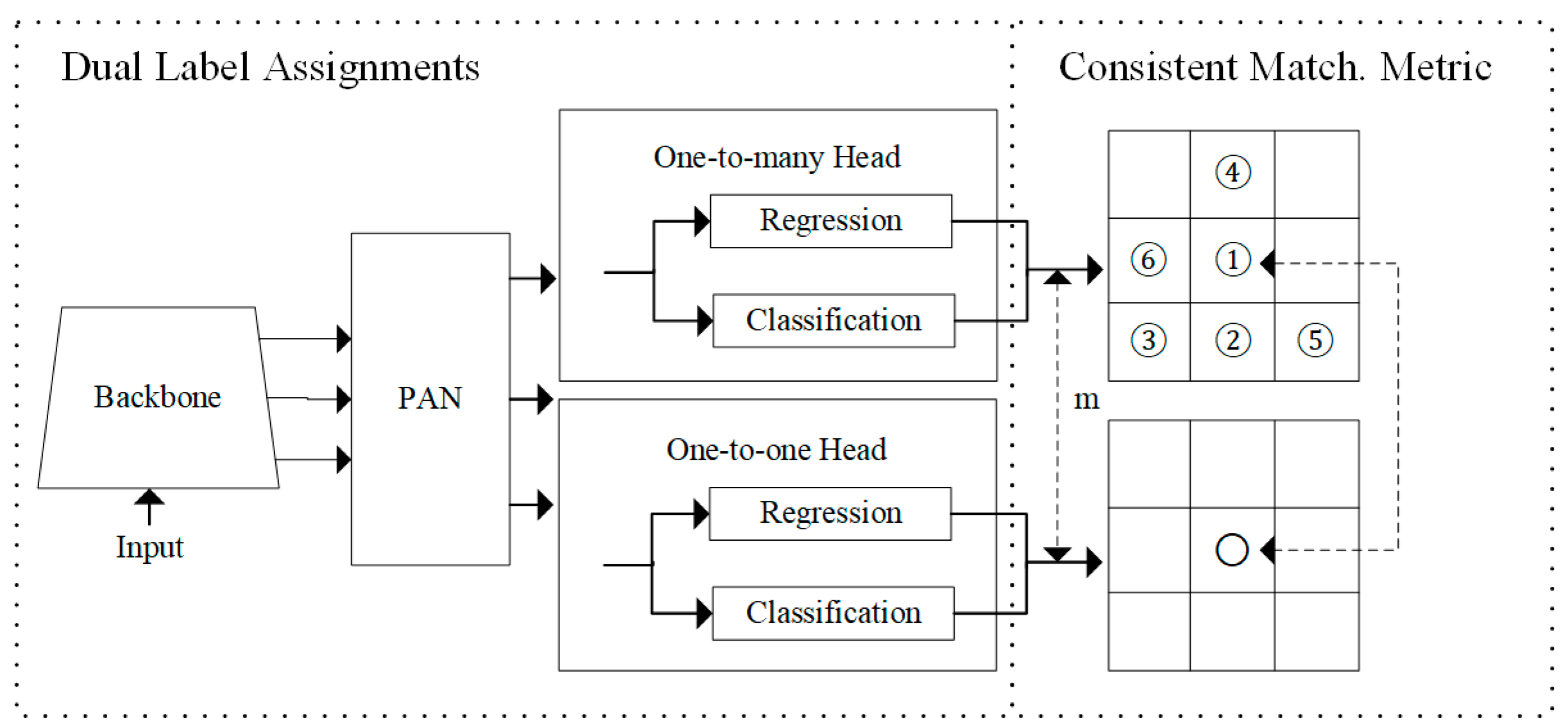
3. YOLO Model
4. Methodology
5. Experimental Evaluation
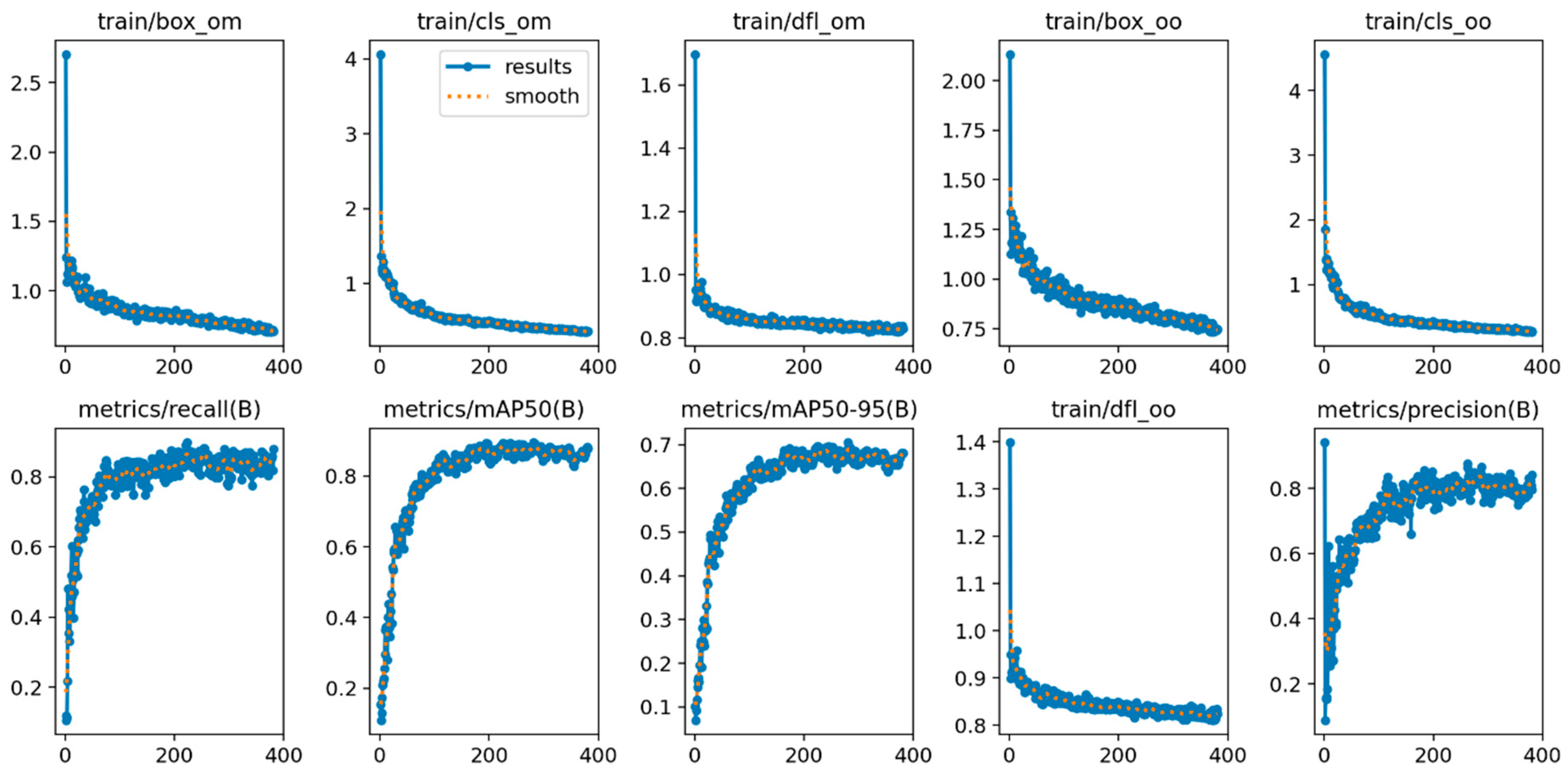
5.1. Training and Validation Results
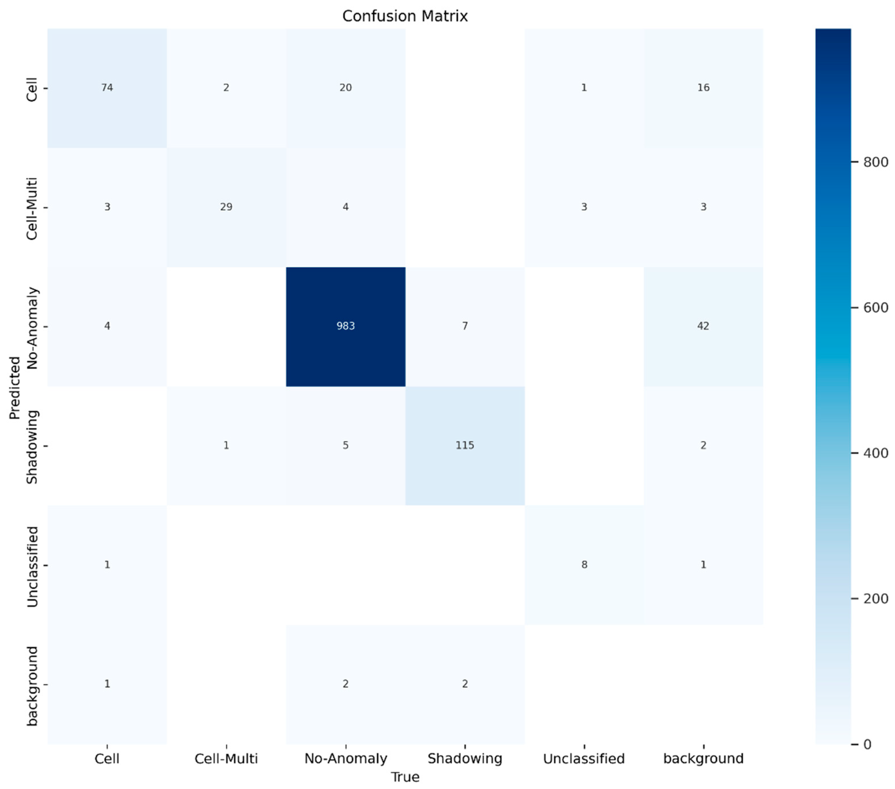
5.2. Test Results
6. Discussion
7. Conclusions and Outlook
Author Contributions
Funding
Data Availability Statement
Conflicts of Interest
References
- IEA. Renewables 2023; IEA: Paris, France, 2023.
- Meribout, M.; Tiwari, V.K.; Herrera, J.P.P.; Baobaid, A.N.M.A. Solar panel inspection techniques and prospects. Measurement 2023, 209, 112466. [Google Scholar] [CrossRef]
- Mohammad, A.; Mahjabeen, F. Revolutionizing solar energy with AI-driven enhancements in photovoltaic technology. BULLET J. Multidisiplin Ilmu 2023, 2, 1174–1187. [Google Scholar]
- Youssef, A.; El-Telbany, M.; Zekry, A. The role of artificial intelligence in photo-voltaic systems design and control: A review. Renew. Sustain. Energy Rev. 2017, 78, 72–79. [Google Scholar] [CrossRef]
- Kermadi, M.; Berkouk, E.M. Artificial intelligence-based maximum power point tracking controllers for Photovoltaic systems: Comparative study. Renew. Sustain. Energy Rev. 2017, 69, 369–386. [Google Scholar] [CrossRef]
- Chine, W.; Mellit, A.; Lughi, V.; Malek, A.; Sulligoi, G.; Pavan, A.M. A novel fault diagnosis technique for photovoltaic systems based on artificial neural networks. Renew. Energy 2016, 90, 501–512. [Google Scholar] [CrossRef]
- Herraiz, Á.H.; Marugán, A.P.; Márquez, F.P.G. Photovoltaic plant condition monitoring using thermal images analysis by convolutional neural network-based structure. Renew. Energy 2020, 153, 334–348. [Google Scholar] [CrossRef]
- Premkumar, M.; Sowmya, R. Certain study on MPPT algorithms to track the global MPP under partial shading on solar PV module/array. Int. J. Comput. Digit. Syst. 2019, 8, 405–416. [Google Scholar] [CrossRef] [PubMed]
- Monicka, S.G.; Manimegalai, D.; Karthikeyan, M. Detection of microcracks in silicon solar cells using Otsu-Canny edge detection algorithm. Renew. Energy Focus 2022, 43, 183–190. [Google Scholar] [CrossRef]
- Bordihn, S.; Fladung, A.; Schlipf, J.; Köntges, M. Machine learning based identification and classification of field-operation caused solar panel failures observed in electroluminescence images. IEEE J. Photovolt. 2022, 12, 827–832. [Google Scholar] [CrossRef]
- Le, M.; Le, D.; Vu, H.H.T. Thermal inspection of photovoltaic modules with deep convolutional neural networks on edge devices in AUV. Measurement 2023, 218, 113135. [Google Scholar] [CrossRef]
- Park, Y.; Kim, M.J.; Gim, U.; Yi, J. Boost-up efficiency of defective solar panel detection with pre-trained attention recycling. IEEE Trans. Ind. Appl. 2023, 59, 3110–3120. [Google Scholar] [CrossRef]
- Vlaminck, M.; Heidbuchel, R.; Philips, W.; Luong, H. Region-based CNN for anomaly detection in PV power plants using aerial imagery. Sensors 2022, 22, 1244. [Google Scholar] [CrossRef]
- Chen, H.; Pang, Y.; Hu, Q.; Liu, K. Solar cell surface defect inspection based on multispectral convolutional neural network. J. Intell. Manuf. 2020, 31, 453–468. [Google Scholar] [CrossRef]
- Duranay, Z.B. Fault detection in solar energy systems: A deep learning approach. Electronics 2023, 12, 4397. [Google Scholar] [CrossRef]
- Di Tommaso, A.; Betti, A.; Fontanelli, G.; Michelozzi, B. A multi-stage model based on YOLOv3 for defect detection in PV panels based on IR and visible imaging by unmanned aerial vehicle. Renew. Energy 2022, 193, 941–962. [Google Scholar] [CrossRef]
- Hassan, S.; Dhimish, M. Enhancing solar photovoltaic modules quality assurance through convolutional neural network-aided automated defect detection. Renew. Energy 2023, 219, 119389. [Google Scholar] [CrossRef]
- Cao, Y.; Pang, D.; Zhao, Q.; Yan, Y.; Jiang, Y.; Tian, C.; Wang, F.; Li, J. Improved yolov8-gd deep learning model for defect detection in electroluminescence images of solar photovoltaic modules. Eng. Appl. Artif. Intell. 2024, 131, 107866. [Google Scholar] [CrossRef]
- Terven, J.; Córdova-Esparza, D.-M.; Romero-González, J.-A. A comprehensive review of yolo architectures in computer vision: From yolov1 to yolov8 and yolo-nas. Mach. Learn. Knowl. Extr. 2023, 5, 1680–1716. [Google Scholar] [CrossRef]
- Solar Panels Computer Vision Project. Available online: https://universe.roboflow.com/roboflow-100/solar-panels-taxvb (accessed on 12 January 2025).
- Afroz. Solar Panel Images Clean and Faulty Images. Available online: https://www.kaggle.com/datasets/pythonafroz/solar-panel-images (accessed on 12 January 2025).
- Wang, C.; Yeh, I.; Liao, H. YOLOv9: Learning what you want to learn using programmable gradient information. arXiv 2024, arXiv:2402.13616. [Google Scholar]
- Jocher, G.; Mattioli, F.; Qaddoumi, B.; Laughing, Q.; Munawar, M.R. YOLOv9: A Leap Forward in Object Detection Technology. Available online: https://docs.ultralytics.com/models/yolov9/ (accessed on 12 January 2025).
- Wang, A.; Chen, H.; Liu, L.; Chen, K.; Lin, Z.; Han, J.; Ding, G. YOLOv10: Real-Time End-to-End Object Detection. arXiv 2024, arXiv:2405.14458. [Google Scholar]
- Khanam, R.; Hussain, M. YOLOv11: An Overview of the Key Architectural Enhancements. arXiv 2024, arXiv:2410.17725. [Google Scholar]
- Bergstra, J.; Bengio, Y. Random search for hyper-parameter optimization. J. Mach. Learn. Res. 2012, 13, 281–305. [Google Scholar]


| The Model | Experiment | Epochs | Batch Size | P | R | mAP50 | mAP (50–95) | F1 Score |
|---|---|---|---|---|---|---|---|---|
| YOLO v5s | 1 | 170 | 2 | 91.4 | 33.3 | 40.7 | 26.4 | 48.8 |
| YOLO v9 | 2 | 162 | 2 | 88.6 | 49.8 | 54.7 | 42.9 | 63.8 |
| YOLO v9 (Trained on Kaggle dataset) | 3 | 150 | 4 | 54.6 | 64.5 | 68 | 61 | 59.1 |
| YOLO v10-X | 4 | 370 | 8 | 81.5 | 85.8 | 89.6 | 70.5 | 83.5 |
| YOLO v10-X (Trained on Kaggle dataset) | 5 | 150 | 32 | 78 | 63.5 | 74.7 | 69.2 | 70 |
| YOLO v11-X | 6 | 150 | 8 | 90.1 | 85.4 | 94.1 | 73.6 | 87.7 |
| YOLO v11-X (Trained on Kaggle dataset) | 7 | 150 | 8 | 54.3 | 68.8 | 67.7 | 63.3 | 60.7 |
| The Model | Experiment | P | R | mAP50 | mAP (50–95) | F1 Score |
|---|---|---|---|---|---|---|
| YOLO v5s | 1 | 55 | 35.9 | 44.6 | 29.3 | 43.4 |
| YOLO v9 | 2 | 94 | 50.3 | 55 | 42.8 | 65.5 |
| YOLO v10-X | 3 | 90.1 | 87.9 | 94.2 | 73.2 | 89 |
| YOLO v11-X | 4 | 90.1 | 86 | 94.1 | 73.3 | 88 |
| The Model | P | R | mAP | F1 Score | Inference Time (ms) |
|---|---|---|---|---|---|
| SVM | 56 | 100 | 56 | 71.8 | 0.6 |
| Faster R-CNN | 62.7 | 85.4 | 62.7 | 72.3 | 3158 |
| YOLO v10-X | 90.1 | 87.9 | 94.2 | 89 | 220.2 |
| YOLO v11-X | 90.1 | 86 | 94.1 | 88 | 252.3 |
| SVM (on Kaggle dataset) | 64 | 100 | 64 | 78 | 1.2 |
| YOLO v10-X (on Kaggle dataset) | 86.6 | 65 | 82.3 | 74.3 | 31.1 |
| YOLO v11-X (on Kaggle dataset) | 58.8 | 72.3 | 69.5 | 65.9 | 58.1 |
| YOLO v11-X (on Aug-RF dataset) | 89.7 | 87.7 | 92.7 | 90 | 149.2 |
Disclaimer/Publisher’s Note: The statements, opinions and data contained in all publications are solely those of the individual author(s) and contributor(s) and not of MDPI and/or the editor(s). MDPI and/or the editor(s) disclaim responsibility for any injury to people or property resulting from any ideas, methods, instructions or products referred to in the content. |
© 2025 by the authors. Licensee MDPI, Basel, Switzerland. This article is an open access article distributed under the terms and conditions of the Creative Commons Attribution (CC BY) license (https://creativecommons.org/licenses/by/4.0/).
Share and Cite
Ghahremani, A.; Adams, S.D.; Norton, M.; Khoo, S.Y.; Kouzani, A.Z. Detecting Defects in Solar Panels Using the YOLO v10 and v11 Algorithms. Electronics 2025, 14, 344. https://doi.org/10.3390/electronics14020344
Ghahremani A, Adams SD, Norton M, Khoo SY, Kouzani AZ. Detecting Defects in Solar Panels Using the YOLO v10 and v11 Algorithms. Electronics. 2025; 14(2):344. https://doi.org/10.3390/electronics14020344
Chicago/Turabian StyleGhahremani, Ali, Scott D. Adams, Michael Norton, Sui Yang Khoo, and Abbas Z. Kouzani. 2025. "Detecting Defects in Solar Panels Using the YOLO v10 and v11 Algorithms" Electronics 14, no. 2: 344. https://doi.org/10.3390/electronics14020344
APA StyleGhahremani, A., Adams, S. D., Norton, M., Khoo, S. Y., & Kouzani, A. Z. (2025). Detecting Defects in Solar Panels Using the YOLO v10 and v11 Algorithms. Electronics, 14(2), 344. https://doi.org/10.3390/electronics14020344