SNR-Based Receiver-Type Decision Using Deep Learning for Multiple-Input Multiple-Output Detection

Abstract

In this paper, we propose a multiple-input multiple-output receiver with deep learning. To obtain the high performance of the maximum likelihood receiver while maintaining the low computational complexity of the linear receiver, we apply a signal-to-noise ratio-based receiver-type decision method. Specifically, the criterion and threshold, which are based on the ratio between the symbol error probabilities of both receivers, to decide the receiver type are presented. For this, we analyze the signal-to-noise ratio gain of the zero-forcing receiver and exploit it as an input feature of the DNN. The simulation results demonstrate that the proposed receiver achieves a symbol error rate performance nearly identical to that of the maximum likelihood receiver with low computational complexity.

1. Introduction

Multiple-input multiple-output (MIMO) systems are widely considered to be a key technologies for wireless communications, as they improve aspects of system performance such as reliability and data rates without requiring additional bandwidth. To take advantage of these facts, MIMO systems have to utilize diversity gain, which can be achieved by various receivers. MIMO receivers can be divided into two categories based on their operation: linear and nonlinear receivers. Linear receivers, such as the zero-forcing (ZF) and minimum mean squared error (MMSE) receivers, have lower computational complexity but suffer from performance degradation. In contrast, nonlinear receivers offer superior error performance but demand significantly higher computational complexity [1,2]. Specifically, the maximum likelihood (ML) receiver requires exponentially increasing computational complexity with the number of transmit antennas, despite providing optimal error performance through brute-force search. To address this problem, detectors such as sphere decoding have been investigated to obtain nearly optimal performance with reasonable computational complexity [3,4].

Recently, artificial intelligence has been studied for various applications in wireless communications such as beamforming, channel estimation, and localization, due to its ability to address non-convex optimization problems [5,6,7,8,9,10,11]. In [5], deep learning is utilized to optimize the antenna position and antenna weight jointly, which is challenging to perform analytically. The authors of [6] proposed a deep learning-based fast beamforming method to solve the sum rate maximization problem. Moreover, in [7], the performances of the deep learning-based channel estimation are analyzed and compared with the conventional channel estimation methods. In [8], deep learning is used to estimate the MIMO channel coefficient for quasi-static block fading and time-varying fading. Deep learning is utilized for 3-D unmanned aerial vehicle localization in [9] by formulating the localization problem as an optimization problem to minimize the error in received signal strength index measurements. The authors of [10] exploit deep learning for indoor localization by converting the localization problem into a classification problem. A deep neural network (DNN)-driven near-field source localization that jointly optimizes the analog beamformer and the localization function is proposed in [11]. Furthermore, artificial intelligence-based approaches have been increasingly employed in MIMO detection to overcome the limitations of conventional receivers [12,13,14,15]. In [12], a deep learning-based scheme is proposed, offering significantly lower computational complexity than the conventional sphere decoding algorithm while achieving near-optimal performance of sphere decoding. The authors of [13] introduced two deep learning networks for MIMO detection named detection network (DetNet) to enable the handling of multiple channels simultaneously with a single training phase and also obtain accuracy comparable to that of sphere decoding with reduced computational complexity. To improve detection performance with imperfect channel state information (CSI), a model-driven deep learning network called the orthogonal approximate message passing (OAMP)-Net2 detector was proposed to jointly perform channel estimation and signal detection in [14]. In [15], a model-driven deep learning-based massive MIMO detector was proposed for multiuser interference cancellation by unfolding an existing iterative algorithm.

Existing studies on MIMO receivers using deep learning have proposed neural network structures for MIMO detection or investigated methods to reduce the computational complexity of conventional nonlinear receivers. Considering that average error performance is mainly affected by large burst errors under poor MIMO channel conditions, it is essential to predict the channel conditions when designing receivers [16]. However, to the best of the authors’ knowledge, most existing studies on MIMO detection with deep learning have not accounted for this issue. To resolve this problem, in this paper, we focus on predicting channel conditions where large burst errors occur and adopting an appropriate receiver to overcome these poor channel conditions. Since complex relationships between the receiver type and various system parameters, such as signal-to-noise ratio (SNR), modulation order, antenna configuration, and MIMO channel characteristics including singular values, cannot be modeled by conventional mathematical approaches, we utilize deep learning, which specializes in modeling complex relationships [17]. We introduce a receiver-type decision method based on the channel conditions by utilizing deep learning. Based on the channel condition, the proposed method adopts the optimal nonlinear receiver for MIMO channels where large burst errors are expected while mainly using the linear receiver. For this, we establish a criterion and threshold for using both types of receivers based on the ratio of symbol error probabilities. Moreover, we present input features for training the DNN by analyzing the SNR gain and describe the operation of the proposed deep learning-based receiver in two phases. Consequently, we can achieve a compromise between the average error performance and reduced computational complexity. In the simulation results, we demonstrate that the proposed receiver chainachieves the same diversity order as the optimal nonlinear receiver, while maintaining low computational complexity, by alternatively using the two types of receivers.

The contributions of this paper are summarized as follows:

• We analyze the average SNR of the linear receiver to predict poor conditioned MIMO channels and present the criterion and threshold of the function for the receiver-type decision.
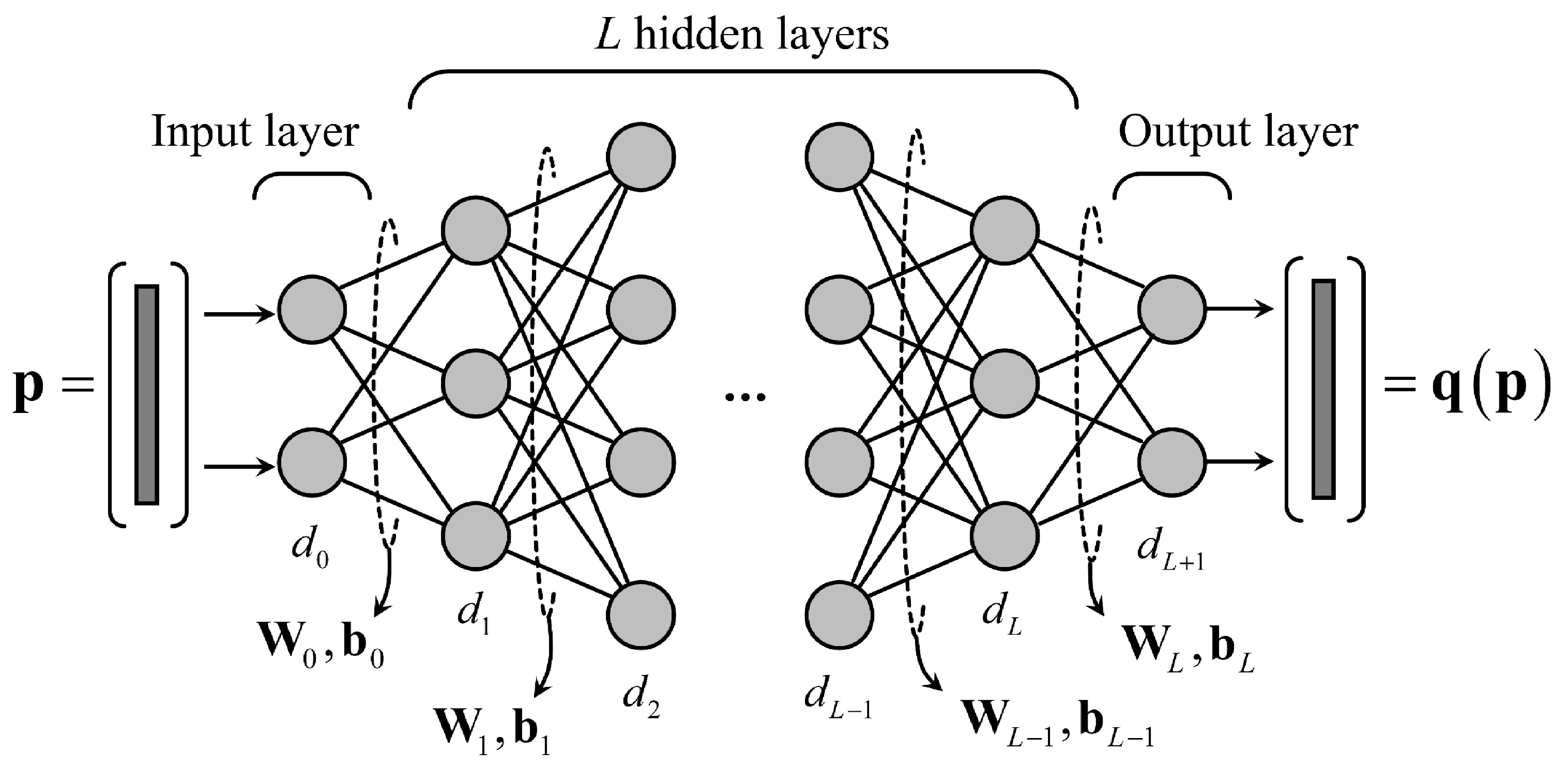
• We introduce the input features of the DNN and propose the DNN structure to model the complex relationship of the presented function.
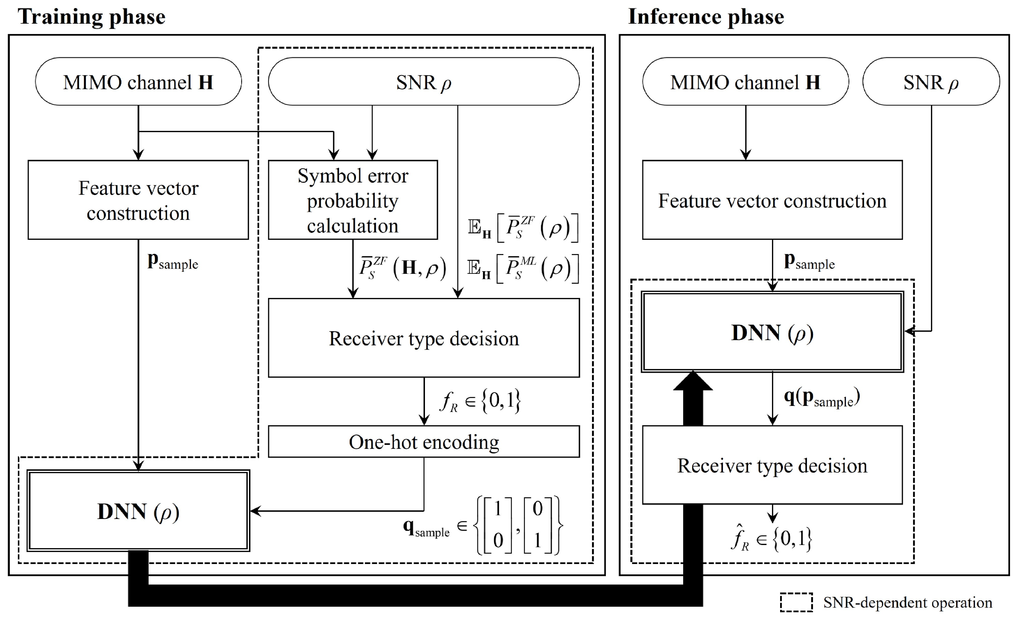
• We present the operation of the deep learning-based proposed receiver in two phases for practical implementation and analyze the computational complexity of the proposed receiver.

2. System Model

We consider a MIMO system where the transmitter and receiver are equipped with $N_T$ and $N_R$ antennas, respectively. Assuming that independent $N_T$ data streams are transmitted, the received signal vector $\mathbf{y}={\left[y_1\cdots y_q\cdots y_{N_R}\right]}^T$ is given by

$$\mathbf{y}=\sqrt{{\displaystyle \frac{E_s}{N_T}}}\mathbf{H}\mathbf{x}+\mathbf{n},$$

(1)

where $E_s$ denotes the average transmit energy over a symbol duration, $\mathbf{H}$ is an $N_R\times N_T$ MIMO channel matrix, $\mathbf{x}={\left[x_1\cdots x_p\cdots x_{N_T}\right]}^T$ is an $N_T\times 1$ transmitted signal vector with $\mathbb{E}\left[\mathbf{x}{\mathbf{x}}^H\right]={\mathbf{I}}_{N_T}$, $\mathbf{n}={\left[n_1\cdots n_q\cdots n_{N_R}\right]}^T$ represents an $N_R\times 1$ additive white Gaussian noise vector that satisfies $\mathbb{E}\left[\mathbf{n}{\mathbf{n}}^H\right]=N_0{\mathbf{I}}_{N_R}$, and $N_0$ is a noise spectral density. A $\left(q,p\right)$ element of the channel matrix $\mathbf{H}$, ${\left\{\mathbf{H}\right\}}_{q,p}=h_{qp}$, is the channel coefficient between the pth transmit antenna and qth receive antenna, where ${\left\{·\right\}}_{q,p}$ represents the element at qth row and pth column. We assume that $h_{qp}$ is an independently and identically distributed complex Gaussian random variable with zero mean and unit variance [1].

A linear receiver can be considered to reduce the computational complexity at the receiver in detecting the transmitted signal vector $\mathbf{x}$, and in this paper, we adopt a ZF receiver that is one of the linear receivers. Using the ZF receiver, the post-processing signal vector ${\mathbf{z}}^{ZF}$ is given by

$$\begin{array}{cc}\hfill {\mathbf{z}}^{ZF}& =\sqrt{{\displaystyle \frac{N_T}{E_s}}}{\mathbf{H}}^{†}\mathbf{y}\hfill \\ \hfill & =\mathbf{x}+\sqrt{{\displaystyle \frac{N_T}{E_s}}}{\mathbf{H}}^{†}\mathbf{n},\hfill \end{array}$$

(2)

where ${\mathbf{H}}^{†}$ represents the Moore–Penrose inverse. Note that $N_R\ge N_T$ is required for the ZF receiver to be feasible and, accordingly, ${\mathbf{H}}^{†}={\left({\mathbf{H}}^H\mathbf{H}\right)}^{-1}{\mathbf{H}}^H$ [18]. In (2), the demodulated signal corresponding to the pth transmitted signal, ${\widehat{x}}_p^{ZF}$, is obtained by the following metric:

$${\widehat{x}}_p^{ZF}=\underset{s\in \mathcal{S}}{argmin}\left|z_p^{ZF}-s\right|,$$

(3)

where $\mathcal{S}$ represents a set of signal constellation points whose cardinality is $\left|\mathcal{S}\right|=M$ [1]. Besides, for the given MIMO channel $\mathbf{H}$, the symbol error probability can be expressed as

$${\overline{P}}_S^{ZF}\left(\rho ,\mathbf{H}\right)={\displaystyle \frac{1}{N_T}}\sum _{p=1}^{N_T}\sum _{s\in \mathcal{S}}Pr\left[x_p=s\right]Pr\left[{\widehat{x}}_p^{ZF}\ne x_p|x_p=s,\mathbf{H}\right],$$

(4)

where $\rho ={\displaystyle \frac{E_s}{N_0}}$ is the average transmit SNR. Since the transmitted signal from each transmit antenna can be detected independently, the ZF receiver has a computational complexity depending on $M{N}_T$, which grows linearly with $N_T$ [1]. However, the ZF receiver can obtain only $N_R-N_T+1$ of diversity order due to the utilization of degrees of freedom in the matrix inversion process [19].

On the other hand, we also consider applying an ML receiver, which is a well-known optimal receiver for MIMO detection. Exploiting the ML receiver, the demodulated signal vector ${\widehat{\mathbf{x}}}^{ML}={\left[{\widehat{x}}_1^{ML}\cdots {\widehat{x}}_p^{ML}\cdots {\widehat{x}}_{N_T}^{ML}\right]}^T$ is obtained by the following metric:

$${\widehat{\mathbf{x}}}_p^{ML}=\underset{s\in {\mathcal{S}}_{ML}}{argmin}{∥\mathbf{y}-\sqrt{{\displaystyle \frac{E_s}{N_T}}}\mathbf{H}\mathbf{s}∥}_F^2,$$

(5)

where ${\mathcal{S}}_{ML}$ is a set of candidate vectors for the ML receiver whose cardinality is $\left|{\mathcal{S}}_{ML}\right|=M^{N_T}$. Similar to the ZF receiver, for the given MIMO channel $\mathbf{H}$, we can express the symbol error probability of the ML receiver as follows [20]:

$${\overline{P}}_S^{ZF}\left(\rho ,\mathbf{H}\right)={\displaystyle \frac{1}{N_T}}\sum _{p=1}^{N_T}\sum _{s\in \mathcal{S}}Pr\left[x_p=s\right]Pr\left[{\widehat{x}}_p^{ML}\ne x_p|x_p=s,\mathbf{H}\right].$$

(6)

Considering (5), $M^{N_T}$ searches through all candidates in ${\mathcal{S}}_{ML}$ are necessary, and this results in exponentially increasing computational complexity with $N_T$. Instead, the ML receiver can achieve an $N_R$ diversity order, potentially resulting in better error performance compared to the ZF receiver.

3. Proposed Deep Learning-Based MIMO Receiver

Thanks to the optimality of the ML decision rule, the ML receiver can achieve optimal error performance [21]. However, as explained in Section 2, it demands significantly high computational complexity, which can be critical in scenarios where the receiver must operate with limited battery power [22]. The linear receiver can be straightforwardly exploited in MIMO detection with much lower computational complexity, even though it suffers from performance loss, particularly in poorly conditioned channels [23,24]. To obtain the advantages of both receivers, we propose a MIMO receiver that adopts the two types of receivers alternatively and present the operation method of the proposed receiver. Especially, deep learning is exploited for the proposed receiver to identify the receiver type according to the characteristics of the MIMO channels.

3.1. Threshold for Receiver-Type Decision

The ZF receiver is one of the most widely investigated linear receivers in which the multi-stream interference can be eliminated. However, as shown in (2), the post-processing signal suffers from noise enhancement depending on the MIMO channel matrix $\mathbf{H}$. In (2), ${\left\{{\mathbf{z}}^{ZF}\right\}}_p=z_p^{ZF}$, which corresponds to the transmitted signal of the pth transmit antenna, is given by

$$z_p^{ZF}=x_p+\sqrt{{\displaystyle \frac{N_T}{E_s}}}{\left\{{\left({\mathbf{H}}^H\mathbf{H}\right)}^{-1}{\mathbf{H}}^H\mathbf{n}\right\}}_p.$$

(7)

Denoting $\mathbf{G}=\left[{\mathbf{g}}_1\cdots {\mathbf{g}}_p\cdots {\mathbf{g}}_{N_T}\right]=\mathbf{H}{\left({\mathbf{H}}^H\mathbf{H}\right)}^{-1}$, (7) can be rewritten by

$$z_p^{ZF}=x_p+\sqrt{{\displaystyle \frac{N_T}{E_s}}}{\mathbf{g}}_p^H\mathbf{n}.$$

(8)

Then, the average SNR for the pth demodulated signal can be calculated as follows [25]:

$$\begin{array}{cc}\hfill {\rho }_p& ={\displaystyle \frac{\mathbb{E}\left[{\left|x_p\right|}^2\right]}{\mathbb{E}\left[\frac{N_T}{E_s}{\left|{\mathbf{g}}_p^H\mathbf{n}\right|}^2\right]}}\hfill \\ \hfill & ={\displaystyle \frac{E_s}{N_T{N}_0}}{\displaystyle \frac{1}{{∥{\mathbf{g}}_p∥}_F^2}}\hfill \\ \hfill & ={\displaystyle \frac{\rho }{N_T}}{\displaystyle \frac{1}{{\left\{{\mathbf{G}}^H\mathbf{G}\right\}}_{p,p}}}\hfill \\ \hfill & ={\displaystyle \frac{\rho }{N_T}}{\displaystyle \frac{1}{{\left\{{\left({\mathbf{H}}^H\mathbf{H}\right)}^{-1}\right\}}_{p,p}}}.\hfill \end{array}$$

(9)

Applying the singular value decomposition (SVD) of the MIMO channel $\mathbf{H}=\mathbf{U}\Sigma {\mathbf{V}}^H$, ${\rho }_p$ in (9) can be rewritten as

$$\begin{array}{cc}\hfill {\rho }_p& ={\displaystyle \frac{\rho }{N_T}}{\displaystyle \frac{1}{{\left\{{\sum }_{i=1}^{N_T}{\sigma }_i^{-2}{\mathbf{v}}_i{\mathbf{v}}_i^H\right\}}_{p,p}}}\hfill \\ \hfill & ={\displaystyle \frac{\rho }{N_T}}{\displaystyle \frac{1}{{\sum }_{i=1}^{N_T}{\sigma }_i^{-2}{\left|{\left\{{\mathbf{v}}_i\right\}}_p\right|}^2}},\hfill \end{array}$$

(10)

where $\mathbf{U}=\left[{\mathbf{u}}_1\cdots {\mathbf{u}}_q\cdots {\mathbf{u}}_{N_R}\right]$ and $\mathbf{V}=\left[{\mathbf{v}}_1\cdots {\mathbf{v}}_p\cdots {\mathbf{v}}_{N_T}\right]$ are matrices including left singular vectors and right singular vectors, respectively, and ${\sigma }_p={\left\{\Sigma \right\}}_{p,p}$ denotes the pth largest singular value of $\mathbf{H}$. As shown in (10), the average SNR for each demodulated signal is determined by the distribution of singular values and right singular vectors. For ease of analysis, we assume that ${\left|{\left\{{\mathbf{v}}_1\right\}}_p\right|}^2=\cdots ={\left|{\left\{{\mathbf{v}}_{N_T}\right\}}_p\right|}^2=v^2$. Then, the derived result in (10) is a harmonic mean of ${\displaystyle \frac{\rho }{N_T^2{v}^2}}{\sigma }_1^2,\cdots ,{\displaystyle \frac{\rho }{N_T^2{v}^2}}{\sigma }_{N_T}^2$. Applying the inequality between the arithmetic mean and harmonic mean, we can obtain the upper-bound of (10) as

$${\rho }_p\le {\displaystyle \frac{\rho }{N_T^3{v}^2}}\sum _{i=1}^{N_T}{\sigma }_i^2,$$

(11)

where the equality holds when ${\sigma }_1=\cdots ={\sigma }_{N_T}$. As mentioned at the beginning of this section, it implies that there are poorly conditioned MIMO channels, which indicates that ${\sigma }_{N_T}\ll {\sigma }_1$ experience SNR loss due to critical noise enhancement.

In (10), it can be stated that the error performance of the ZF receiver depends on the MIMO channel $\mathbf{H}$. Therefore, we propose a receiver that decides the receiver type based on whether the ZF receiver can guarantee a certain level of symbol error rate (SER). To this end, we define a criterion for the receiver-type decision that compares the average SER of the ZF receiver with a threshold $\eta$. Consider a function $f_R\in \left\{0,1\right\}$ for the receiver type, where $f_R=1$ and $f_R=0$ indicate the use of the ZF receiver and ML receiver, respectively. Then, $f_R$ can be expressed as

$$f_R=\left\{\begin{array}{cc}\hfill 0;& {\overline{P}}_S^{ZF}\left(\rho ,\mathbf{H}\right)>\eta ,\hfill \\ \hfill 1;& {\overline{P}}_S^{ZF}\left(\rho ,\mathbf{H}\right)\le \eta .\hfill \end{array}\right.$$

(12)

To ensure the proposed receiver guarantees a certain level of error performance compared to the SER of the ML receiver, we set the threshold $\eta$ as follows:

$$\eta =\gamma {\mathbb{E}}_{\mathbf{H}}\left[{\overline{P}}_S^{ML}\left(\rho ,\mathbf{H}\right)\right],$$

(13)

where $\gamma$ denotes the scaling factor for the threshold $\eta$. In (13), ${\mathbb{E}}_{\mathbf{H}}\left[·\right]$ represents an expectation over $\mathbf{H}$, so ${\mathbb{E}}_{\mathbf{H}}\left[{\overline{P}}_S^{ML}\left(\rho ,\mathbf{H}\right)\right]$ can be calculated by the average of ${\overline{P}}_S^{ML}\left(\rho ,\mathbf{H}\right)$ over a number of channel realizations. Substituting (13) into (12), $f_R$ is rewritten as

$$f_R=\left\{\begin{array}{cc}\hfill 0;& {\displaystyle \frac{{\overline{P}}_S^{ZF}\left(\rho ,\mathbf{H}\right)}{{\mathbb{E}}_{\mathbf{H}}\left[{\overline{P}}_S^{ML}\left(\rho ,\mathbf{H}\right)\right]}}>\gamma ,\hfill \\ \hfill 1;& {\displaystyle \frac{{\overline{P}}_S^{ZF}\left(\rho ,\mathbf{H}\right)}{{\mathbb{E}}_{\mathbf{H}}\left[{\overline{P}}_S^{ML}\left(\rho ,\mathbf{H}\right)\right]}}\le \gamma .\hfill \end{array}\right.$$

(14)

As explained in Section 2, the ZF receiver and ML receiver have $N_R-N_T+1$ and $N_R$ of diversity order, respectively, and this implies that the gap in SER performance between the two receivers widens as the SNR increases. To reflect the SER gap according to SNR, we set the scaling factor $\gamma$ as follows:

$$\gamma =\alpha {\left({\displaystyle \frac{{\mathbb{E}}_{\mathbf{H}}\left[{\overline{P}}_S^{ML}\right]}{{\mathbb{E}}_{\mathbf{H}}\left[{\overline{P}}_S^{ZF}\right]}}\right)}^{\beta },$$

(15)

where $\alpha$ and $\beta$ represent a coefficient and exponent depending on the system parameters such as antenna configurations and modulation order, respectively.

3.2. Deep Learning-Based Operation

We aim to decide the receiver type for the given MIMO channel $\mathbf{H}$, but it is challenging to analyze $f_R$ in (14) mathematically. Therefore, we utilize deep learning to represent the relationship between $\mathbf{H}$ and $f_R$. To increase learning accuracy, it is possible to use a feature vector $\mathbf{p}$ that includes not only MIMO channel coefficients but also various properties of the MIMO channel matrix $\mathbf{H}$. In other words, our goal is to model the relationship between the feature vector $\mathbf{p}$ and $f_R\left(\mathbf{p}\right)$ using DNN.

We consider a DNN structure consisting of L hidden layers, and each layer has $d_1,d_2,\cdots ,d_L$ nodes, as described in Figure 1. The output of lth layer, $l=1,2,\cdots ,L+1$ is given by

$${\mathbf{r}}_l={\varphi }_l\left({\mathbf{W}}_{l-1}{\mathbf{r}}_{l-1}+{\mathbf{b}}_{l-1}\right),$$

(16)

where ${\varphi }_l\left(·\right)$, ${\mathbf{W}}_l\in {\mathbb{R}}^{d_l\times d_{l+1}}$, ${\mathbf{b}}_l\in {\mathbb{R}}^{d_{l+1}}$ are the activation function, weight matrix, and bias vector of lth layer, respectively. Without a loss of generality, ${\mathbf{r}}_0$ and ${\mathbf{r}}_{L+1}$ indicate the input and output vector of the DNN, respectively, and the number of nodes of each vector is $d_0$ and $d_{L+1}$, respectively. As the activation functions, we adopt the rectified linear unit (ReLU) for the input layer and hidden layers. Namely, the ith element of the output vector of $l^{\prime }$th layer, ${\left\{{\mathbf{r}}_{l^{\prime }}\right\}}_i$, $l^{\prime }=1,2,\cdots ,L$, $i=1,2,\cdots ,d_{l^{\prime }}$, is given by

$${\left\{{\mathbf{r}}_{l^{\prime }}\right\}}_i=max\left\{0,{\left\{{\mathbf{W}}_{l^{\prime }-1}{\mathbf{r}}_{l^{\prime }-1}+{\mathbf{b}}_{l^{\prime }-1}\right\}}_i\right\}.$$

(17)

For the activation function of the output layer, we use the softmax function since the DNN is designed for the classification problem for the receiver-type decision. The ith element of the output vector, ${\left\{{\mathbf{r}}_{L+1}\right\}}_i$, $i=1,2,\cdots ,d_{L+1}$, is expressed as

$${\left\{{\mathbf{r}}_{L+1}\right\}}_i={\displaystyle \frac{exp\left({\left\{{\mathbf{W}}_L{\mathbf{r}}_L+{\mathbf{b}}_L\right\}}_i\right)}{{\sum }_{j=1}^{d_{L+1}}exp\left({\left\{{\mathbf{W}}_L{\mathbf{r}}_L+{\mathbf{b}}_L\right\}}_j\right)}}.$$

(18)

Note that $d_{L+1}=2$ since the number of possible $f_R$ is 2.

For the data samples to train the DNN, consider the input and output vector by ${\mathbf{p}}_{\mathrm{sample}}={\mathbf{r}}_0\in {\mathbb{R}}^{d_0}$ and ${\mathbf{q}}_{\mathrm{sample}}\in {\mathbb{R}}^{d_{L+1}}$ for the given MIMO channel $\mathbf{H}$. As mentioned above, ${\mathbf{p}}_{\mathrm{sample}}$ should include properties of $\mathbf{H}$ as features that help improve learning accuracy. Based on the average SNR of the demodulated signal in (9), we consider the SNR gain for $N_T$ transmitted signals as a feature. Let us define $G_p$ as the SNR gain for pth transmitted signal. According to (9), $G_p$ can be expressed as

$$G_p={\displaystyle \frac{1}{{\left\{{\left({\mathbf{H}}^H\mathbf{H}\right)}^{-1}\right\}}_{p,p}}}.$$

(19)

Then, we construct the input feature vector ${\mathbf{p}}_{\mathrm{sample}}$ as follows:

$${\mathbf{p}}_{\mathrm{sample}}={\left[\mathrm{Re}\left\{\mathrm{vec}{\left(\mathbf{H}\right)}^T\right\}\mathrm{Im}\left\{\mathrm{vec}{\left(\mathbf{H}\right)}^T\right\}{G}_1{G}_2\cdots G_{N_T}\right]}^T.$$

(20)

Note that we make every element of the feature vector ${\mathbf{p}}_{\mathrm{sample}}$ a real number by vectorizing the real and imaginary parts of $\mathbf{H}$ and stacking them since the weight matrices and bias vectors of the DNN are defined in the real domain. Moreover, we utilize the one-hot-encoding for construct ${\mathbf{q}}_{\mathrm{sample}}$, which is determined by $f_R\left({\mathbf{p}}_{\mathrm{sample}}\right)$ as follows [26]:

$${\mathbf{q}}_{\mathrm{sample}}=\left\{\begin{array}{cc}\hfill \left[1,0\right];& f_R\left({\mathbf{p}}_{\mathrm{sample}}\right)=0,\hfill \\ \hfill \left[0,1\right];& f_R\left({\mathbf{p}}_{\mathrm{sample}}\right)=1.\hfill \end{array}\right.$$

(21)

where $f_R\left({\mathbf{p}}_{\mathrm{sample}}\right)$ can be obtained by (14). With ${\mathbf{p}}_{\mathrm{sample}}$, we have $\mathbf{q}\left({\mathbf{p}}_{\mathrm{sample}}\right)={\mathbf{r}}_{L+1}$. A well-trained DNN indicates that the difference between ${\mathbf{r}}_{L+1}$ and ${\mathbf{q}}_{\mathrm{sample}}$ is sufficiently small. Therefore, we update the weight matrices and bias vectors to decrease the loss function $\mathcal{L}$. As the loss function $\mathcal{L}$ for the proposed receiver, we use the cross-entropy between ${\mathbf{q}}_{\mathrm{sample}}$ and $\mathbf{q}\left({\mathbf{p}}_{\mathrm{sample}}\right)$ as follows [17]:

$$\mathcal{L}=-{\displaystyle \frac{1}{2}}\sum _{i=1}^2{\left\{{\mathbf{q}}_{\mathrm{sample}}\right\}}_i{log}_2\left({\left\{{\mathbf{q}}_{\mathrm{sample}}\right\}}_i\right).$$

(22)

Since the proposed receiver operates based on the DNN, it is important to sufficiently train the DNN using a large number of labeled data to ensure accurate prediction. Based on the input–output relationship above, as depicted in Figure 2, we proposed that the receiver operates in two phases: a training phase where the DNN is trained, and an inference phase where the receiver type is determined with well-trained DNN. In the training phase, for the given channel $\mathbf{H}$, ${\mathbf{p}}_{\mathrm{sample}}$ is generated at the receiver by (20). Moreover, to obtain ${\mathbf{q}}_{\mathrm{sample}}$, the proposed receiver calculates ${\overline{P}}_S^{ZF}\left(\mathbf{H}\right)$ to determine $f_R$ using (14), assuming that the receiver has empirically ${\mathbb{E}}_{\mathbf{H}}\left[{\overline{P}}_S^{ML}\left(\mathbf{H}\right)\right]$ in advance. The receiver constructs the ${\mathbf{q}}_{\mathrm{sample}}$ based on (21) and then updates the DNN parameters. Note that the proposed receiver repeats this operation for numerous channel realizations in the training phase to train the DNN sufficiently. In the inference phase, with well-trained DNN, the proposed receiver generates ${\mathbf{p}}_{\mathrm{sample}}$ for the given MIMO channel $\mathbf{H}$ and achieves $\mathbf{q}\left({\mathbf{p}}_{\mathrm{sample}}\right)$. Since the $\mathbf{q}\left({\mathbf{p}}_{\mathrm{sample}}\right)$ is obtained by applying the softmax function and each element of $\mathbf{q}\left({\mathbf{p}}_{\mathrm{sample}}\right)$ indicates its probability, the proposed receiver determines the receiver type in the inference phase ${\widehat{f}}_R$ as follows:

$${\widehat{f}}_R=\left\{\begin{array}{cc}\hfill 0;& {\left\{\mathbf{q}\left({\mathbf{p}}_{\mathrm{sample}}\right)\right\}}_1>{\left\{\mathbf{q}\left({\mathbf{p}}_{\mathrm{sample}}\right)\right\}}_0,\hfill \\ \hfill 1;& {\left\{\mathbf{q}\left({\mathbf{p}}_{\mathrm{sample}}\right)\right\}}_1\le {\left\{\mathbf{q}\left({\mathbf{p}}_{\mathrm{sample}}\right)\right\}}_0.\hfill \end{array}\right.$$

(23)

Consequently, the ML receiver is adopted when ${\widehat{f}}_R=0$ and the ZF receiver is used when ${\widehat{f}}_R=1$.

3.3. Complexity Analysis

Let $N_{ZF}$ be the number of times the ZF receiver is used out of N channel realizations during the inference phase, and $N_{ML}=N-N_{ZF}$ be the number of times the ML receiver is adopted. Then, the average number of candidate searches in the demodulation process that determines the computational complexity of the proposed receiver is given by

$$C_{\mathrm{proposed}}={\displaystyle \frac{N_{ZF}}{N}}{C}_{ZF}+{\displaystyle \frac{N_{ML}}{N}}{C}_{ML}.$$

(24)

We use the number of real multiplications required for symbol replica generation and the calculation of squared Euclidean distance with the M modulation order as the measure of the computational complexity of both receivers, $C_{ML}$ and $C_{ZF}$. According to [27,28], the ML receiver requires $4N_T{N}_{R}M$ and $2N_R{M}^{N_T}$ real multiplications for symbol replica generation and the calculation of squared Euclidean distance, respectively. Therefore, we use $C_{ML}$ in (24) by $4N_T{N}_{R}M+2N_R{M}^{N_T}$. On the other hand, for the ZF case, M and $2M$ real multiplications are required for symbol replica generation and the calculation of squared Euclidean distance, respectively. Since those real multiplications are necessary for each data stream, we use $C_{ZF}$ in (24) by $3N_{T}M$. Consequently, the computational complexity of the proposed receiver can be expressed by

$$C_{\mathrm{proposed}}={\displaystyle \frac{3N_{ZF}}{N}}{N}_{T}M+{\displaystyle \frac{N_{ML}}{N}}\left(4N_T{N}_{R}M+2N_R{M}^{N_T}\right).$$

(25)

Considering that the ML receiver is adopted if the ZF receiver cannot guarantee a certain level of SER performance when the MIMO channel is given, increasing the threshold $\eta$ leads to higher $N_{ZF}$. Namely, using a value of $\eta$ that is too large or too small would cause the proposed receiver to operate as the ZF receiver or the ML receiver, respectively. Therefore, it is important to use the appropriate threshold to compromise between error performance and computational complexity.

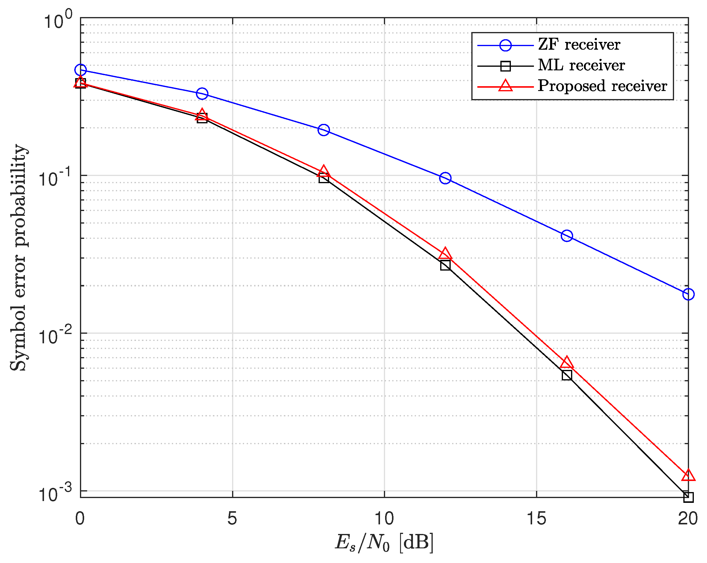
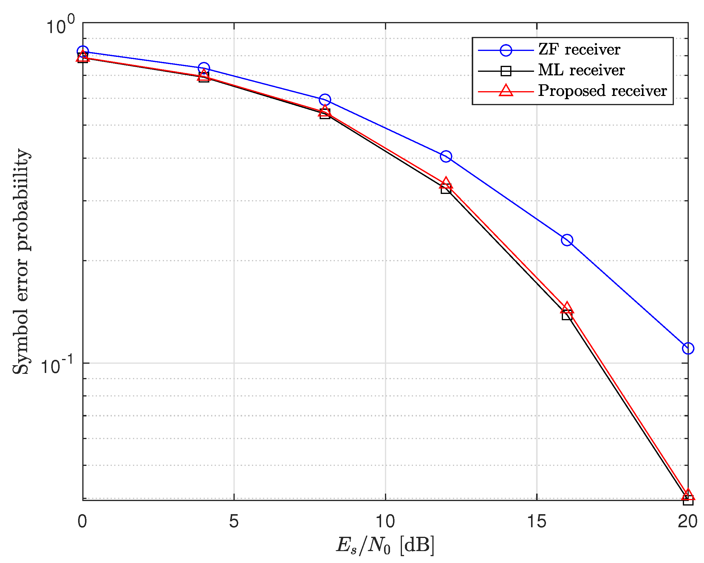
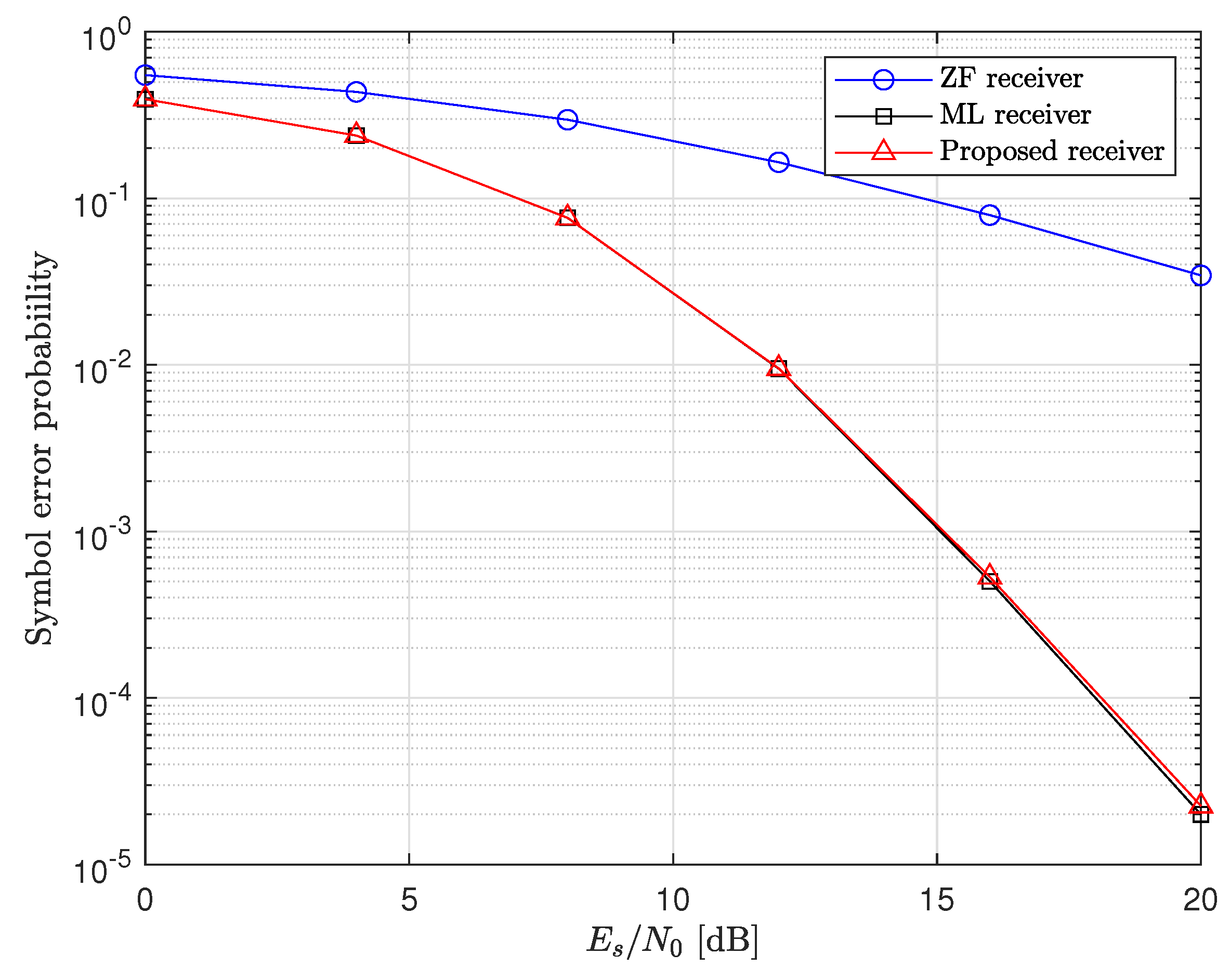
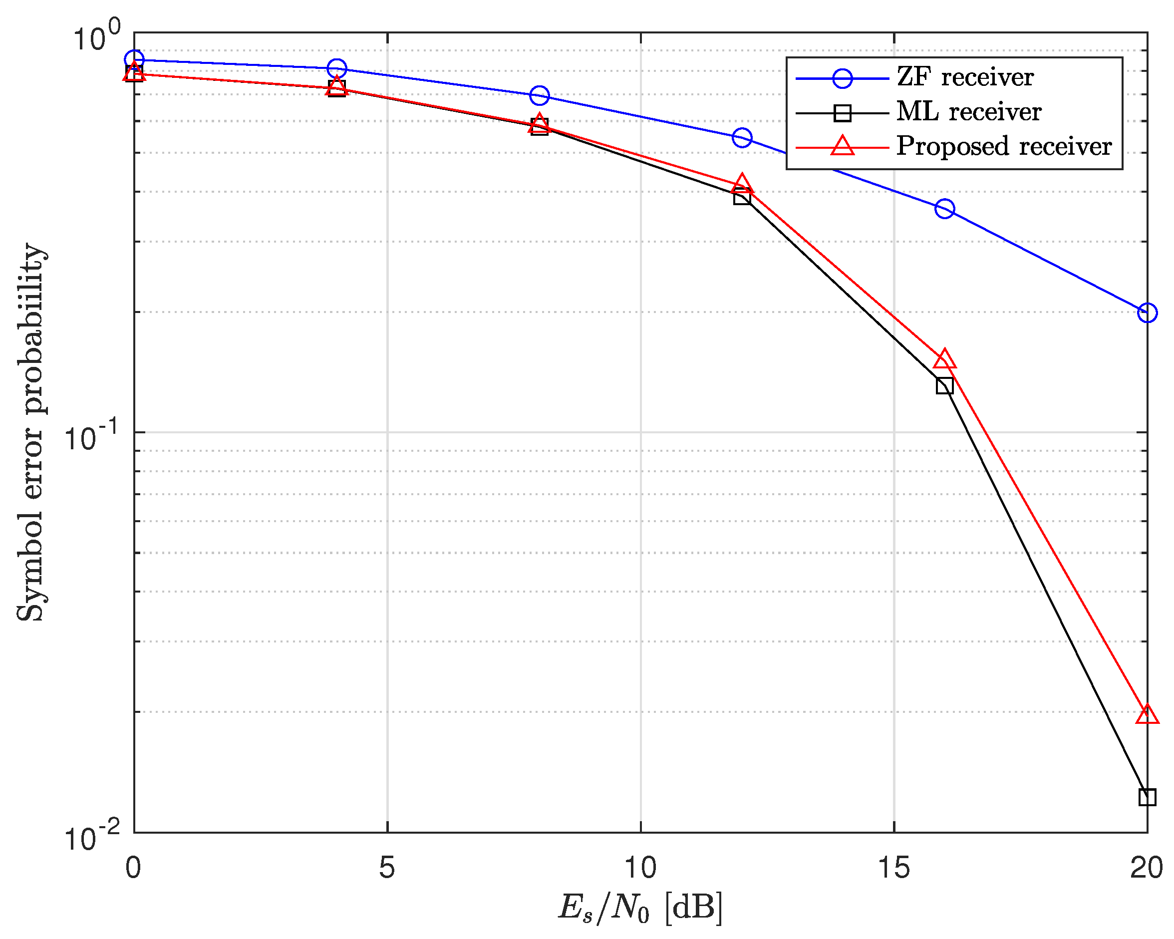
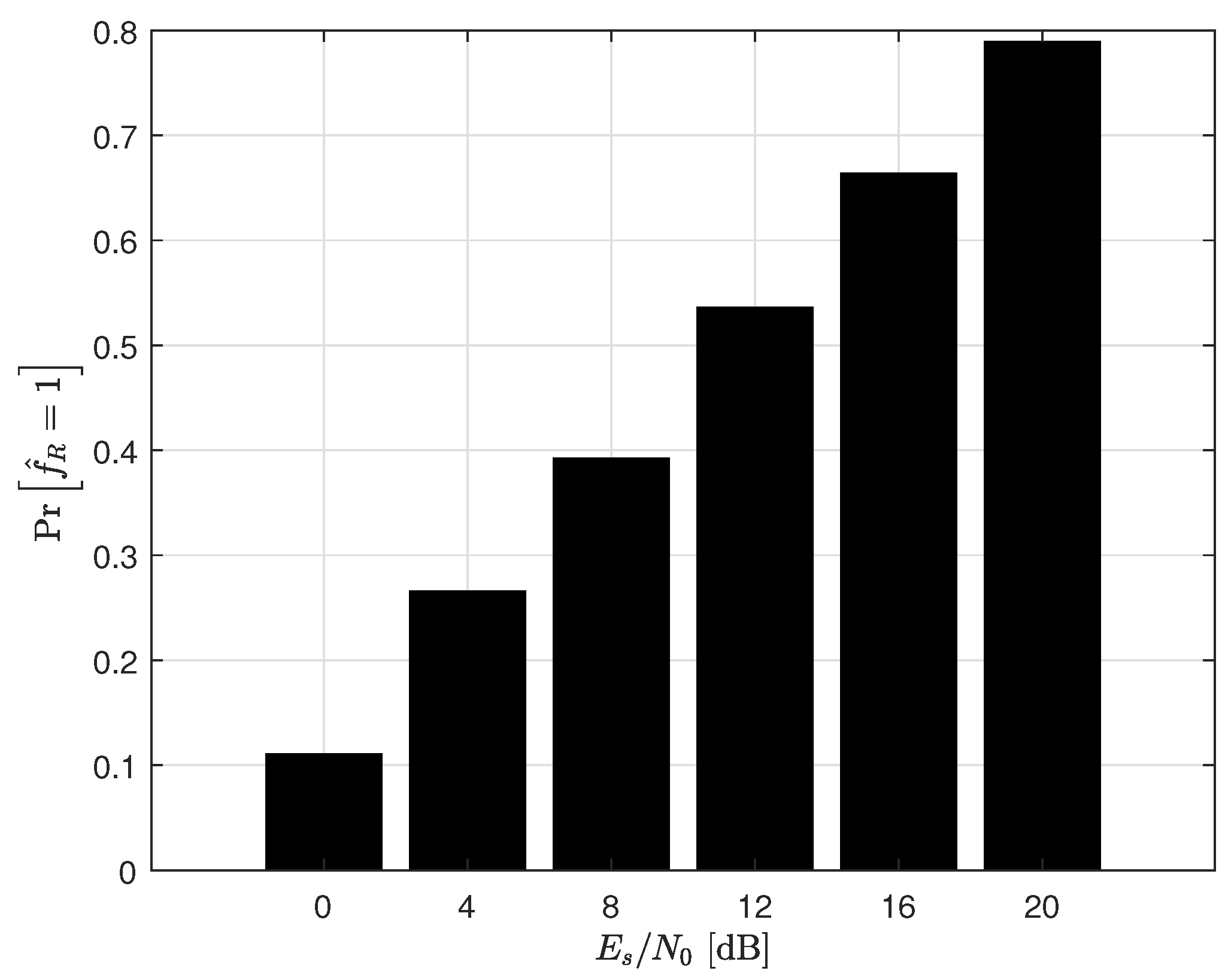
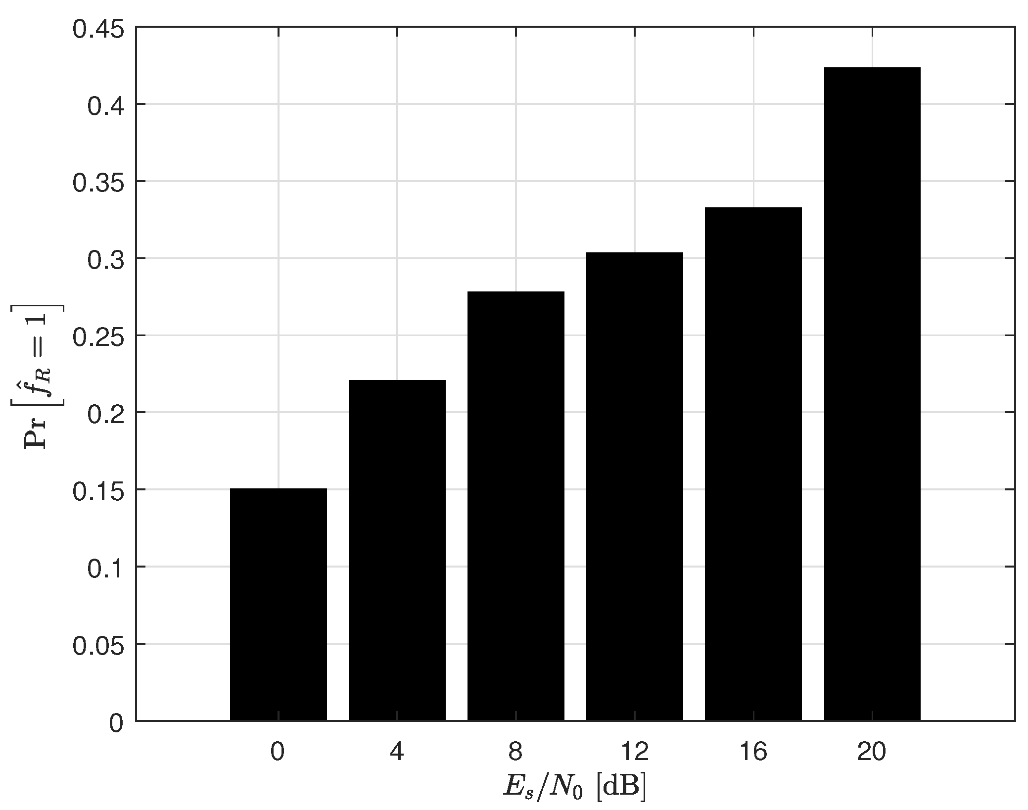
4. Simulation Results

In this section, we provide simulation results for a $2\times 2$ and $4\times 4$ MIMO system with 4−QAM and 16−QAM to evaluate the performance of the proposed receiver. The system parameters and DNN hyperparameters are summarized in

Table 1. System parameters for simulations.

Parameters	Values
Number of transmit antennas, $N_T$	2, 4
Number of receiver antennas, $N_R$	2, 4
Modulation scheme	QAM
Modulation order, M	4, 16
Energy per symbol to noise spectral density ratio, ${\displaystyle \frac{E_s}{N_0}}=\rho$	0, 4, 8, 12, 16, 20 dB
Threshold for receiver-type decision, $\eta$	0.8146, 0.6893, 0.4802, 0.2622, 0.1231, 0.0538 for $2\times 2$, 4−QAM
	0.9600, 0.9444, 0.9133, 0.8243, 0.6249, 0.3883 for $2\times 2$, 16−QAM
	0.9339, 0.9209, 0.8864, 0.8196, 0.7324, 0.6424 for $4\times 4$, 4−QAM
	0.9370, 0.9573, 0.9914, 1.0970, 1.6050, 3.4955 for $4\times 4$, 16−QAM

and

Table 2. DNN hyperparameters for simulations.

Parameters	Values
Number of nodes of input, output layers, $d_0,d_{L+1}$	10, 2 for $2\times 2$
	36, 4 for $4\times 4$
Number of nodes of hidden layers, $\left\{d_1,\cdots ,d_L\right\}$	$\left\{1024,1024,1024\right\}$
Learning rate	$3\times {10}^{-5}$
Number of epochs	200
Batch size	16
Optimizer	Adam

, respectively.

First, we compare the SER performances of the proposed and conventional receivers. Figure 3, Figure 4, Figure 5 and Figure 6 represent the simulation results in $2\times 2$ and $4\times 4$ MIMO systems with 4−QAM and 16−QAM. Although the proposed receiver alternates between using the ZF and ML receivers, it achieves the same diversity order as the ML receiver. For the $2\times 2$ with the 4−QAM case, at a SER of ${10}^{-2}$, the SNR gap between the proposed receiver and the optimal ML receiver is approximately 1 dB. Even for the 16−QAM case, the SER performance of the proposed receiver is nearly identical to that of the ML receiver. This indicates that the proposed receiver can achieve near-optimal performance while maintaining lower computational complexity. Note that this tendency is maintained in the $4\times 4$ MIMO system even though the number of antennas increased.

Figure 7, Figure 8, Figure 9 and Figure 10 depict the probabilities of ${\widehat{f}}_R=1$, which means that the ZF receiver is used in the inference phase. It is shown that the probability in the low SNR region is much lower than that in the high SNR region. This implies that noise enhancement is critical, requiring more frequent use of the ML receiver in the low SNR region. In the high SNR region, on the other hand, increased use of the ZF receiver is feasible. Therefore, we can conclude that the proposed receiver accurately reflects the reduced effect of noise enhancement in the high SNR region, allowing for the correct selection of the receiver type. Comparing the $2\times 2$ and $4\times 4$ MIMO systems, we can notice that the probabilities of ${\widehat{f}}_R=1$ for the $2\times 2$ MIMO system are higher than those of the $4\times 4$ MIMO system. This is because the probability of the poorly conditioned channel of the $4\times 4$ MIMO channel is relatively higher than that of the $2\times 2$ MIMO channel. Taking into account that as the number of antennas increases, the ratio of the largest to the smallest singular values of the MIMO channel is also expected to increase, this result is reasonable.

In Figure 11, Figure 12, Figure 13 and Figure 14, for the metric of the number of candidate searches in the demodulation process of the proposed receiver, we define $\zeta$ as follows:

$$\zeta ={\displaystyle \frac{C_{\mathrm{proposed}}}{C_{ML}}}.$$

(26)

As already discussed, it is shown that $\zeta$ decreases when the SNR increases. Moreover, compared to the ML receiver, the proposed receiver requires approximately $35\%$, $60\%$, $93\%$, and $75\%$ computational complexity to achieve nearly identical error performance to the optimal ML receiver at 20 dB SNR, for the $2\times 2$ and $4\times 4$ MIMO systems with 4−QAM and 16−QAM, respectively. This implies that the proposed method can achieve the main goal, reducing the computational complexity of the ML receiver while maintaining the error performance successfully. Note that the $2\times 2$ MIMO system is more effective for reducing computational complexity than the $4\times 4$ MIMO system because it has the higher probabilities of $\widehat{f_R}=1$ than the $4\times 4$ MIMO system. Summarizing the above results, we can notice that it is important to determine the threshold in (13) and (15) according to the system parameters.

5. Conclusions

In this paper, we proposed the MIMO receiver based on deep learning that alternates the receiver type between linear and nonlinear receivers to achieve low computational complexity while maintaining nearly optimal error performance. For this purpose, the proposed receiver established a threshold, and the DNN selected the appropriate receiver type, either the ZF or ML receiver, based on the characteristics of the channel. In the simulation results, we have shown that the proposed receiver achieves nearly identical performance to that of the conventional ML receiver while offering reduced complexity.

As already explained, there is a limitation that the prediction of the channel conditions is performed only for the receiver-type decision. Moreover, the threshold for the receiver-type decision is determined heuristically. Applying the proposed method to a general number of antennas is challenging with the current heuristic approach, as parameter optimization is critical for practical implementation. Therefore, we will extend our work to design a deep learning-based receiver structure for channel prediction and detection in massive MIMO systems, focusing on optimizing the parameters of the receiver.

References

1. Paulraj, A.; Nabar, R.; Gore, D. Introduction to Space-Time Wireless Communications; Cambridge University Press: Cambridge, UK, 2003. [Google Scholar]
2. Albreem, M.A.; Juntti, M.; Shahabuddin, S. Massive MIMO detection techniquies: A survey. IEEE Commun. Surv. Tutorials 2019, 21, 3109–3132. [Google Scholar] [CrossRef]
3. Fincke, U.; Pohst, M. Improved methods for calculating vectors of short length in a lattice, including a complexity analysis. Math. Comput. 1985, 44, 463–471. [Google Scholar] [CrossRef]
4. Agrell, E.; Eriksson, T.; Vardy, A.; Zeger, K. Closest point search in lattices. IEEE Trans. Inf. Theory 2002, 48, 2201–2214. [Google Scholar] [CrossRef]
5. Kang, J. Deep learning enabled multicast beamforming with movable antenna array. IEEE Wireless Commun. Lett. 2024, 24, 1848–1852. [Google Scholar] [CrossRef]
6. Huang, H.; Peng, Y.; Yang, J.; Xia, W.; Gui, G. Fast beamforming design via deep learning. IEEE Trans. Veh. Technol. 2020, 69, 1065–1069. [Google Scholar] [CrossRef]
7. Hu, Q.; Zhang, H.; Jin, S.; Li, G. Deep learning for channel estimation: Interpretation, performance, and comparison. IEEE Trans. Wireless Commun. 2021, 20, 2398–2412. [Google Scholar] [CrossRef]
8. Kang, J.; Chun, C.; Kim, I. Deep learning based channel estimation for MIMO systems with received SNR feedback. IEEE Access 2020, 8, 121162–121181. [Google Scholar] [CrossRef]
9. Afifi, G.; Gadallah, Y. Autonomous 3-D UAV localization using cellular networks: Deep supervised learning versus reinforcement learning approaches. IEEE Access 2021, 9, 155234–155248. [Google Scholar] [CrossRef]
10. Hsieh, C.; Chen, J.; Nien, B. Deep learning-based indoor localization using received signal strength and channel state information. IEEE Access 2019, 7, 33256–33267. [Google Scholar] [CrossRef]
11. Jang, S.; Lee, C. DNN-driven single-snapshot near-field localization for hybrid beamforming system. IEEE Trans. Veh. Technol. 2024, 7, 10799–10804. [Google Scholar] [CrossRef]
12. Liao, J.; Zhao, J.; Gao, F.; Li, G.Y. Deep learning aided low complex sphere decoding for MIMO detection. IEEE Trans. Commun. 2022, 70, 8046–8059. [Google Scholar] [CrossRef]
13. Samuel, N.; Diskin, T.; Wiesel, A. Learning to detect. IEEE Trans. Signal Process. 2019, 67, 2554–2564. [Google Scholar] [CrossRef]
14. He, H.; Wen, C.-K.; Li, G.Y. Model-driven deep learning for MIMO detection. IEEE Trans. Signal Process. 2020, 68, 1702–1715. [Google Scholar] [CrossRef]
15. Liao, J.; Zhao, J.; Gao, F.; Li, G.Y. A model-driven deep learning method for massive MIMO detection. IEEE Commun. Lett. 2020, 24, 1724–1728. [Google Scholar] [CrossRef]
16. Yilmaz, F. On the relationships between average channel capacity, average bit error rate, outage probability, and outage capacity over additive white Gaussian noise channels. IEEE Trans. Commun. 2020, 68, 2763–2776. [Google Scholar] [CrossRef]
17. Goodfellow, I.; Bengio, Y.; Courville, A. Deep Learning; MIT Press: Cambridge, MA, USA, 2016. [Google Scholar]
18. Moore, E.H. On the reciprocal of the general algebraic matrix. Bull. Am. Math. Soc. 1920, 26, 294–295. [Google Scholar]
19. McKay, M.R.; Collings, I.B. Capacity and performance of MIMO-BICM with zero-forcing receivers. IEEE Trans. Commun. 2005, 53, 74–83. [Google Scholar] [CrossRef]
20. Proakis, J.G.; Salehi, M. Digital Communications; McGraw-Hill: New York, NY, USA, 2007. [Google Scholar]
21. Zhan, J.; Nazer, B.; Erez, U.; Gastpar, M. Integer-forcing linear receiver. IEEE Trans. Inf. Theory 2014, 60, 7661–7685. [Google Scholar] [CrossRef]
22. Eghbali, H.; Muhaidat, S.; Al-Dhahir, N. A low complexity two stage MMSE-based receiver for single-carrier frequency-domain equalization transmission over frequency-selective channels. In Proceedings of the GLOBECOM 2009—2009 IEEE Global Telecommunications Conference, Honolulu, HI, USA, 30 November–4 December 2009; pp. 1–6. [Google Scholar]
23. Ketonen, J.; Juntti, M.; Cavallaro, J.R. Performance–complexity comparison of receivers for a LTE MIMO-OFDM system. IEEE Trans. Signal Process. 2010, 58, 3360–3372. [Google Scholar] [CrossRef]
24. Siriteanu, C.; Miyanaga, Y.; Blostein, S.D.; Kuriki, S.; Shi, X. MIMO zero-forcing detection analysis for correlated and estimated Rician fading. IEEE Trans. Veh. Technol. 2012, 61, 3087–3099. [Google Scholar] [CrossRef]
25. Yoo, T.; Goldsmith, A. On the optimality of multiantenna broadcast scheduling using zero-forcing beamforming. IEEE J. Sel. Areas Commun. 2006, 24, 528–541. [Google Scholar]
26. Zhu, B.; Wang, J.; He, L.; Song, J. Joint transceiver optimization for wireless communication PHY using Neural network. IEEE J. Sel. Areas Commun. 2019, 37, 1364–1373. [Google Scholar] [CrossRef]
27. Dai, X.; Zou, R.; An, J.; Li, X.; Sun, S.; Wang, Y. Reducing the complexity of quasi-maximum-likelihood detectors through companding for coded MIMO systems. IEEE Veh. Technol. 2012, 61, 1109–1123. [Google Scholar] [CrossRef]
28. Sim, D.; Kim, K.; Kim, C.; Lee, C. A signal-level maximum likelihood detection based on partial candidates for MIMO FBMC-QAM system with two prototype filters. IEEE Veh. Technol. 2019, 68, 2598–2608. [Google Scholar] [CrossRef]
Figure 1. A DNN architecture for the proposed receiver.
Electronics 14 00335 g001
Figure 2. The block diagram of the proposed receiver.
Electronics 14 00335 g002
Figure 3. SER performances of 2 × 2 MIMO system with 4−QAM.
Electronics 14 00335 g003
Figure 4. SER performances of 2 × 2 MIMO system with 16−QAM.
Electronics 14 00335 g004
Figure 5. SER performances of 4 × 4 MIMO system with 4−QAM.
Electronics 14 00335 g005
Figure 6. SER performances of 4 × 4 MIMO system with 16−QAM.
Electronics 14 00335 g006
Figure 7. The probabilities of f ^ R = 1 in the inference phase for a 2 × 2 MIMO system with 4−QAM.
Electronics 14 00335 g007
Figure 8. The probabilities of f ^ R = 1 in the inference phase for a 2 × 2 MIMO system with 16−QAM.
Electronics 14 00335 g008
Figure 9. The probabilities of f ^ R = 1 in the inference phase for a 4 × 4 MIMO system with 4−QAM.
Electronics 14 00335 g009
Figure 10. The probabilities of f ^ R = 1 in the inference phase for a 4 × 4 MIMO system with 16−QAM.
Electronics 14 00335 g010
Figure 11. The number of candidate searches during the demodulation process in the inference phase for a 2 × 2 MIMO system with 4−QAM.
Electronics 14 00335 g011
Figure 12. The number of candidate searches during the demodulation process in the inference phase for a 2 × 2 MIMO system with 16−QAM.
Electronics 14 00335 g012
Figure 13. The number of candidate searches during the demodulation process in the inference phase for a 4 × 4 MIMO system with 4−QAM.
Electronics 14 00335 g013
Figure 14. The number of candidate searches during the demodulation process in the inference phase for a 4 × 4 MIMO system with 16−QAM.
Electronics 14 00335 g014