Bifurcation and Chaos in DCM Voltage-Fed Isolated Boost Full-Bridge Converter

Abstract

The isolated boost full-bridge converter (IBFBC) is a DC–DC conversion topology that achieves a high boost ratio and provides electrical isolation, making it suitable for applications requiring both. Its operational dynamics are often intricate due to its inherent characteristics and the prevalent usage of nonlinear switching elements, leading to bifurcation and chaos. Chaos theory was employed to investigate the impact of changes in the voltage feedback coefficient K and input voltage E on the dynamic behavior of the IBFBC when operating in discontinuous conduction mode (DCM). Based on an analysis of its operating principles, a discrete iterative mapping model of the system in DCM is constructed using the stroboscopic mapping method. The effects of two control parameters, namely the proportional coefficient and input voltage, on system performance are studied using bifurcation diagrams, fold diagrams, Poincaré sections, and Lyapunov exponents. Simulation experiments are conducted using time-domain and waveform diagrams to validate the discrete mapping model and confirm the correctness of the theoretical analysis. The results indicate that when the IBFBC operates in DCM, its operating state is influenced by the voltage feedback coefficient $K$ and input voltage $E$. Under varying values of $K$ and $E$, the system may operate in a single-period stable state, multi-period bifurcation, or chaotic state, exhibiting typical nonlinear behavior.

1. Introduction

Power electronic devices typically incorporate various switching components and nonlinear loads, exhibiting intricate nonlinear characteristics. The isolated boost full-bridge converter, capable of achieving a high boost ratio while providing electrical isolation, is widely used in electric vehicles, distributed generation, energy storage systems, renewable energy generation, and in fields such as telecommunications and aerospace [1,2,3]. As a typical nonlinear system, the IBFBC possesses complex and dynamic behaviors that significantly impact the stability and reliability of the system. Should the circuit parameters be improperly designed, the system may experience electromagnetic noise, intermittent oscillations, or even a sudden collapse during its operation, posing a severe threat to the operational stability of the system [4,5]. The bifurcation and chaotic behavior in converters can result in severe output voltage and current distortions, significantly reducing power quality, conversion efficiency, and converter lifespan. The system’s operating state becomes unpredictable due to its bifurcation and chaotic characteristics, which will severely impact its control performance [6]. Therefore, understanding the operating state of the system under different control parameters and main circuit parameters is of great importance.

In light of this, studying the effects of the control parameters and main circuit parameters on the performance of IBFBC is of significant theoretical value and practical importance for the design of IBFBC controllers and the setting of main circuit parameters. In recent years, numerous scholars and experts have conducted in-depth research on IBFBC and the nonlinear dynamic behavior of DC–DC converters.

Ref. [7] employs the equivalent controlled source method for the small-signal dynamic modeling of the system. The small-signal model assumes that deviations in the system are minor perturbations within the linear approximation range. However, for scenarios with significant nonlinear characteristics or large disturbances, the model’s accuracy declines markedly. Consequently, small-signal models fail to effectively describe complex nonlinear phenomena, such as bifurcation and chaos. Ref. [8] adopts the averaged state variable method to model converters and photovoltaic devices. This method averages system variables over a single cycle, effectively ignoring the rapid dynamic characteristics within that cycle. Consequently, it exhibits limitations in capturing non-periodic behaviors, as the averaging process struggles to accurately represent nonlinear dynamic phenomena. In Ref. [9], the model is derived using the nonlinear modeling technique based on the switching flow graph (SFG). However, the accuracy of SFG modeling for nonlinear effects is constrained by the simplified relationships between nodes, making it challenging to comprehensively capture higher-order nonlinear effects. Ref. [10] establishes an AC small-signal model of the IBFBC. However, given the multiple switching states and topologies inherent in the IBFBC, small-signal modeling is susceptible to inaccuracies due to the necessary simplifications and assumptions required to capture its rapid switching dynamics. Additionally, deriving the transfer function from circuit equations entails a highly complex analytical process. For systems such as the IBFBC, which are characterized by numerous states and variables, further simplifications are required, which could compromise the model’s accuracy. To overcome the limitations of the aforementioned methods, the discrete iterative model has gradually emerged as an effective tool for studying nonlinear dynamics. The discrete iteration model can precisely describe nonlinear dynamics, accurately capture transient processes, has a wide range of applicability, and features a simple model structure that is convenient for numerical simulation and rapid implementation, without the need for complex analytical derivations.

Refs. [11,12,13] investigate the impact of feedback parameters on the nonlinear dynamic behavior of DC–DC converters operating in DCM by constructing a discrete iterative model. These studies demonstrate that the discrete iterative model is also applicable to DCM and further highlight the significant influence of feedback parameter adjustments on bifurcation behavior and chaotic phenomena. Refs. [14,15] establish a discrete iterative mapping model for a current-mode controlled SIDO Buck converter and analyze the bifurcation behavior with input and output voltage as varying parameters. Ref. [15] establishes a discrete iterative mapping model for a SIDO Buck converter under the optimal interleaved delay and analyzes the bifurcation behavior with the converter’s operating trajectory and input voltage as varying parameters. Although previous studies have proposed various discrete iterative models for DC–DC converters and investigated the influence of parameter variations on their performance, research specifically addressing the nonlinear behavior of IBFBC is notably lacking. No discrete iterative models have been developed to characterize IBFBC, nor has there been any systematic analysis of how parameter variations affect its performance. In fact, the study of nonlinear dynamic phenomena in IBFBC remains virtually uncharted territory. The specific methods and procedures are outlined as follows: Firstly, starting from the state equations, a discrete iterative mapping model of the system in DCM is established. Based on this model, bifurcation diagrams for the system across different parameter ranges are plotted, and the effects of the control and circuit parameters on the system’s dynamic characteristics are analyzed. Additionally, folding diagrams of the system under various parameters are created. Next, the Runge–Kutta algorithm is used to solve the state equations directly, obtaining the Poincaré section of the system, which visually reflects the operational state of the system. Subsequently, the effects of control and circuit parameters on the system’s dynamic characteristics are studied based on Lyapunov exponents. Finally, a simulation model is constructed in the MATLAB/Simulink environment. The dynamic evolution process of the converter is observed through time-domain waveforms and phase portraits, verifying the accuracy of the discrete iterative model.

The remaining article is organized as follows: Section 2 explains the operating principle of the IBFBC and the discrete mathematical modeling approach. Section 3 investigates the impact of the different parameters on system performance using bifurcation diagrams, fold diagrams, Poincaré sections, and Lyapunov exponents. In Section 4, time-domain waveforms and phase trajectory diagrams obtained through simulations verify the correctness of the discrete model. Section 5 provides a more in-depth discussion and analysis. Finally, Section 6 provides a summary of the entire study.

2. Operation Principle and a Discrete Iterative Mapping Model of IBFBC

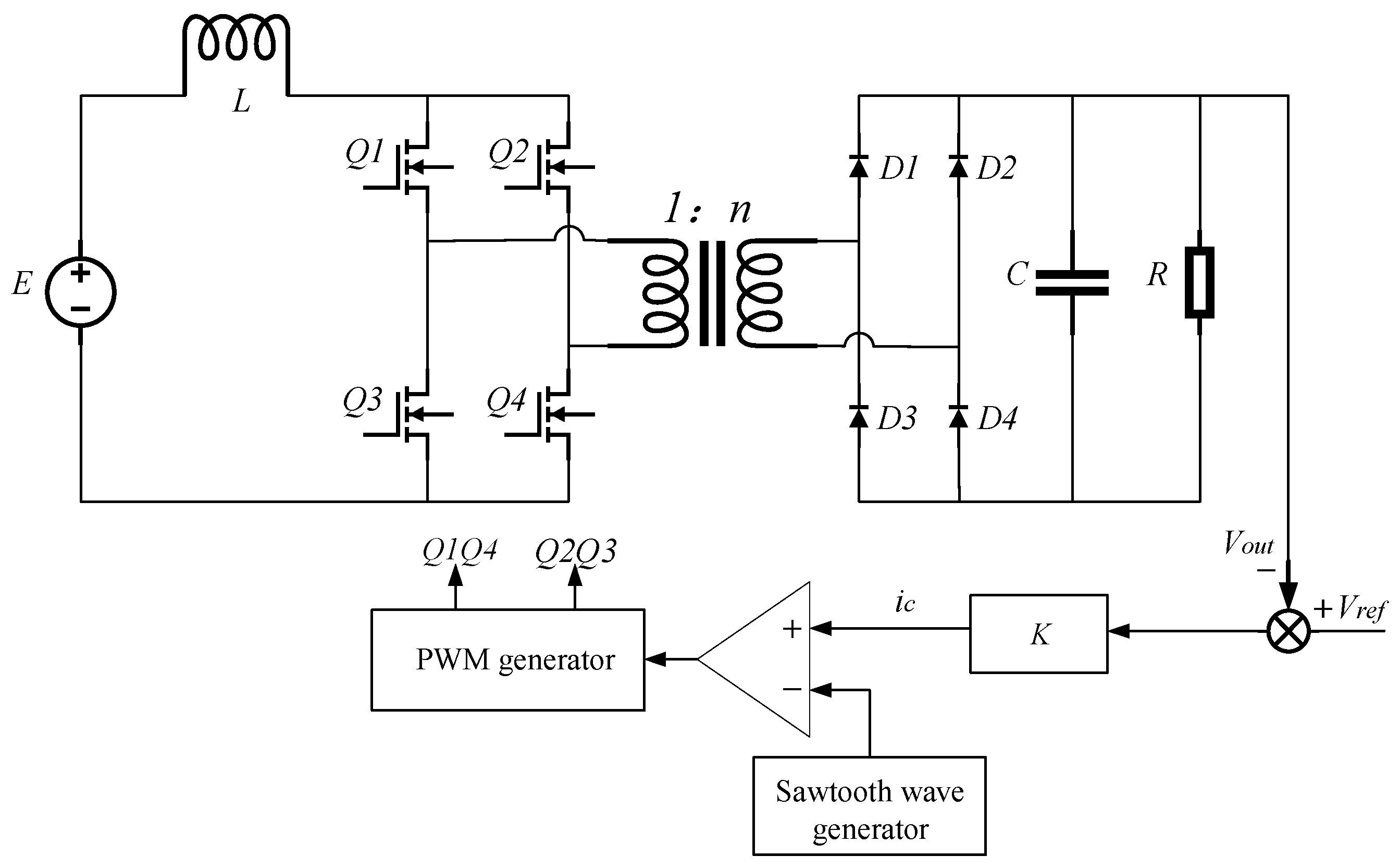
The schematic diagram of the system under voltage feedback control is shown in Figure 1. As can be seen from the figure, the system is a second-order circuit composed of an inductor and a capacitor. The operating principle of the circuit is as follows: The output voltage $V_{out}$ across the resistor $R$ is compared with the reference voltage $V_{ref}$, and the result is processed through the voltage feedback coefficient $K$, followed by a limiting adjustment, and the output signal i_c is obtained. Then, the signal is compared with the sawtooth wave to obtain the duty cycle $d_n$, and it is entered into the PWM generator. Then, the output signal from the PWM generator is made to control the switching states of the switches $Q_1$, $Q_2$, $Q_3$, and $Q_4$, where the signals for $Q_2$ and $Q_3$ are delayed by half a cycle relative to $Q_1$ and $Q_4$. The circuit has three states when the converter operates in DCM, as illustrated in Figure 2.

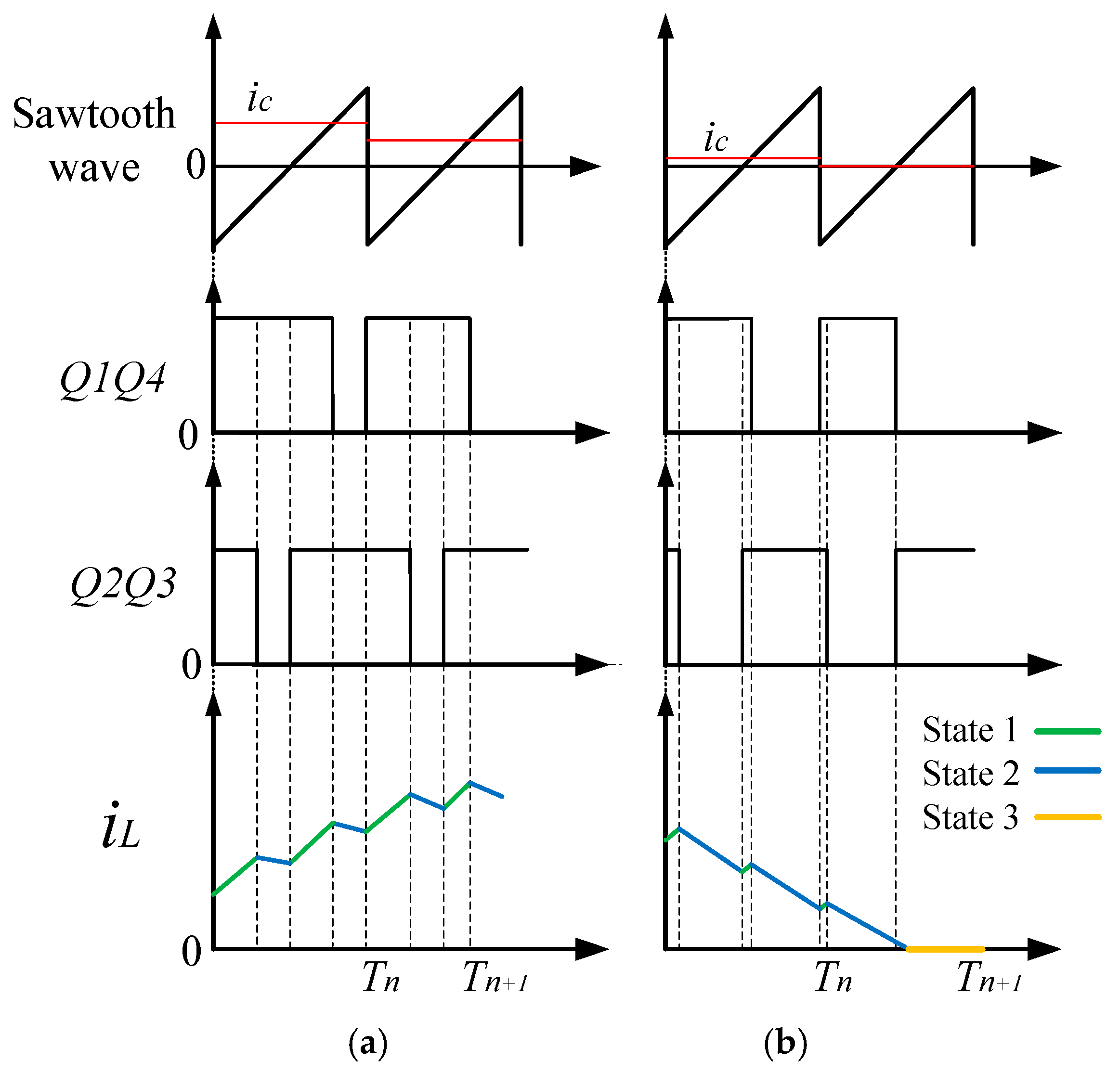
The duty cycle of the switches $Q_1$ and $Q_4$ in the n-th cycle is denoted as $d_n$, the duty cycle for State 1 is denoted as $d_1$, for State 2 as $d_2$, and for State 3 as $d_3$. When the circuit experiences only State 1 and State 2 during a complete cycle, its operating waveforms are shown in Figure 3a, and the duty cycle is expressed in Equation (1). Here, since the switches $Q_2$ and $Q_3$ lag behind switches $Q_1$ and $Q_4$ by half a cycle, the duty cycle of State 1 is $d_n-0.5$.

$$\left\{\begin{array}{c}{d}_1=d_n-0.5\hfill \\ d_2=1-d_n\hfill \end{array}\right.$$

(1)

When the circuit goes through all states during a complete cycle, its operating waveforms are shown in Figure 3b, and the duty cycle is expressed in Equation (2). The formula for $d_2$ is derived based on the inductance of the volt-second balance principle [16].

$$\left\{\begin{array}{l}{d}_1=d_n-0.5\\ d_2={\displaystyle \frac{E}{\frac{U_C\left(t\right)}{n_T}-E}}{d}_1\\ d_3=0.5-d_1-d_2\end{array}\right.$$

(2)

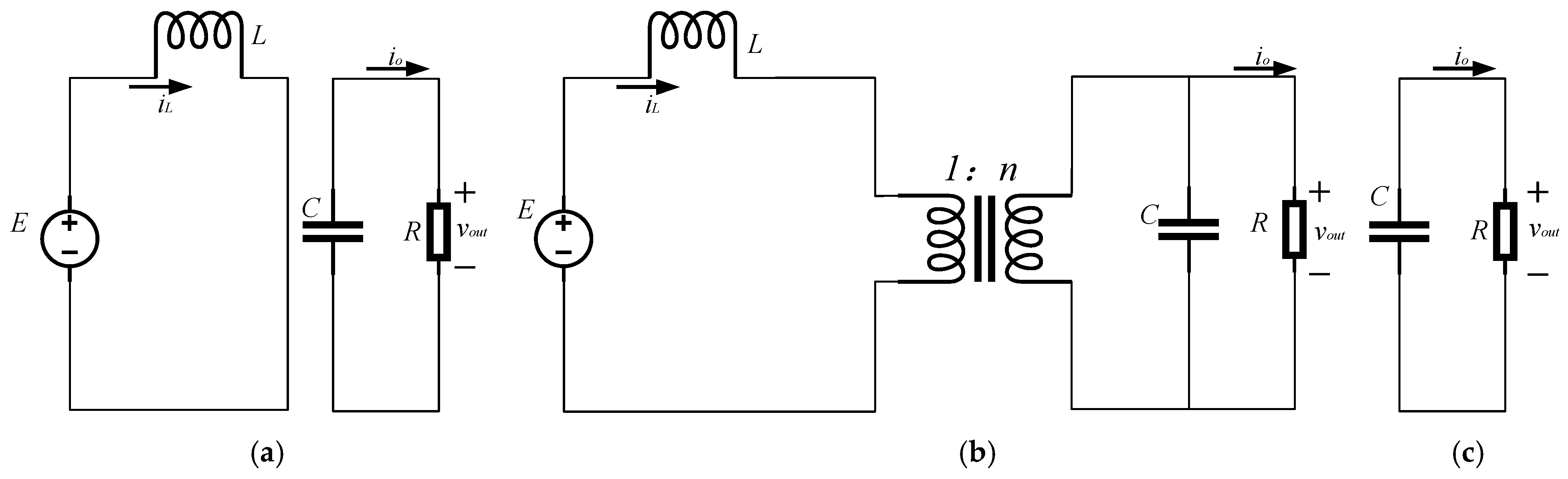
The first state is when switches $Q_1$, $Q_2$, $Q_3$, and $Q_4$ are on diodes; $D_1$, $D_2$, $D_3$, and $D_4$ are off; the inductor $L$ is charging, and the capacitor $C$ supplies energy to the load. The equivalent circuit is shown in Figure 2a, and the state equation at this time is given in Equation (3).

$$\left\{\begin{array}{ll}{\displaystyle \frac{\mathrm{d}{i}_L\left(t\right)}{\mathrm{d}t}}={\displaystyle \frac{E}{L}}& \left(nT<t\le \left(n+d_1\right)T\right)\\ {\displaystyle \frac{\mathrm{d}{U}_C\left(t\right)}{\mathrm{d}t}}=-{\displaystyle \frac{1}{CR}}{U}_C\left(t\right)& \left(nT<t\le \left(n+d_1\right)T\right)\end{array}\right.$$

(3)

The second state is when switches $Q_1$ and $Q_4$ are on, and $Q_2$ and $Q_3$ are off, and diodes $D_1$ and $D_4$ are on; $D_2$ and $D_3$ are off. Alternatively, switches $Q_2$ and $Q_3$ are on, and $Q_1$ and $Q_4$ are off, and diodes $D_2$ and $D_3$ are on; $D_1$ and $D_4$ are off. At this time, the inductor $L$ charges the capacitor $C$ and supplies energy to the load. The equivalent circuit is shown in Figure 2b, and the state equation at this time is given by Equation (4).

$$\left\{\begin{array}{ll}{\displaystyle \frac{\mathrm{d}{i}_L\left(t\right)}{\mathrm{d}t}}=-{\displaystyle \frac{1}{n_{T}L}}{U}_C\left(t\right)+{\displaystyle \frac{E}{L}}& \left(\left(n+d_1\right)T<t\le \left(n+d_2\right)T\right)\\ {\displaystyle \frac{\mathrm{d}{U}_C\left(t\right)}{\mathrm{d}t}}={\displaystyle \frac{1}{n_{T}C}}{i}_L\left(t\right)-{\displaystyle \frac{1}{CR}}{U}_C\left(t\right)& \left(\left(n+d_1\right)T<t\le \left(n+d_2\right)T\right)\end{array}\right.$$

(4)

The third state is when switches $Q_1$ and $Q_4$ are on; $Q_2$ and $Q_3$ are off, and all diodes are off, or switches $Q_2$ and $Q_3$ are on; $Q_1$ and $Q_4$ are off, and all diodes are off; the inductor $L$ continues to discharge to the secondary side, and the inductor current $I_L$ remains unchanged. However, since the diodes are off, only the capacitor $C$ provides energy to the load. The equivalent circuit is shown in Figure 2c, and the state equation at this time is given by Equation (5).

$$\left\{\begin{array}{ll}{\displaystyle \frac{\mathrm{d}{i}_L\left(t\right)}{\mathrm{d}t}}=0& \left(\left(n+d_2\right)T<t\le \left(n+d_3\right)T\right)\\ {\displaystyle \frac{\mathrm{d}{U}_C\left(t\right)}{\mathrm{d}t}}=-{\displaystyle \frac{1}{CR}}{U}_C\left(t\right)& \left(\left(n+d_2\right)T<t\le \left(n+d_3\right)T\right)\end{array}\right.$$

(5)

In line with frequency-domain mapping theory, half of the switching period T, denoted as Ts, is selected as the iteration period. Values of state variables from the n-th iteration cycle serve to calculate the values for the (n + 1)th cycle, enabling the derivation of the discrete iteration model of the converter’s primary circuit. The IBFBC operating in DCM has the following two operating trajectories:

$$\dot{x}={\left[\begin{array}{cc}{i}_L& U_C\end{array}\right]}^T$$

(6)

$$\begin{gathered} A_1=A_3=\left[\begin{array}{cc}0& 0\\ 0& -1/RC\end{array}\right], A_2=\left[\begin{array}{cc}0& -1/n_{T}L\\ 1/n_{T}C& -1/RC\end{array}\right] \\ {B}_1=B_2=\left[\begin{array}{c}{\displaystyle \frac{1}{L}}\\ 0\end{array}\right], B_3=\left[\begin{array}{c}0\\ 0\end{array}\right] \end{gathered}$$

(7)

When ($d_1$ + $d_2$)T = Ts, the converter operates in State 1 and State 2 within one sampling period. The discrete mapping model at the end of the n-th sampling period is given by Equation (8).

$$X_{n+1}=e^{A_2{d}_{2}T}{e}^{A_1{d}_{1}T}{X}_n+e^{A_2{d}_{2}T}{\int }_{nT}^{(n+d_1)T}{e}^{A_1\left(\left(n+d_1\right)T-\tau \right)}{B}_{1}Ed\tau +{\int }_{(n+d_1)T}^{(n+{\displaystyle \frac{1}{2}})T}{e}^{A_2((n+{\displaystyle \frac{1}{2}})T-\tau )}{B}_{2}Ed\tau$$

(8)

$e^{At}$ can be expanded using the series expansion of the matrix exponential function, as shown in Equation (9).

$${\mathrm{e}}^{At}=\mathit{I}+\mathit{A}t+{\displaystyle \frac{1}{2!}}{\mathit{A}}^2{t}^2+\cdots +{\displaystyle \frac{1}{n!}}{\mathit{A}}^n{t}^n+\cdots$$

(9)

When all eigenvalues of matrix $A$ have magnitudes less than 1, the higher-order terms in the above equation can be neglected for approximation [17].

When ($d_1$ + $d_2$)T < Ts, the converter operates in three states within one sampling period. The discrete mapping model at the end of the n-th sampling period is given by Equation (10).

$$\begin{array}{c}{X}_{n+1}=e^{A_3{d}_{3}T}{e}^{A_2{d}_{2}T}{e}^{A_1{d}_{1}T}{x}_n+e^{A_3{d}_{3}T}{e}^{A_2{d}_{2}T}{\int }_{(nT)}^{(n+d_1)T}{e}^{A_1((n+d_1)T-\tau )}{B}_{1}Ed\tau +e^{A_3{d}_{3}T}\\ {\int }_{\left(n+d_1\right)T}^{\left(n+d_2\right)T}{e}^{A_2((n+d_2)T-\tau )}{B}_{2}Ed\tau +{\int }_{\left(n+d_2\right)T}^{(n+{\displaystyle \frac{1}{2}})T}{e}^{A_3((n+{\displaystyle \frac{1}{2}})T-\tau )}{B}_{3}Ed\tau \end{array}$$

(10)

Equations (8) and (10) represent the discrete iterative mapping model of the IBFBC in DCM.

3. Analysis of the Dynamic Behavior of the Converter

The IBFBC has a specific stable operating region, and methods such as bifurcation diagrams, Poincaré sections, and Lyapunov exponents can be used to describe the chaotic evolution of the system. Among them, the bifurcation diagram method can specifically delineate the stable, bifurcation, and chaotic regions of the system’s operation; the Poincaré section determines whether chaos occurs by observing the intersection points, and the Lyapunov exponent identifies the boundary between stable and unstable regions. Additionally, fold diagrams can visually represent the stability of the system. The comprehensiveness and accuracy of the conclusions are enhanced by analyzing the converter’s dynamic behavior through multiple methods and cross-validating the results. This section investigates the effects of the voltage feedback coefficient K and input voltage E on the system’s performance using bifurcation diagrams, fold diagrams, Poincaré sections, and Lyapunov exponents.

The change in output voltage $V_{out}$ reflects the change in the operating state of the IBFBC. The main circuit parameters and the control system directly determine the system’s stability. The primary control parameter of the controller is the voltage feedback coefficient $K$. Therefore, the chaotic evolution of the system is studied by analyzing the variations in the output voltage $V_{out}$ caused by changes in the input voltage $E$ and the voltage feedback coefficient $K$, respectively.

Based on engineering experience, the circuit parameters are as follows: E = 100 V, K = 0.5, R = 160 Ω, C = 200 μF, L = 600 μH, fs = 15 kHz, V_ref = 400 V, and n_T = 1.

3.1. Bifurcation Diagram

The bifurcation diagram clearly illustrates how a nonlinear system transitions from a stable state to bifurcation and chaotic states as the bifurcation parameter changes. Using the discrete mathematical model of the system, an arbitrary initial value is selected for the iteration; the transient process is omitted, and the state variable samples at several fixed switching instants are retained. The sampled values under different bifurcation parameters are plotted to form the bifurcation diagram of the system [18].

When $K$ is used as the bifurcation parameter, E = 100 V, and when E is used as the bifurcation parameter, $K$ = 0.5, and the other parameters remain at the default settings. For parameters $K$ and E within the specified ranges, Equations (8) and (10) will be iterated multiple times to discard the initial transient results so that the system reaches a stable state. After stabilization, the output voltage $V_{out}$ is iterated and recorded continuously after each iteration, and the bifurcation diagrams with $K$ and E on the x-axis and output voltage $V_{out}$ on the y-axis are plotted separately. 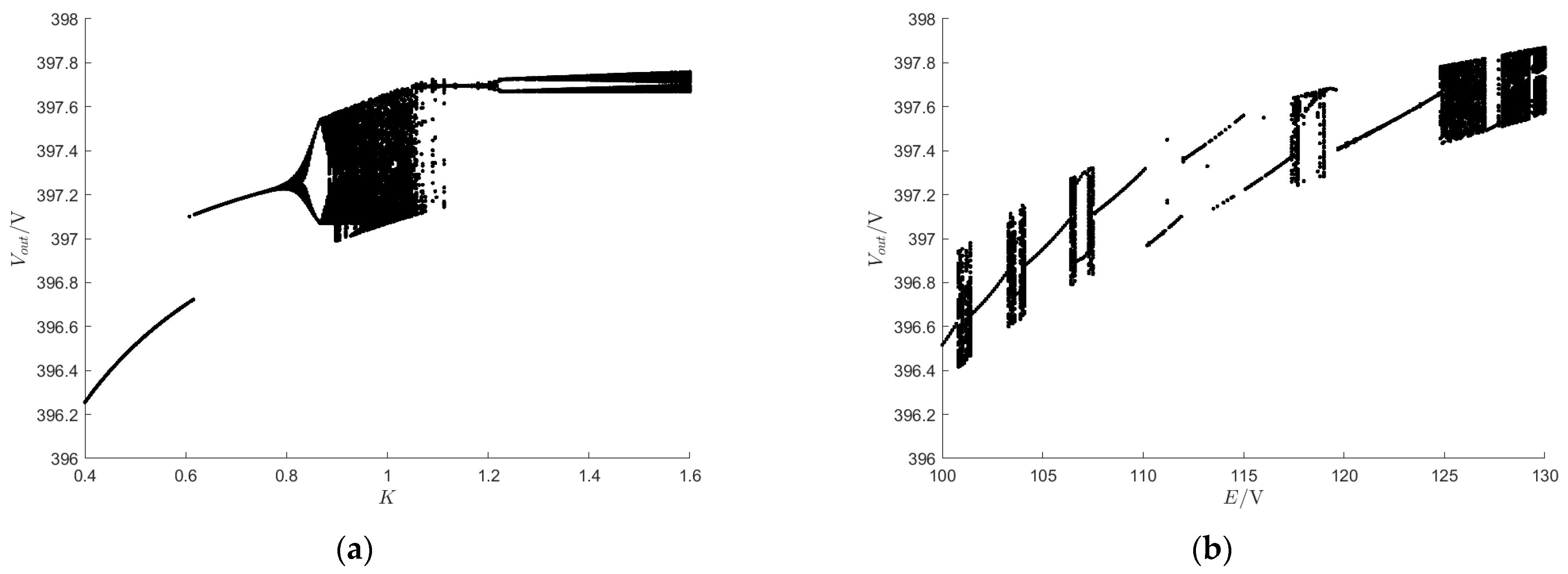The complexity and stability changes can be revealed by analyzing these diagrams in relation to the system’s dynamics across different $K$ and E values, providing profound insights into the system’s dynamical characteristics. The bifurcation diagram is shown in Figure 4.

Figure 4a shows that when K increases from 0.4 to 1.115 under this control mode, the system transitions from a stable state to an unstable chaotic state. Then, as $K$ increases from 1.115 to 1.175, the system oscillates between the unstable chaotic state and the stable state. Finally, when $K$ increases from 1.175 to 1.6, the system transitions to an unstable chaotic state through period-doubling bifurcation. The system operates stably when $K$ is between 0.4 and 0.75. Figure 4b shows that when the input voltage $E$ increases from 100 V to 130 V, the system repeatedly transitions from a stable state to an unstable chaotic state and back to a stable state before eventually entering an unstable chaotic state. In this chaotic regime, the system experiences deterioration in electrical energy quality, alongside increased thermal stress and voltage stress across the internal electronic components of the converter, thus resulting in a shortened converter lifespan and reduced energy conversion efficiency.

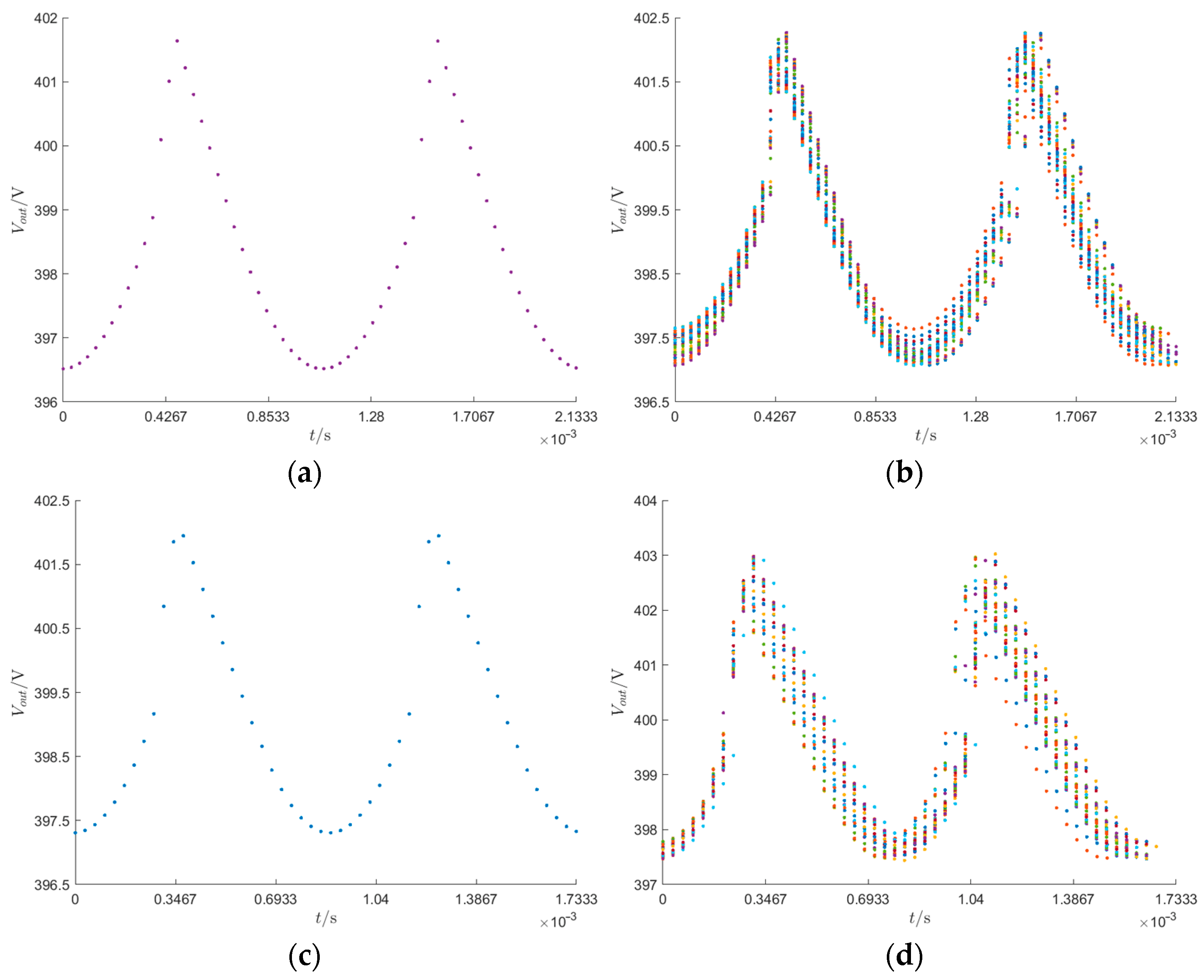
3.2. Fold Diagram

The fold diagram method can visually identify a system’s bifurcation and chaotic phenomena. The steps to plot a fold diagram are as follows: Firstly, an arbitrary initial value is selected and substituted into the discrete mathematical model for iteration. After the system stabilizes, the output values of several cycles are aligned and folded according to the sampling instants, resulting in the fold diagram [19]. Fold diagrams for 50 cycles are plotted by selecting $K$ = 0.5, $K$ = 1, $E$ = 110 V, and $E$ = 125 V, as shown in Figure 5.

In Figure 5a, when $k$ = 0.5, the output values of 50 cycles coincide with several sampling points, indicating that the system is stable. As shown in Figure 5b, when $k$ = 1, the fold diagram exhibits a dense distribution of sampling points, indicating that the system is in a chaotic state. In Figure 5c, when the input voltage $E$ is 110 V, the output values coincide with several sampling points, indicating that the system is stable. As shown in Figure 5d, when $E$ = 125 V, the fold diagram shows a dense distribution of sampling points, indicating that the system is in a chaotic state.

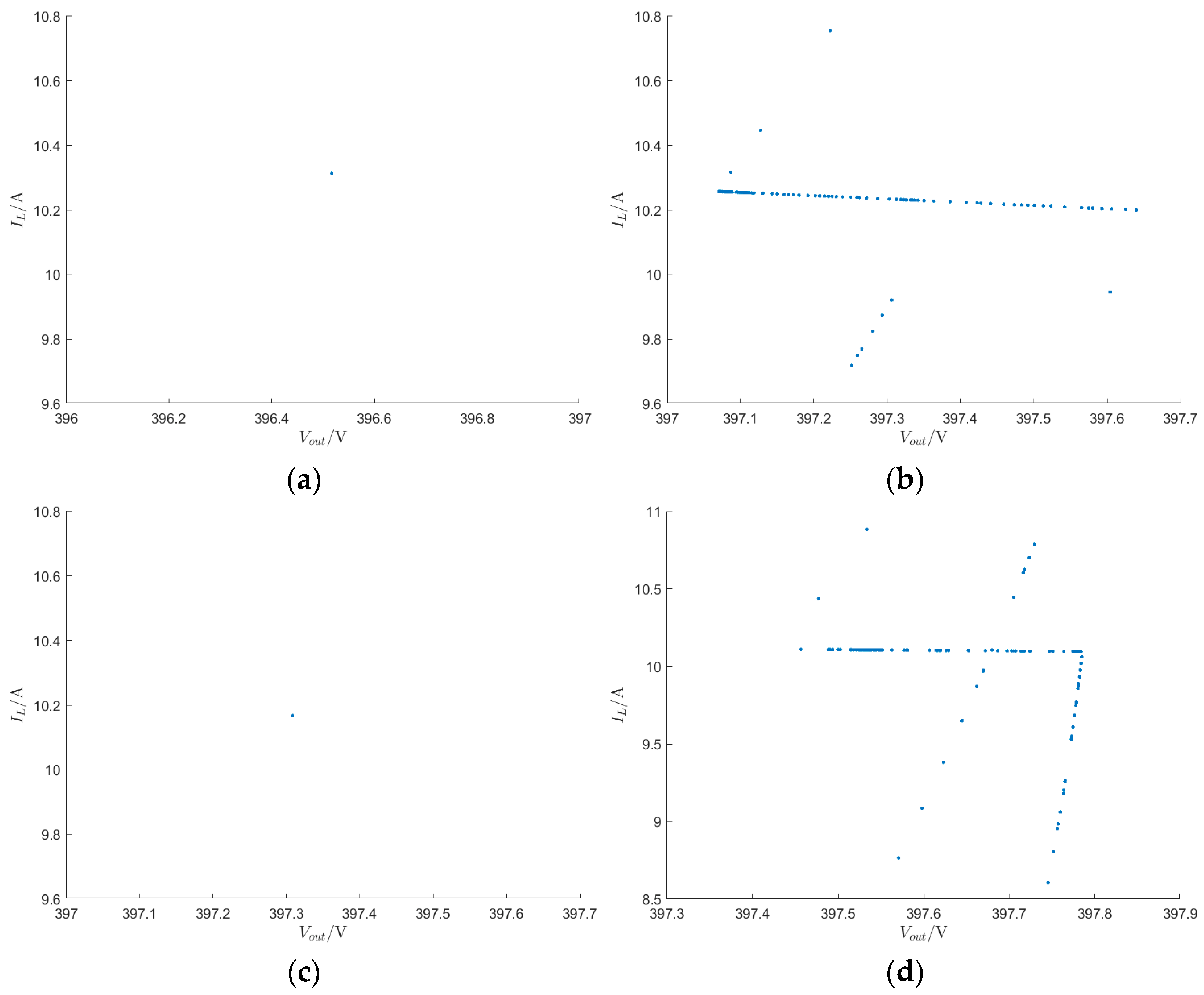
3.3. Poincaré Section

In phase space, a section is selected that neither tangentially intersects with the trajectory nor contains it, and this is known as the Poincaré section. The intersection points between the trajectory and the Poincaré section are called intersection points. According to the nonlinear dynamics theory, observing the pattern of the intersection points can determine whether chaos occurs; when there are only one or a few discrete points on the section, the motion is periodic, and the number of points represents the period of the state; when the intersection points form a closed curve, the motion is quasi-periodic; and when the intersection points form a dense region or exhibit a fractal structure, the system is in a chaotic state [20].

This section begins with the state equations for different operating modes to demonstrate that the converter exhibits the rich nonlinear behavior shown in the bifurcation diagram of Figure 4 as the voltage feedback coefficient K and input voltage E increase. The Runge–Kutta algorithm is used to directly solve the differential equations within each switching cycle, resulting in the Poincaré sections of the IBFBC at $K$ = 0.5, $K$ = 1, $E$ = 110 V, and $E$ = 125 V, as shown in Figure 6.

As shown in Figure 6a, it is clear that when $K$ = 0.5, the points on the Poincaré section are discrete. Based on the number of points, it can be determined that the converter operates in period-1. In Figure 6b, the intersection points have formed clusters in certain regions, indicating that when $K$ = 1, the converter operates in a chaotic state. In Figure 6c, when $E$ = 110 V, the points on the Poincaré section are discrete, with only one point, indicating that the converter operates in period-1. In Figure 6d, the intersection points have formed clusters in certain regions, indicating that when $E$ = 125 V, the converter operates in a chaotic state. These results are consistent with the states presented at each point in the bifurcation diagram in Figure 4, confirming the correctness of the discrete mapping model and providing a more intuitive representation of the operating state of the converter as the voltage feedback coefficient $K$ and input voltage $E$ take on different values.

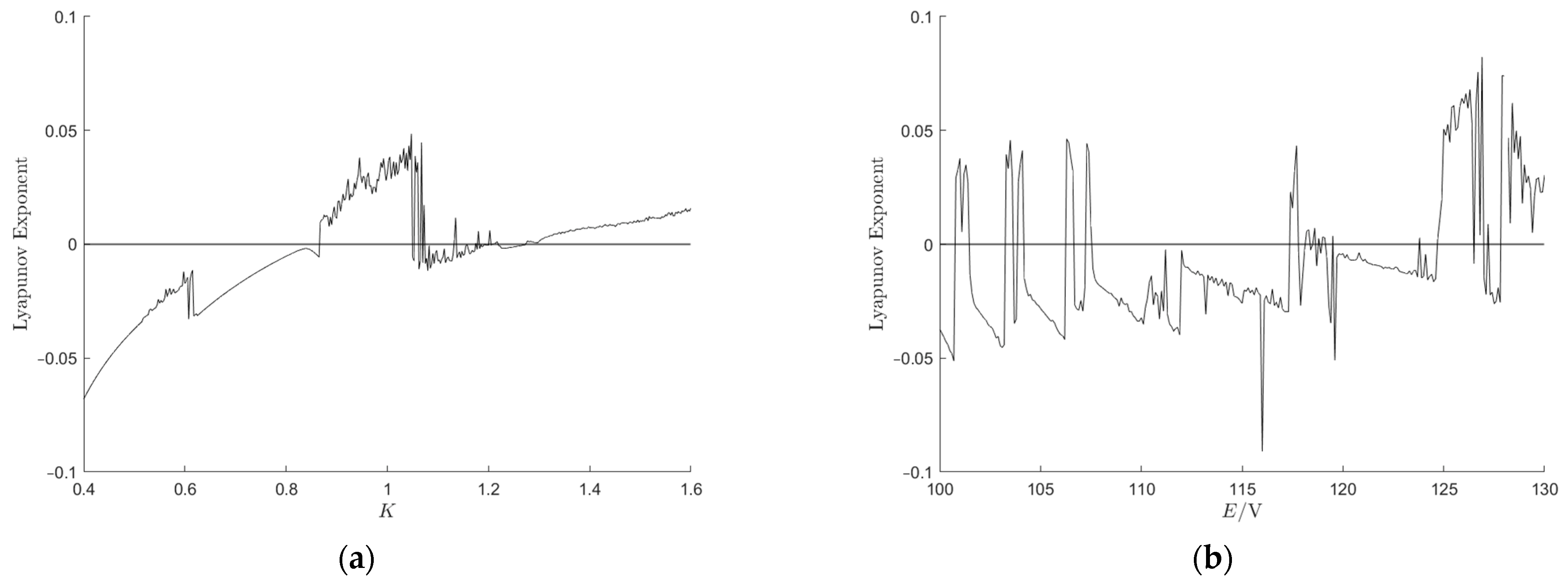
3.4. Lyapunov Exponent

The Lyapunov exponent quantitatively describes the degree to which two trajectories, originating from two infinitesimally close initial values, converge or diverge exponentially after undergoing iterations and evolving over time. It serves as a measure of the system’s dynamical characteristics. It characterizes the average exponential rate at which the distance between neighboring trajectories in the system either converges or diverges in phase space. Lyapunov exponent less than zero indicates that neighboring points converge to a single point after multiple iterations, meaning that the system is stable. Lyapunov exponent greater than zero indicates that two neighboring points eventually separate exponentially, meaning that the system is unstable. Lyapunov exponent equal to zero corresponds to the boundary between stability and instability [21].

For a two-dimensional mapping $x_{n+1}=f\left(x_n\right)$, where $x$ is the state vector ${\left[\begin{array}{cc}{i}_L& U_C\end{array}\right]}^T$, the Lyapunov exponent (LE) can be calculated using the Benettin method. Two initially close vectors $x_0$ and $x_0^{\prime }$ are selected, with their initial distance defined as ${\delta }_0=\parallel x_0^{\prime }-x_0\parallel$. Through multiple iterations of the mapping, the deviation at each step is recorded as ${\delta }_n=\parallel x_n^{\prime }-x_n\parallel$. The Lyapunov exponent is then defined by Equation (11).

$$LE=\underset{n\to \infty }{\lim }{\displaystyle \frac{1}{n}}\sum _{i=0}^{n-1}\ln \left({\displaystyle \frac{{\delta }_{i+1}}{{\delta }_i}}\right)$$

(11)

Using Equation (11), the Lyapunov exponent of the system can be calculated when the voltage feedback coefficient $K$ and input voltage $E$ are varied. The resulting Lyapunov exponent plots are shown in Figure 7.

From Figure 7a, it can be seen that when 0.4 ≤ $K$ < 0.75, the Lyapunov exponent is less than zero, indicating that the system is in a stable state. When 0.75 ≤ $K$ < 0.865, the Lyapunov exponent initially increases, approaches zero, and then decreases, indicating that the system undergoes period-doubling bifurcation. When 0.865 ≤ $K$ < 1.115, the system enters a chaotic state. When 1.115 ≤ $K$ < 1.175, the system exhibits transitions between unstable chaotic states and stable states. For $K$ ≥ 1.175, the system enters a chaotic state through period-doubling bifurcation. Figure 7b shows that as the input voltage $E$ increases from 100 V to 130 V, the system repeatedly transitions from a stable state to an unstable chaotic state and then back to a stable state, ultimately settling into an unstable chaotic state. The Lyapunov exponent results are consistent with those obtained from the bifurcation diagrams.

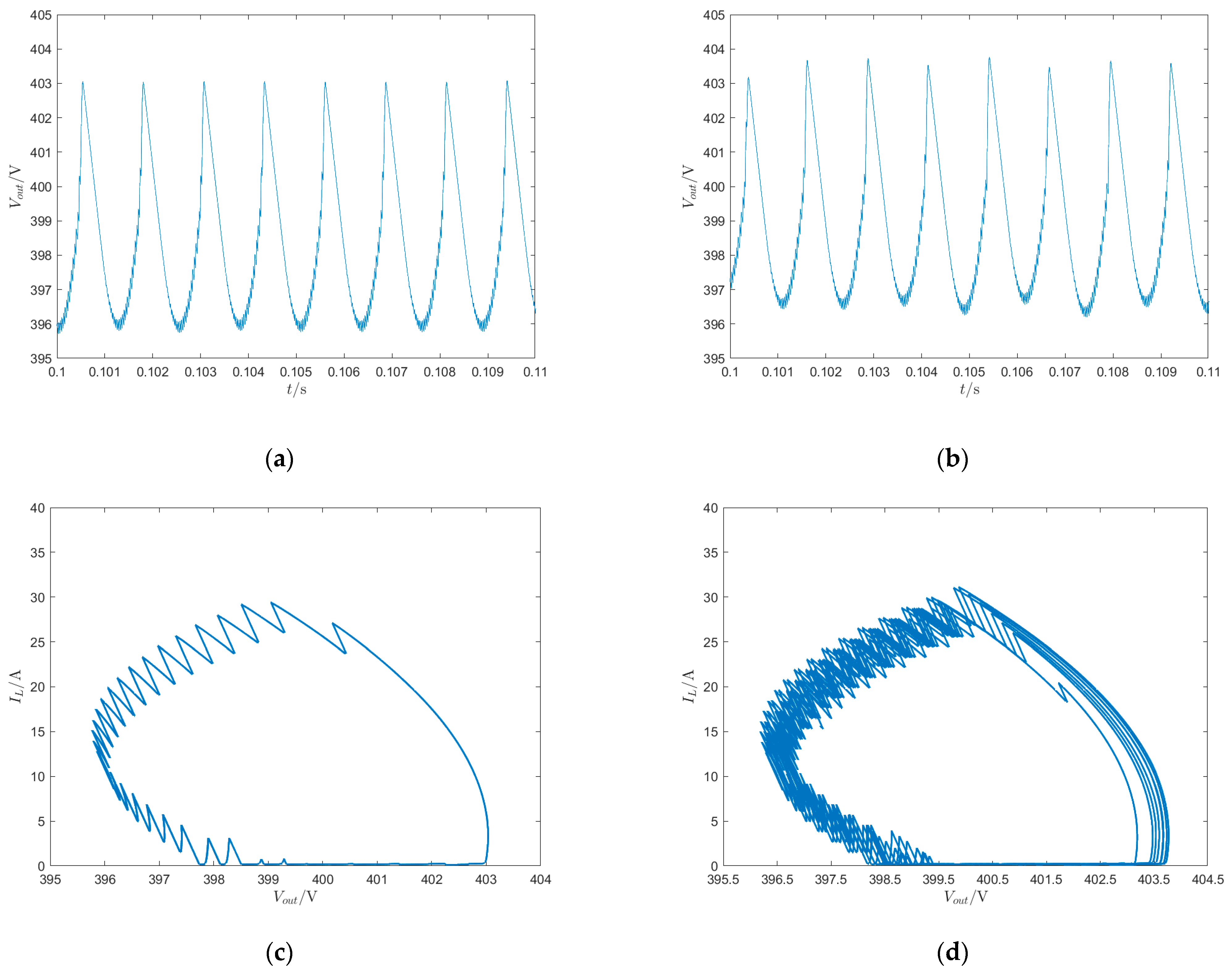
4. Simulation Verification

Based on the circuit schematic in Figure 1 of Section 2, a simulation model was constructed in the MATLAB R2022a/Simulink environment. Building on the analysis in Section 3, different voltage feedback coefficients $K$ and input voltages $E$ that lead to either system stability or chaos were selected, while other circuit parameters remain consistent with those described in Section 3. The simulation results for $K$ = 0.5 and $K$ = 1 are shown in Figure 8.

Figure 8 shows the time-domain waveform for different Ks. Figure 8a,c show that when the voltage feedback coefficient $K$ is 0.5, the time-domain waveform is periodic, and the phase trajectory diagram consists of a single, closed curve. From the time-domain waveform of $I_L$, it is evident that the converter is indeed operating in DCM under the given circuit parameters. Figure 8b,d show the time-domain waveform and phase trajectory diagram when the voltage feedback coefficient $K$ = 1. At this point, the converter operates in a chaotic state, with the time-domain waveform losing periodicity and appearing erratic, displaying large amplitude jumps between switching cycles. This indicates that the chaotic state is unstable and detrimental. The phase trajectory diagram consists of trajectories randomly distributed within a certain region.

The simulation results for $E$ = 110 V and $E$ = 125 V are shown in Figure 9.

Figure 9 shows the time-domain waveform for different Es. As shown in Figure 9a,c, when the input voltage is 110 V, the time-domain waveform is periodic, and the phase trajectory diagram consists of a single, closed curve, indicating that the system is in a stable state. Figure 9b,d show the time-domain waveform and phase trajectory diagram when the input voltage is 125 V. At this point, the converter operates in a chaotic state, with the time-domain waveform losing periodicity and appearing erratic, displaying large amplitude jumps between switching cycles. The phase trajectory diagram consists of trajectories randomly distributed within a certain region.

It is evident from the simulation results that the phenomena observed in the time-domain waveforms and phase trajectory diagrams obtained through simulations are fully consistent with conclusions drawn from various previous nonlinear methods. When the simulation results are stable, the corresponding bifurcation diagrams, folding diagrams, and Poincaré sections are stable, and the Lyapunov exponent is less than zero. In chaotic states, the corresponding bifurcation diagrams, folding diagrams, and Poincaré sections are also chaotic, and the Lyapunov exponent is greater than zero. These results confirm the discrete iteration model’s correctness and enhance the conclusions’ persuasiveness and credibility.

5. Discussion and Analysis

Through this study, a comprehensive analysis of the nonlinear dynamic behavior of IBFBC was conducted, and the correctness of the model was verified. The following discussion will focus on three aspects: in-depth analysis of the research findings, comparison with existing studies, and implications for engineering applications.

5.1. In-Depth Analysis of Research Findings

Through the comparative analysis of bifurcation diagrams, fold maps, Poincaré sections, and Lyapunov exponents, it is evident that the bifurcation and stability regions obtained using different methods are nearly identical. This consistency demonstrates that the constructed discrete iterative model accurately captures the nonlinear dynamic behavior of IBFBC under voltage feedback control. Furthermore, the results confirm that as the voltage feedback coefficient $K$ and input voltage $E$ vary, the IBFBC system undergoes dynamic evolution through multiple states, including stability, bifurcation, and chaos. Additionally, the simulation results align perfectly with the conclusions drawn from various nonlinear methods, further validating the accuracy and applicability of the proposed model. Notably, the model’s precise prediction of chaotic states and stability regions provides a solid theoretical foundation for the development of subsequent control strategies. The specific descriptions of the nonlinear dynamic behaviors when the voltage feedback coefficient $K$ is the variable are as follows: when 0.4 ≤ $K$ < 0.75, the system remains in a stable state; when 0.75 ≤ $K$ < 0.865, the system undergoes period-doubling bifurcation; when 0.865 ≤ $K$ < 1.115, the system enters a chaotic state; when 1.115 ≤ $K$ < 1.175, the system alternates between unstable chaotic and stable states; when $K$ ≥ 1.175, the system transitions to an unstable chaotic state through period-doubling bifurcation. When the input voltage is the variable such as when the input voltage $E$ increases from 100 V to 130 V, the system repeatedly transitions from a stable state to an unstable chaotic state and back to a stable state, eventually settling into an unstable chaotic state.

5.2. Comparison with Existing Studies

Compared to previous studies, this paper not only delves deep into the influence of nonlinear dynamic behaviors on the IBFBC system but also verifies the consistency of the results through multiple nonlinear analysis tools, such as Lyapunov exponents and Poincaré sections. Unlike traditional models, the discrete iterative model proposed in this study demonstrates higher precision and reliability in both mathematical derivation and simulation validation. Moreover, it is better suited for analyzing nonlinear dynamic behaviors, providing a more robust foundation to understand and optimize the IBFBC system.

5.3. Implications for Engineering Applications

The discrete iterative model derived in this study, along with the identified nonlinear dynamic behaviors, provides valuable guidance and a reference for the selection of input voltage and the design of the voltage feedback coefficient in IBFBC systems. In DCM voltage-Fed IBFBC, for the same parameters, the voltage feedback coefficient $K$ should be within the range of 0.4 to 0.75, while the input voltage $E$ should be within the ranges of 108 V to 117 V and 120 V to 125 V to ensure that the system remains in a stable state. When the actual parameters exceed the above-mentioned ranges, chaos control methods, such as the exponential delayed feedback chaos control method or the resonant parametric perturbation method, can be employed. These methods can modify PWM control to mitigate the impact of nonlinear dynamic behaviors and help restore system stability.

IBFBC is widely used in fields such as fuel cells and electric vehicles. Fuel cells typically have low output voltage and are highly susceptible to load fluctuations, necessitating the use of IBFBC to address challenges such as high boost ratios, wide input voltage ranges, high efficiency, and electrical isolation. By appropriately adjusting certain circuit or control loop parameters based on the results of this study, the impact of nonlinear dynamic behaviors can be effectively mitigated, thereby extending the converter’s lifespan and reducing energy losses. The findings of this study provide a theoretical foundation for improving the adaptability of IBFBC under complex operating conditions and offer valuable insights for further research in related fields.

6. Conclusions

This paper investigates the nonlinear behavior of the isolated boost full-bridge converter (IBFBC) in DCM. Based on an analysis of the circuit’s operating principle, a discrete iterative model of the system is established. Using this model, bifurcation diagrams under varying parameters are plotted, revealing that the system eventually enters a chaotic state as the control and circuit parameters change. Fold diagrams and Poincaré sections are then employed to visually demonstrate the stable and chaotic states of the system under different control and circuit parameters. The Lyapunov exponent method is used to determine these parameters’ influence on the system’s dynamic characteristics. Finally, a simulation model is constructed in MATLAB R2022a/Simulink, where the rich dynamic evolution of the converter is observed through time-domain and phase trajectory diagrams under various parameter changes, further validating the discrete mapping model. The results of this study provide valuable guidance and a reference for the selection of circuit parameters and the design of controllers for the IBFBC.

Despite the effectiveness of the proposed discrete iterative model in describing the nonlinear behavior of IBFBC, certain limitations remain. The model employs a simple proportional feedback control, which results in relatively large voltage ripples and less distinct experimental results than expected. The varying parameters did not account for the influence of other factors, such as inductance and capacitance values, which restricts the applicability of this study. Future research can address these limitations through the following improvements: we plan to incorporate more parameters and improve the control strategy, such as adding an integral component, to enhance the generality of the experimental results and reduce the impact of voltage ripple on the result analysis.