Smart Spectrum Recommendation Approach with Edge Learning for 5G and Beyond Radio Planning

Abstract

Radio spectrum planning has become increasingly important, since the radio spectrum is a scarce resource. Moreover, the utilization of millimeter wave (mmWave) frequencies with fifth-generation (5G) standards has made radio planning more compelling. Considering their different strengths and weaknesses, it is essential to know when mmWave frequencies should be selected in radio planning. In this paper, an approach with edge learning is developed to provide smart spectrum recommendations on which frequency bands should be used for a region. Using the proposed approach, radio spectrum planning can be carried out more efficiently, especially for the frequency ranges of mmWave communications. The proposed approach is designed with a distributed structure, based on awareness of the environment and ambient intelligence. This approach can be performed for each transmission point considering the environment information of the related coverage area. As a result, radio spectrum planning can be conducted for an entire region with the proposed system. The results show that this study both enhances overall user satisfaction and provides reasonable recommendations to operators in the transition to mmWave usage. Thus, the developed approach can be utilized for 5G and beyond communications. Specifically, this methodology is based on applying supervised ML algorithms to a synthetically generated dataset, and the best model achieves around 80% classification accuracy, demonstrating the feasibility of the approach. These quantitative results confirm its practicality and provide a concrete baseline for future studies.

1. Introduction

The utilization of the radio spectrum increases over time with the extensive use of wireless communication systems [1]. Thus, the use of higher frequencies than existing ones has become increasingly important for next-generation communication systems [1,2,3]. As an example, fifth-generation (5G) wireless standards have been developed to enable the use of frequencies up to 71 GHz [4]. The potential challenge of using higher frequencies becomes more apparent in sixth-generation (6G) networks [5,6,7,8].

While 5G millimeter wave systems exhibit both strengths (large bandwidths and directional beams) and weaknesses (blockage sensitivity and high penetration loss), these aspects have been sufficiently studied in previous works [9]; thus, the focus of this study is on the implications for practical spectrum planning. From a practical perspective, it is necessary to determine when mmWave systems should be deployed in a region, considering the adopted radio planning approach.

There are two main frequency ranges (FRs); these are defined in 3GPP standardization as FR1 and FR2 [4]. FR1 includes microwave frequencies, and FR2 consists of two sub-bands (FR2-1 and FR2-2) for mmWave frequencies. In this study, an environment-aware approach with ambient intelligence is developed to provide smart spectrum recommendations for selecting the appropriate FR for a transmission point (TP). 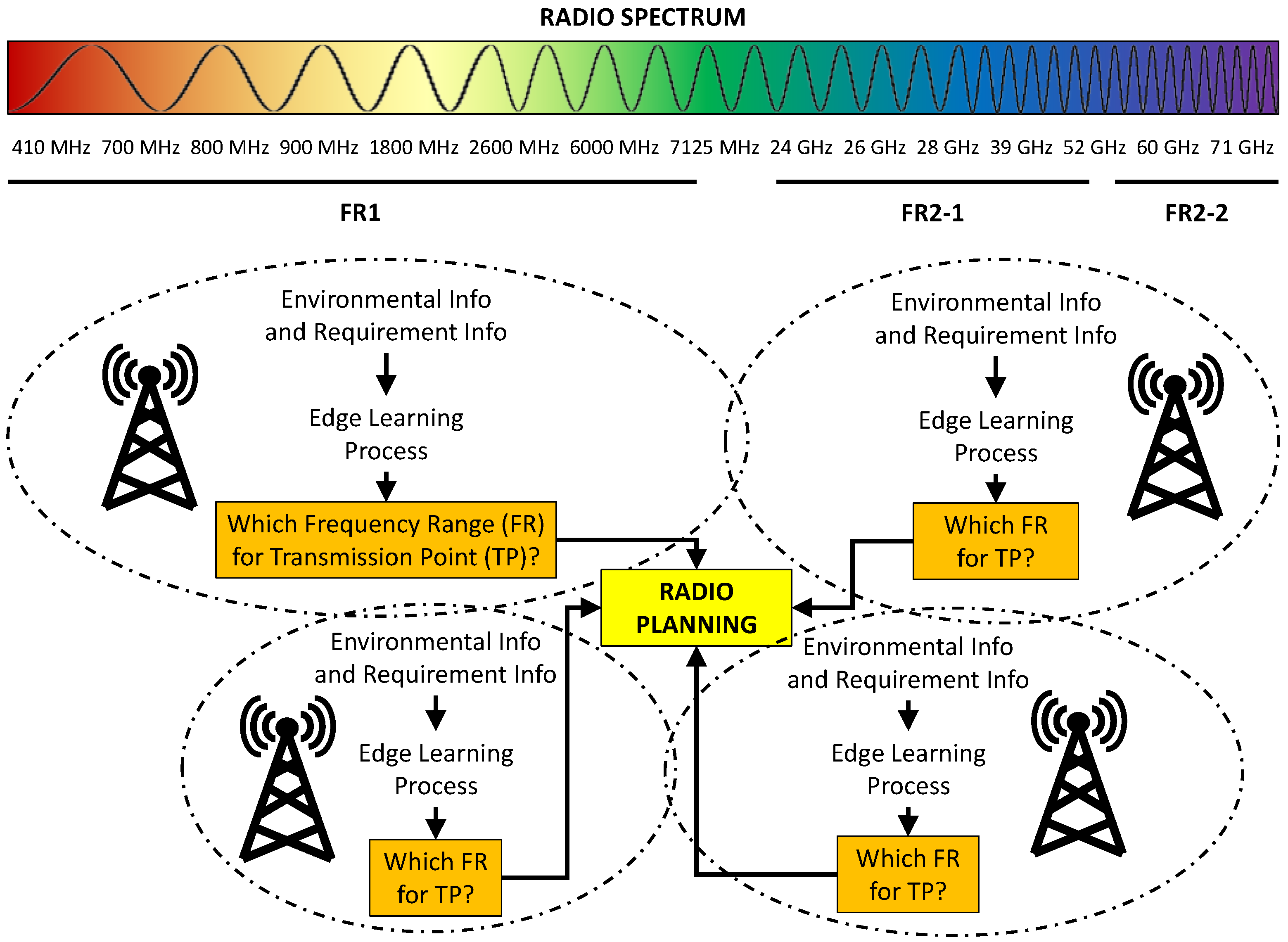Thus, Figure 1 shows the general definition of the problem. In the proposed approach, environmental information and user-specific requirement information feed the decision mechanisms under the transmission points.

This approach is designed to determine which FR should be used for a TP considering environment awareness and user-specific requirements. This part of the study operates in a distributed structure for each TP region (edge). In the next part, general radio planning is conducted for a whole region using the decisions of each TP region. In other words, there are two cascaded structures under the proposed approach: (1) FR group decisions at the edges (for each TP); (2) ultimate centralized decisions for different TPs under a whole region. The proposed approach aims to estimate new TP needs during the 5G transition for a region or to find out new TP locations for a new coverage region. Thus, the person conducting radio planning can analyze the whole region for full coverage with the subregions.

Existing research in this field can be grouped into three categories: (i) mmWave channel modeling, (ii) spectrum planning and optimization, and (iii) machine learning (ML)-based approaches.

For the first group, there are several studies on coverage and wireless channel characteristics considering the mmWave frequency bands [10,11,12,13]. In [10], the mmWave coverage and channel characteristics are analyzed using ray tracing methods. Channel models and design considerations are investigated for mmWave communications in [11]. A comprehensive indoor propagation measurement and channel modeling study at 6.75 GHz and 16.95 GHz in mid-band spectrum is conducted in [12]. The behavior of 60 GHz mmWave power transmission under outdoor snowstorm settings is investigated in [13].

There are also studies on cellular network planning and optimization [14,15,16,17,18,19,20,21]. A particular study highlights cutting-edge modeling and radio planning approaches that leverage stochastic geometry and Monte Carlo simulations for millimeter-wave (mmWave) frequency bands [14]. In [15], the cellular network planning issue in the context of heterogeneous networking is discussed from different perspectives. A three-dimensional dense network planning method to deploy small base stations with mmWave frequencies is proposed in [16]. Ref. [17] proposes a base station clustering framework utilizing unsupervised learning techniques to delineate optimal target areas for 5G network deployment. A multi-objective optimization algorithm that considers the main constraints of coverage, capacity, and cost for high-capacity scenarios that range from dense to ultra-dense mmWave 5G standalone small-cell network deployments is studied in [18]. An efficient implementation of a 3GPP three-dimensional (3D) channel model with the goal of minimizing the computational time required for channel simulation is proposed [19].

Moreover, 5G mmWave network planning using ML techniques for path loss estimation is studied in [20]. Lastly, [21] enhances mmWave channel estimation for network planning using deep learning (DL).

The proposed environment-aware and ambient intelligence-based approach introduces the following contributions, which distinguish it from prior work. Unlike previous studies that apply ML only for narrow optimization tasks, our contributions demonstrate novelty through (a) employing synthetic data generation for improved robustness, and (b) linking spectrum planning objectives directly with quantifiable mmWave propagation characteristics.

• A reference approach and method are proposed for comparative evaluation of similar smart spectrum recommendation studies with edge learning for 5G and beyond radio planning including mmWave frequencies.
• Environmental information and user-specific information are associated with the given problem definition for radio planning.
• To facilitate ML applications, a new synthetic dataset has been generated, integrating data on environmental influences and individual user needs. The features are associated with channel properties.
• Using the synthetic tabular dataset, optimal hyperparameter settings are determined for a range of ML algorithms, encompassing traditional learning models, ensemble approaches, and neural networks (NNs).

The remainder of this paper is organized as follows. Section 2 outlines the fundamental concepts of the radio spectrum relevant to 5G standardization and the basics of mmWave communication. Section 3 details the proposed methodology. Section 4 presents the outcomes of the ML classification algorithms, including hyperparameter tuning results and case studies with comparative analyses. Finally, Section 5 concludes the paper and highlights several open research challenges.

2. Preliminaries

This section provides a brief overview of the fundamentals of the radio spectrum for 5G New Radio (NR) standardization and mmWave communication, closely related to the proposed approach.

2.1. Radio Spectrum for 5G Standardization

The radio spectrum is limited by the available frequency bands, even though it is a natural and inexhaustible resource. This limitation makes the radio spectrum crucial in the field of communication. The radio spectrum usually includes frequencies between 30 Hz and 300 GHz. Currently, there is significant focus on the development and research in beyond-5G communication, where higher frequency ranges become increasingly important.

Under the available 3GPP standardization, 5G operates in a variety of FRs including FR1, FR2-1, and FR2-2 [4]. FR1 frequencies provide the integration of 5G into available cellular networks thanks to its wide coverage area and existing infrastructure compatibility, while FR2 frequencies enable high-capacity data transmission in the regions with high user traffic and large bandwidth requirements thanks to the mmWave communication capabilities.

As shown in

Table 1. The frequency ranges in 5G standards.

Frequency Range (FR)	Upper and Lower Bounds	Example 5G Frequency Bands
FR1	410–7125 MHz	410 MHz, 700 MHz, 800 MHz, 900 MHz, 1800 MHz, 2600 MHz, 6000 MHz, 7125 MHz
FR2-1	24.25–52.60 GHz	24 GHz, 26 GHz, 28 GHz, 39 GHz, 52 GHz
FR2-2	52.60–71.00 GHz	52 GHz, 60 GHz, 71 GHz

, FR1 covers the frequency bands between 410 MHz and 7125 MHz [22]. FR1 is also known as sub-6GHz and it is mostly compatible with existing Long-Term Evolution (LTE) infrastructures. On the other hand, FR2 is divided into FR2-1 (24,250–52,600 MHz) and FR2-2 (52,600–71,000 MHz). These mmWave frequency bands are generally planned to be used in the regions with high data rates and large bandwidths, especially for dense networks with small-cell deployments.

2.2. Millimeter Wave Communication

The mmWave frequencies such as 24 GHz, 26 GHz, 28 GHz, 39 GHz, 52 GHz, 60 GHz, and 71 GHz are an ideal option in densely populated areas with heavy data traffic [23]. From the perspective of frequency utilization, 5G NR leverages mmWave frequencies to enhance wireless communication systems. Frequency bands of mmWave offer high bandwidth capabilities while providing promising solutions in terms of efficiency and timing, demonstrating potential for substantial advancements in performance and capacity.

On the contrary, mmWave frequency bands have several important challenges related to wireless channel properties. One of the primary challenges is the high path loss due to the shorter wavelength. This results in reduced signal coverage and limits the communication range. Additionally, mmWave attenuation caused by wind and heavy rain impacts the link budget.

As another challenge, mmWave signals are more susceptible to obstructions. Hence, mmWave communication faces challenges from obstacles such as buildings, which can lead to coverage gaps, especially in urban environments. Shadowing effects further complicate signal reliability.

In addition to the path loss and shadowing properties of the wireless channel, fading due to multipath propagation can degrade signal quality in mmWave communication. As mmWave signals are highly sensitive to scattering and reflections, they experience particularly significant multipath effects. Moreover, Doppler effects are critical due to the small wavelength and high mobility.

mmWave communication holds great potential for high-speed wireless connectivity, but it comes with a set of challenges related to path loss, blockage, and multipath propagation.

3. Methods and Materials

This section defines the research objectives, problems, and methodology. The research objective of the study is to design a smart spectrum recommendation approach that decides on the most appropriate FR group (FR1, FR2-1, or FR2-2) for each transmission point during 5G and beyond planning. Then, the research problem deals with how to utilize environmental and user-specific information effectively for FR group recommendation. Some of the sub-problems can be listed as (i) establishing the link between environment/user features and spectrum decisions, (ii) generating synthetic datasets that reflect realistic wireless channel conditions, and (iii) designing ML-based decision mechanisms at the edge. As a research methodology, supervised ML algorithms are applied on a synthetically generated dataset derived from channel models. Moreover, the following tools are employed in the study: dataset generation via MATLAB 2023b; ML model training using scikit-learn and Orange Data Mining; evaluation through accuracy, F1-score, and extended metrics (per-class precision).

A general block diagram for the proposed approach is given in Figure 2. At the edges (TPs), information is collected via geographic information system (GIS) and TP, including geographic characteristics, residential area plans, general weather conditions, vehicle traffic density, user density, indoor/outdoor usage, and IoT system density. This information is processed at the edges to determine FR selection (FR1, FR2-1, or FR2-2) for the TP region. ML algorithms are employed to support decision-making at the edges. After that, each edge decision is gathered to complete radio planning for the whole region.

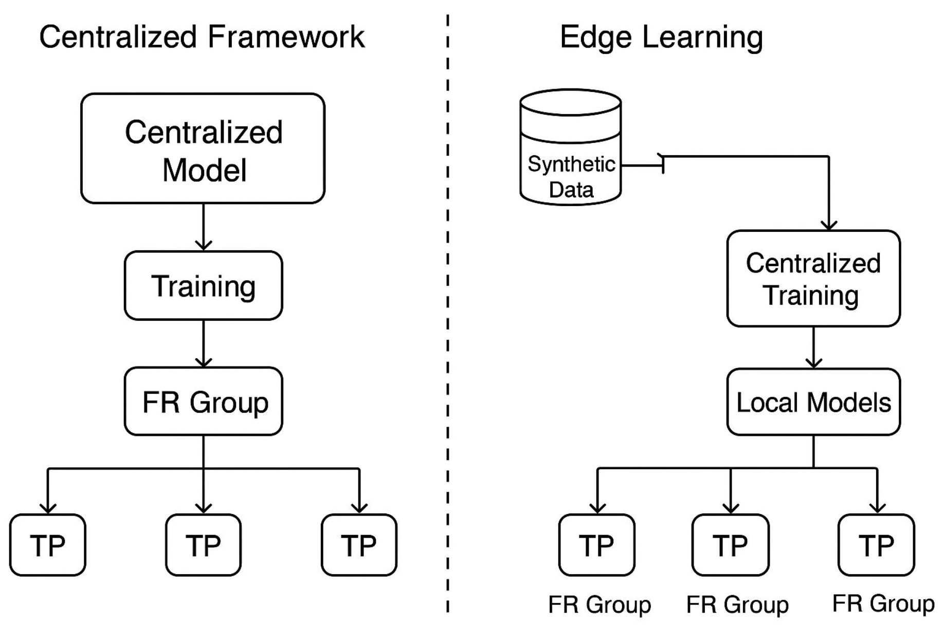
The proposed framework adopts an “edge learning” paradigm. At each transmission point (edge), a local ML model performs inference to decide the optimal FR group. Training is initially centralized using synthetic data but models can be updated at the edge through periodic re-training using locally available information. The distributed edge-based decisions differ from a centralized model in that each TP autonomously adapts to its local environment while still contributing to a regional aggregation stage. 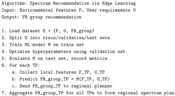Figure 3 illustrates this architecture. The pseudocode of the main algorithm is provided below:

In the absence of publicly available datasets relevant to the specified problem, we develop a synthetic dataset to enable the training of ML models within the scope of the proposed framework. While constructing a dataset through real-world measurements would yield more realistic results, the use of a synthetic dataset is deemed feasible within the scope of this study. The development of systems based on real-world data is considered a direction for future research. Moreover, synthetic datasets provide several benefits, including the ability to create balanced datasets and to easily generate rare instances [24,25].

Similar synthetic dataset generation methods are proposed in different studies including [26,27,28,29,30,31,32]. In these works, the relationships inherent in the wireless communication channel are utilized to derive multiple features from the available data sources. As discussed in [33,34], environmental information is closely related with the wireless channel properties. Moreover, mmWave channel properties are affected from the environment more, considering the lower frequency bands.

Examples of the relations between the environment and wireless channel properties including path loss and multipath components are summarized in

Table 2. Path loss exponent values for different environments.

Environment	Path Loss Exponent ($\mathit{\eta }$)
LOS in buildings	1.50–2.00
LOS free space	2.00
In factories	2.00–3.00
Urban area	2.70–3.50
Obstructed in buildings	4.00–6.00

and

Table 3. RMS delay spread values for different environments.

Environment	${\mathit{\tau }}_{\mathbf{RMS}}$ ($\mathit{ns}$)
Outdoor—urban	500–2000
Outdoor—rural	80–140
Outdoor—street	10–100
Outdoor—hilly terrain	2800–5200
Indoor—dense	30–60
Indoor—open	100–200
Indoor—large	100–200
Indoor—corridor	Up to 300

. The path loss exponents and RMS delay spreads that are given in Table 2 and Table 3 determine the feasibility of reliable spectrum allocation in dense deployments. These values contextualize the challenges that the proposed method aims to mitigate. The path loss exponent ($\eta$) in the path loss model given below varies depending on the propagation environment:

$$\begin{array}{cc}\hfill P_{\mathrm{loss}}\left(d\right)& =P_{\mathrm{loss}}\left(d_0\right)+10\eta log\left({\displaystyle \frac{d}{d_0}}\right)\hfill \\ \hfill d_0<d\end{array}$$

(1)

where d denotes the link distance, $P_{\mathrm{loss}}\left(d\right)$ represents the path loss at distance d, and $d_0$ is the reference distance, typically determined through measurements taken in close proximity to the transmitter. $P_{\mathrm{loss}}\left(d_0\right)$ indicates the free-space path loss at the reference distance. The path loss exponent $\eta$ reflects the characteristics of the propagation environment, with its corresponding values under different scenarios summarized in Table 2. As illustrated in Equation (1), the path loss parameters are environment-dependent, resulting in varying path loss values across different wireless channel conditions.

In addition, the root mean squared (RMS) excess delay (${\tau }_{\mathrm{RMS}}$), which characterizes the small-scale (multipath) fading behavior of the wireless channel, also varies with respect to both the propagation environment and the transmission bandwidth (BW). Equation (2) presents the expression for ${\tau }_{RMS}$, which is defined as the square root of the second moment of the power delay profile (PDP) associated with the channel.

$$\begin{array}{cc}\hfill {\tau }_{\mathrm{RMS}}& =\sqrt{\mathbb{E}\left\{{\tau }^2\right\}-{\tau }_{\mathrm{mean}}^2}\hfill \end{array}$$

(2)

where $\mathbb{E}\left\{{\tau }^2\right\}$ and ${\tau }_{\mathrm{mean}}^2$ are defined in Equation (3) and Equation (4), respectively. Here, ${\tau }_{\mathrm{mean}}$ refers to the mean excess delay, which is equivalent to the first moment of the PDP.

$$\begin{array}{cc}\hfill \mathbb{E}\left\{{\tau }^2\right\}& ={\displaystyle \frac{{\int }_0^{\infty }{\tau }^{2}PDP\left(\tau \right)d\tau }{{\int }_0^{\infty }PDP\left(\tau \right)d\tau }}\hfill \end{array}$$

(3)

$$\begin{array}{cc}\hfill {\tau }_{\mathrm{mean}}& ={\displaystyle \frac{{\int }_0^{\infty }\tau PDP\left(\tau \right)d\tau }{{\int }_0^{\infty }PDP\left(\tau \right)d\tau }}\hfill \end{array}$$

(4)

Rich multipath environments give rise to inter-symbol interference (ISI), and ${\tau }_{RMS}$ serves as an indicator of the severity of ISI. Furthermore, when the transmission BW exceeds the coherence bandwidth, the wireless channel exhibits frequency-selective fading characteristics. Hence, user requirements such as BW necessities also have strong relations with the wireless communication channel.

To simulate scenarios in this study, wireless channel-related parameters are randomly varied during the simulations. The parameters include geographic characteristics, residential area plans, general weather conditions, vehicle traffic density, user density, indoor/outdoor usage, and IoT system density. The first four categories are assumed to be retrieved via geographical information system (GIS) infrastructures, while the last three categories are collected through TPs. As illustrated in Figure 2, ML models are used to derive FR group decisions at the network edges, after extracting features from the source information. In the proposed approach, class labels are taken as FR groups including FR1 (Class-1), FR2-1 (Class-2), and FR2-2 (Class-3). Consequently, wireless channel properties are analyzed for the 3GPP FR groups.

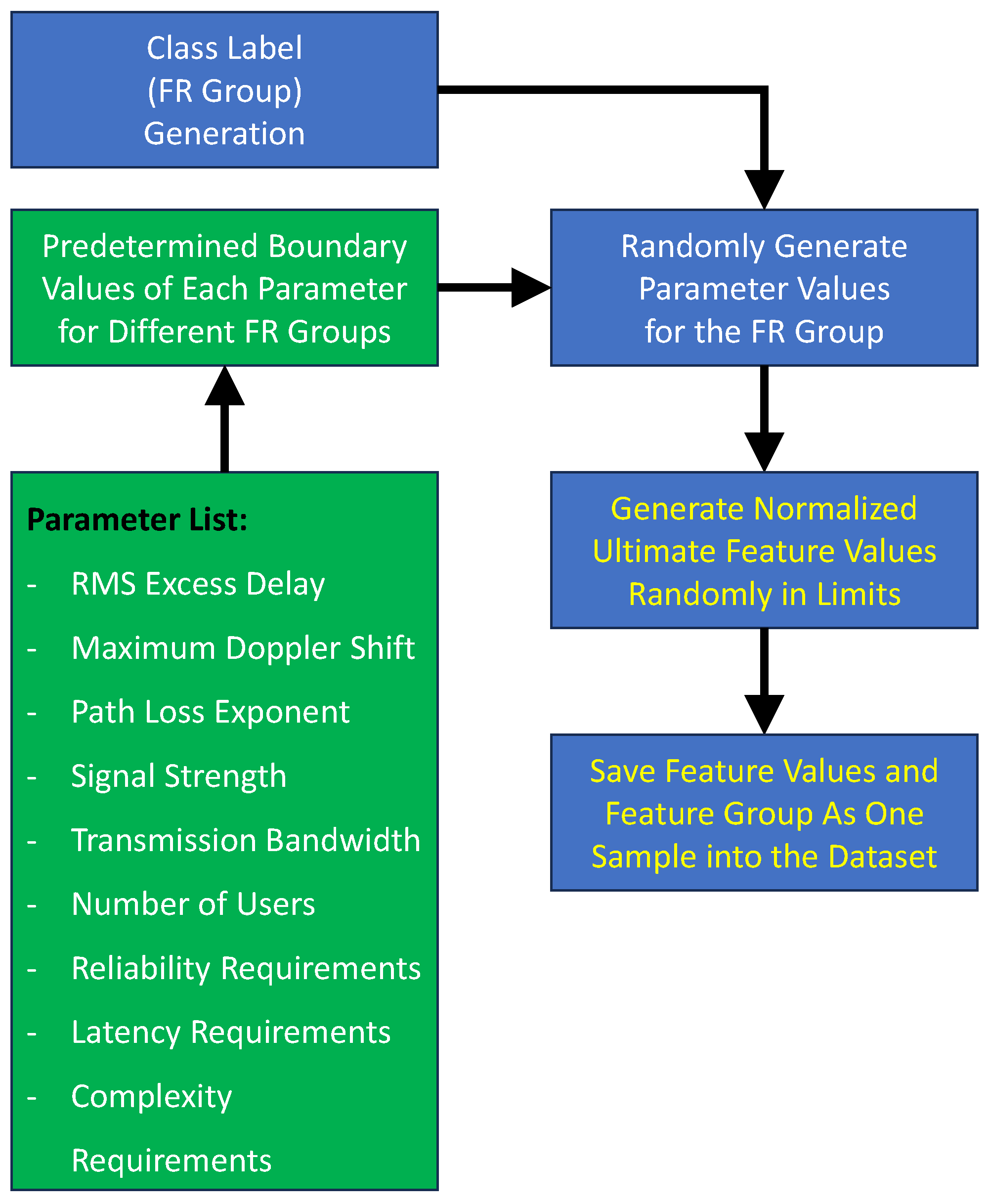
As illustrated in Figure 4, the construction of the synthetic dataset begins with the generation of FR group class labels, followed by the creation of feature values. These features are produced with an element of randomness, guided by the assigned FR groups and their corresponding wireless channel characteristics. Prior to this process, upper and lower bounds are defined to frame the variability of scenario parameters. The entire dataset generation is implemented through a MATLAB script. It is assumed that the resulting feature values are scaled to fall within a normalized range of 1 to 10. Accordingly, basic/rural/scarce/indoor scenarios are mapped to a value of 1, whereas extreme/urban/dense/outdoor scenarios correspond to a value of 10 in the dataset. For instance, if the scenario reflects a harsh environment, the normalized value of the geographic characteristic feature is assigned as 10.

Table 4. Feature definitions for the generated dataset. GIS: Geographic information system; TP: Transmission point; eMBB: Enhanced mobile broadband; URLCC: Ultra-reliable low-latency communications; mMTC: Massive machine-type communications; Info. Gain: Information Gain.

No	Definition	Source	Relations	Range	Info. Gain
1	Geographic Characteristic	GIS	Harsh environments give rise to complex multipath effects. mmWave frequencies may not be suitable for extreme environments.	Basic (1) – Extreme (10)	0.208
2	Residential Area Plan	GIS	Urban scenarios are highly susceptible to rich multipath propagation. Path loss characteristics vary significantly considering this feature. mmWave frequencies may not be suitable for rural scenarios.	Rural (1) – Urban (10)	0.033
3	General Weather Conditions	GIS	Path loss characteristics exhibit notable variation. There is a high likelihood of increased interference. mmWave frequencies may not be suitable for extreme weather conditions.	Basic (1) – Extreme (10)	0.033
4	Vehicle Traffic Density	GIS	High mobility can introduce Doppler spread. Close connection with the URLLC services. Fulfilling URLLC requirements necessitates both low delay spread and low Doppler spread. mmWave frequencies may not be suitable for dense vehicle traffic conditions.	Scarce (1) – Dense (10)	0.355
5	User Density	TP	Spectral efficiency is a critical criterion. Closely associated with the eMBB services. Requires increased channel capacity. mmWave frequencies may be more suitable for ultra-dense user scenarios.	Scarce (1) – Dense (10)	0.210
6	Indoor Outdoor Usage	TP	Path loss characteristics exhibit notable variation. There is a high likelihood of increased interference. mmWave frequencies may not be suitable for indoor usage conditions with the outdoor TP.	Indoor (1) – Outdoor (10)	0.355
7	IoT System Density	TP	Close connection with the mMTC services. Path loss characteristics play a key role in meeting mMTC requirements. mmWave frequencies may not be suitable for long-range IoT communication scenarios.	Scarce (1) – Dense (10)	0.333

outlines the representative associations between scenario parameters and wireless communication channel characteristics. Among these, geographic structure and the layout of residential areas exhibit a strong correlation with the degree of multipath propagation observed in the channel. Additionally, several features—including residential area configuration, prevailing weather conditions, indoor versus outdoor environments, and the density of IoT systems—play a significant role in shaping the path loss behavior of the wireless link. For the vehicle traffic density feature, especially Doppler spread effects are important while forming a relationship with the FR groups. The other feature, user density, affects the decision for the amount of BW usage considering the FRs. Transmission BW affects the frequency selectivity. Additionally, vehicle traffic density, user density, and IoT system density features have relations with the user requirements. The generation of synthetic data is justified by the need to explore parameter ranges not fully available in measurement campaigns. For example, antenna heights are varied between 3 and 15 m and inter-site distances between 50 and 200 m to cover realistic urban microcell and macrocell scenarios. The dataset generation pipeline is simplified into three steps: (1) environment parameter sampling, (2) channel response simulation, and (3) feature extraction for ML models. Selected features are adequate because they directly influence mmWave propagation. Constraints of synthetic data include limited capture of hardware imperfections and rare blockage events.

4. Results and Discussion

In this section, a synthetic dataset is first generated based on the wireless channel relationships described in the previous section. Next, the results of several supervised ML algorithms applied to the generated synthetic dataset are presented. Then, different scenarios are explored, and the comparison outcomes are presented to underscore the effectiveness of the proposed methodology. Finally, research limitations are discussed with different aspects.

4.1. Machine Learning Results

The ML experiments are implemented using Python 3.10, scikit-learn (v1.3), and Orange Data Mining (v3.39). Dataset generation is performed in MATLAB R2023b on a Windows desktop environment. For the hardware, Intel Core i7 processor and 32 GB RAM are employed during the simulations and ML experiments.

For evaluating the performance of the ML models, a synthetic dataset with 10,000 samples and uniformly distributed class labels is created. The dataset is split into training (70%), validation (15%), and test (15%) subsets with stratification across FR groups. In addition, 5-fold cross-validation is conducted to confirm the robustness of results. The experiments in supervised learning are performed using the Orange Data Mining software and the scikit-learn Python library [35]. A comparative analysis is performed among several algorithms, including neural networks (NNs), gradient boosting (GB), k-nearest neighbors (kNN), and random forest (RF). Each model undergoes hyperparameter optimization to ensure fair evaluation [36]. Performance metrics, namely, classification accuracy and F1 score, are calculated based on the formulations given in Equations (5)–(8). The optimized hyperparameters and corresponding performance outcomes are summarized in

Table 5. The best hyperparameters and corresponding ML results.

Model	Optimized Hyperparameters	Accuracy	F1 Score
Neural Networks (NNs)	Activation: ReLu Solver: Adam Alpha: 0 Hidden Layers: 10 Number of iterations: 500	0.795	0.0.794
Gradient Boosting (GB)	Learning rate: 0.1 Max depth: 3 Min sample split: 2 Number of estimators: 200	0.790	0.790
k-Nearest Neighbors (kNN)	Metric: Euclidean Number of neighbors: 20	0.779	0.779
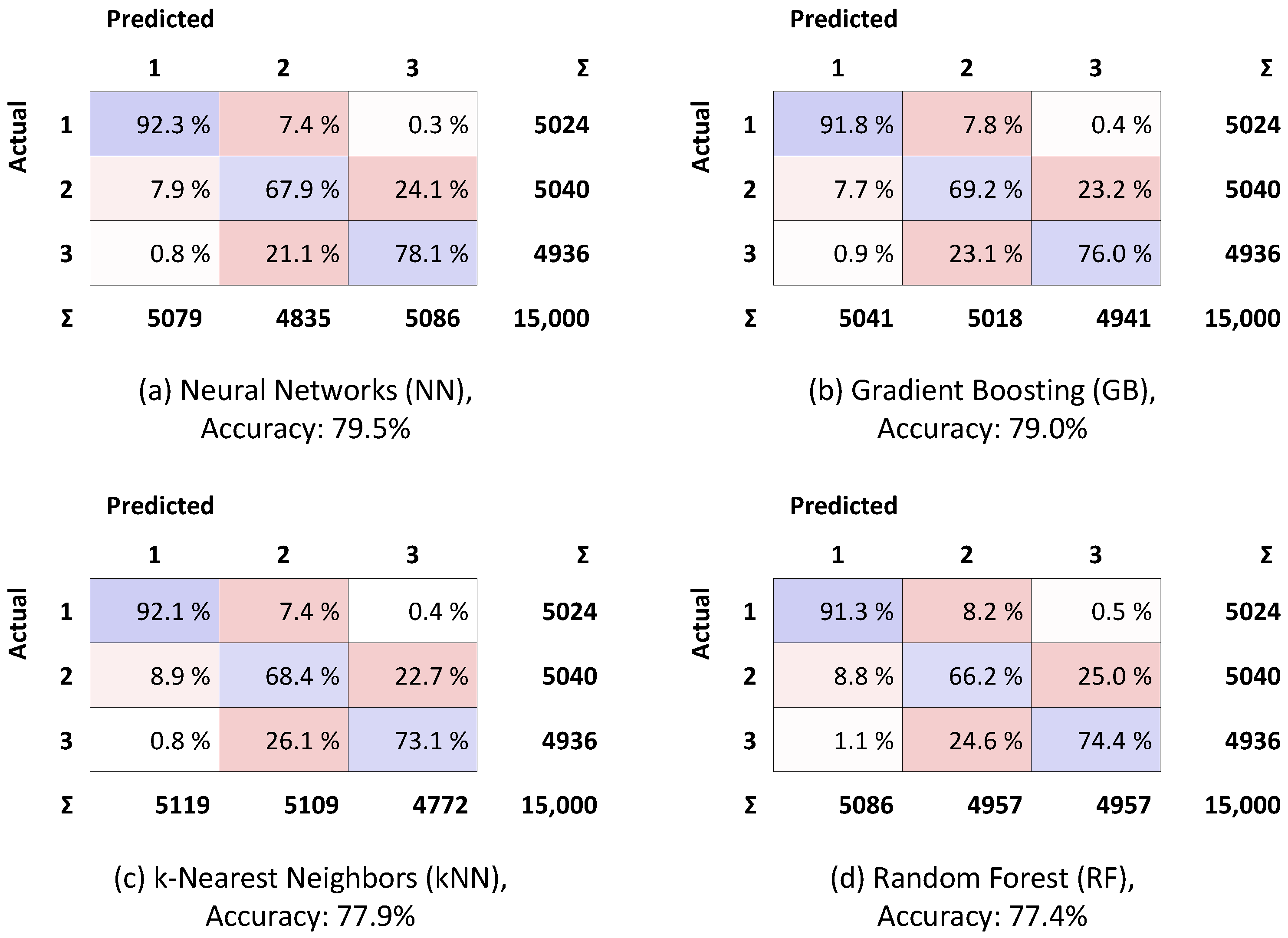
Random Forest (RF)	Min sample split: 5 Number of estimators: 20	0.774	0.774

, while the confusion matrices for each model are illustrated in Figure 5. Moreover, feature importance analysis is performed using information gain metric. The results are presented in the last column of Table 4 to show which features are most critical for the decisions.

$$\begin{array}{c}\hfill Accuracy={\displaystyle \frac{TP+TN}{TP+FN+TN+FP}}\end{array}$$

(5)

$$\begin{array}{c}\hfill Precision={\displaystyle \frac{TP}{TP+FP}}\end{array}$$

(6)

$$\begin{array}{c}\hfill Recall={\displaystyle \frac{TP}{TP+FN}}\end{array}$$

(7)

$$\begin{array}{c}\hfill F1Score={\displaystyle \frac{2\times Precision\times Recall}{Precision\times Recall}}\end{array}$$

(8)

where the abbreviations TP, FN, TN, and FP mean true positive, false negative, true negative, and false positive, respectively.

In the NN model, a single hidden layer comprising 10 neurons is employed, with the maximum iteration count configured as 500. This setup yields a classification accuracy of 79.5% and an F1 score of 0.794. For the GB algorithm, the model is configured with a maximum tree depth of 3, a total of two trees, and a learning rate of 0.1. Under this configuration, the GB model attains a classification accuracy of 79.0% alongside an F1 score of 0.790. In the case of the kNN model, the Euclidean distance metric is selected, and the number of neighbors is set to 20. This results in a classification accuracy of 77.9% and an F1 score of 0.779. The RF model, utilizing 20 estimators, achieves a classification accuracy of 77.4% with a corresponding F1 score of 0.774. Given the balanced nature of the dataset, the performance differences between accuracy and F1 score across the models remain minimal. Beyond accuracy and F1, per-class precision and recall (sensitivity) results are also presented for the employed ML models in

Table 6. Per-class performance metrics for the NN model.

FR Group	Precision	Recall	F1 Score
FR1	0.892	0.923	0.907
FR2-1	0.729	0.679	0.703
FR2-2	0.758	0.781	0.769

,

Table 7. Per-class performance metrics for the GB model.

FR Group	Precision	Recall	F1 Score
FR1	0.891	0.918	0.904
FR2-1	0.719	0.692	0.705
FR2-2	0.740	0.760	0.750

,

Table 8. Per-class performance metrics for the kNN model.

FR Group	Precision	Recall	F1 Score
FR1	0.894	0.921	0.907
FR2-1	0.703	0.684	0.693
FR2-2	0.740	0.731	0.735

and

Table 9. Per-class performance metrics for the RF model.

FR Group	Precision	Recall	F1 Score
FR1	0.890	0.913	0.901
FR2-1	0.686	0.662	0.674
FR2-2	0.728	0.744	0.736

.

Among the evaluated models, the NN algorithm delivers the highest accuracy for Class-1 (FR1), reaching 92.3%. For Class-2 (FR2-1), the GB model stands out with the best performance, achieving an accuracy of 69.2%. Regarding Class-3 (FR2-2), the NN model again shows strong performance, obtaining an accuracy of 78.1%. Upon examining the results, it is observed that the success rates range between 77% and 80%. Notably, the NN model stands out, delivering slightly better results than the other algorithms. The GB algorithm provides performance nearly on par with the NN model. As a main difference NN performed better in complex feature interactions due to nonlinear modeling, while GB showed strength in handling imbalanced sub-patterns. These findings suggest implications for selecting lightweight vs. more complex ML models depending on deployment needs.

4.2. Comparison Results

The results for different scenario definitions are given in

Table 10. Comparison results under different scenario definitions.

No	Scenario Definition	FR1		FR1, FR2-1, and FR2-2
		General User Satisfaction	Additional TP Investment	General User Satisfaction	Additional TP Investment
1	Single-family houses in a simple environment (e.g., lowland)	Medium	Not Necessary	High	Necessary
2	Single-family houses in a harsh environment (e.g., forestland)	High	Not Necessary	High	Not Necessary
3	Dispersed settlement in a mountainous terrain	High	Not Necessary	High	Not Necessary
4	Residential area in a suburban area	Low	Not Necessary	High	Necessary
5	City center with tower blocks	High	Not Necessary	High	Not Necessary
6	City center with low-rise buildings and low vehicle traffic under an arid climate	Low	Not Necessary	High	Necessary
7	City center in the rainy region	High	Not Necessary	High	Not Necessary
8	City center with dense vehicle traffic	High	Not Necessary	High	Not Necessary
9	Urban scenario with a high population	Medium	Not Necessary	High	Necessary
10	Crowded city center in a metropolis	Low	Not Necessary	High	Necessary
11	Smart city region with broad IoT usage	High	Not Necessary	High	Not Necessary

. The NN algorithm is used for the scenario-based comparison results. The following 11 scenarios are analyzed:

1.

Single-family houses in a simple environment;

2.

Single-family houses in a harsh environment;

3.

Dispersed settlement in a mountainous terrain;

4.

Residential area in a suburban area;

5.

City center with tower blocks;

6.

City center with low-rise buildings and low vehicle traffic under an arid climate;

7.

City center in the rainy region;

8.

City center with dense vehicle traffic;

9.

Urban scenario with a high population;

10.

Crowded city center in a metropolis;

11.

Smart city region with broad IoT usage.

The Table 10 results (user satisfaction and TP investment necessity) are derived by mapping the predicted FR classes under each scenario to expected coverage and capacity levels, and then interpreted using expert knowledge of deployment trade-offs.

Two cases are compared to each other under these scenarios from the general user satisfaction and additional TP investment necessity perspectives. For the first case, the available frequency bands are taken only under FR1, similar to LTE coverage. For the second case, the available frequency bands for a whole region are taken as FR1, FR2-1, and FR2-2. Therefore, mmWave frequencies are included in the second case.

There is a trade-off between general user satisfaction and the need for additional TP investments. When the available frequency bands cover the 5G mmWave radio spectrum, general user satisfaction is high in all scenarios. However, additional TP investments are required in some scenarios (1, 4, 6, 9, and 10) to ensure complete coverage of the entire region.

Restating what the two cases (“Case A: FR1 only”’ vs. “Case B: FR1 + FR2-1 + FR2-2”’) represent helps make the causes of the observed differences explicit. Case A corresponds to using sub-6 GHz bands exclusively; this yields larger per-site coverage, better penetration, and more robust links under blockage or adverse weather, but limited instantaneous bandwidth per user. Case B includes mmWave bands. These provide very large bandwidths and high peak throughput but suffer from higher path loss, poor penetration, and greater sensitivity to blockage and mobility. The trade-offs that we observe in Table 10 directly follow from these physical and service characteristics.

(1) Densification planning: Adoption of mmWave (Case B) typically requires densification to achieve the same coverage probability as FR1. Planners should therefore translate model FR-class outputs into an explicit required TP density estimate (e.g., using path-loss and link-budget models or ray-tracing) before committing capital expenditures.

(2) Hybrid deployments and multi-connectivity: The practical deployment strategy suggested by the results is hybrid: maintain FR1 layers for blanket coverage and reliability, and deploy FR2 cells selectively in high-demand micro/metro hotspots. The model’s per-TP recommendation should be paired with a rule that enforces FR1 fallback (multi-connectivity) for user sessions when mmWave links fail.

(3) Cost–benefit framing: Improved user satisfaction under Case B must be weighed against CAPEX and OPEX increases (site leasing, backhaul capacity, power, and maintenance). For each region, planners should compute a simple cost model (additional TPs × site cost + enhanced backhaul) versus estimated revenue or QoE gain to decide whether the mmWave rollout is justified.

(4) Backhaul and edge compute dimensions: mmWave TPs often demand higher fronthaul/backhaul capacity and more edge compute for real-time beamforming and local ML inference. These infrastructure implications must be included in the regional aggregation stage of the planner.

In summary, the performance differences in Table 10 arise naturally from the physical trade-offs between coverage (FR1) and capacity (FR2). Translating model outputs into deployment decisions requires (i) converting FR-class recommendations to TP density and backhaul requirements via propagation/coverage models, (ii) applying confidence gating to avoid costly misdeployments, and (iii) conducting cost–benefit and sensitivity analyses so operators can select where and when mmWave densification is economically justified.

4.3. Research Limitations

This study relies on a synthetic dataset due to the lack of publicly available real-world data. While synthetic datasets enable balanced and flexible experiments, they may not fully capture complex propagation phenomena. Future validation with real-world measurement campaigns, channel sounding, or ray-tracing tools (e.g., WinProp and Remcom) is necessary. Another limitation is the assumption of idealized feature distributions; sensitivity analyses mitigate this partially, but generalization challenges remain. Domain adaptation and transfer learning are proposed for future work.

5. Conclusions

In this paper, a new concept is developed for the smart spectrum recommendation approach with edge learning for 5G and beyond radio planning. Incorrect selection of FR can be prevented when radio planning is conducted from the spectrum perspective. It is observed that benefits can be obtained in utilizing mmWave frequencies through the ML-based method by producing data-driven recommendation decisions. Thus, the entire region can be analyzed for full coverage during the 5G transition using this study. Environment awareness and the use of ambient intelligence are two strong aspects of the proposed approach.

In the future, the availability of a real-world dataset for the same problem definition may introduce a generalization challenge when applying ML models trained on synthetic data. To address the potential domain adaptation problem, preprocessing techniques and transfer learning methods can be employed. Furthermore, future studies may consider increasing the number of input values and feature definitions to enhance model performance and representational capacity. Thereafter, feature selection and dimensionality reduction techniques may be applied to the dataset. For the ML approaches, different types of cascading models can be tested. Moreover, more specific frequency bands can be recommended as the output. Additionally, the locations of new TPs can be efficiently determined by recursively applying the proposed approach.

Beyond these findings, several prospects for further research are noteworthy. First, the proposed framework can be extended to support 6G networks, where even higher frequency ranges (sub-THz) and new service types such as holographic communications and massive digital twins will impose stricter requirements on spectrum planning. Second, the operational cost implications of distributed edge learning must be analyzed in detail. While edge-based decision making reduces backhaul and central processing demands, it introduces costs in terms of computational resources at each transmission point; therefore, a cost–benefit analysis for operators is essential. Finally, future work should address compliance with evolving 3GPP standards, as spectrum allocation, carrier aggregation, and AI-native network functionalities continue to evolve. Aligning the proposed framework with these standards will ensure practical applicability and industry adoption.