Enhancing the Sustained Capability of Continual Test-Time Adaptation with Dual Constraints

Abstract

Continuous Test-Time Adaptation aims to adapt a source model to continuously and dynamically changing target domains. However, previous studies focus on adapting to each target domain independently, treating them as isolated, while ignoring the interplay of interference and promotion between domains, which limits the model’s sustained capability, often causing it to become trapped in local optima. This study highlights this critical issue and identifies two key factors that limit the model’s sustained capability: (1) The update of parameters lacks constraints, where domain-sensitive parameters capture domain-specific knowledge, leading to unstable channel representations and interference from old domain knowledge and hindering the learning of domain-invariant knowledge. (2) The decision boundary lacks constraints, and distribution shifts, which carry significant domain-specific knowledge, cause features to become dispersed and prone to clustering near the decision boundary. This is particularly problematic during the early stages of domain shifts, where features are more likely to cross the boundary. To tackle the two challenges, we propose a Dual Constraints method: First, we constrain updates to domain-sensitive parameters by minimizing the representation changes in domain-sensitive channels, alleviating the interference among domain-specific knowledge and promoting the learning of domain-invariant knowledge. Second, we introduce a constrained virtual decision boundary, which forces features to move away from the original boundary, and with a virtual margin to prevent features from crossing the decision boundary due to domain-specific knowledge interference caused by domain shifts. Extensive benchmark experiments show our framework outperforms competing methods.

1. Introduction

Continual Test-Time Adaptation (CTTA) focuses on enhancing machine learning models’ ability to adapt continuously in dynamic environments where input data distributions shift over time. This capability is crucial in various real-world scenarios. For instance, in autonomous driving [1,2,3,4], a vehicle may encounter changing conditions such as transitioning from daylight to nighttime or from sunny to rainy weather. To maintain high performance, models must adapt effectively to these evolving data distributions through Continual Test-Time Adaptation.

Numerous methods have been developed to tackle the challenges of Continual Test-Time Adaptation, including the use of teacher–student models [5,6,7], data augmentation techniques [5], semi-supervised learning [8], Low-Rank Learning [9], sample replay [10], and Masked Autoencoders [11].

Although previous studies have achieved significant success, a key limitation must be pointed out: These studies still follow the approach of Test-Time Adaptation (TTA) [12], treating the problem of Continual Test-Time Adaptation in isolation and focusing solely on adapting to each domain independently. This limits the model’s sustained capability, similar to a greedy algorithm [13], causing the model’s performance to become trapped in local optima [14] and failing to achieve the ideal global optimum [15]. This is because these methods overlook the essential nature of Continual Test-Time Adaptation: in this setting, domain adaptation is dynamic, ongoing, and continuously evolving, resulting in different domains either interfering with or promoting each other.

Therefore, addressing the following two challenges is crucial for enhancing the sustained capability of Continual Test-Time Adaptation: (1) How to effectively alleviate the mutual interference of domain-specific knowledge. (2) How to effectively learn domain-invariant knowledge across domains.

This study revisits the differences between Continual Test-Time Adaptation and Test-Time Adaptation, focusing on the long-neglected issue of sustained capability, and identifies two key factors that severely limit the model’s sustained capability and prevent it from getting trapped in local optima:

• Lack of constraints in parameter updates: The model contains a large number of domain-sensitive parameters, which tend to learn domain-specific knowledge. When the model encounters a new domain, the distribution difference between the old and new domains causes these domain-sensitive parameters to behave abnormally, leading to unstable channel representations that incorporate substantial domain-specific knowledge from previous domains, especially in the early stages of adapting to the new domain. This results in severe interference between domain-specific knowledge. More importantly, relying on domain-specific knowledge for classification significantly hinders the learning of domain-invariant knowledge.
• Lack of constraints in decision boundary: Domain shifts carry a significant amount of domain-specific knowledge, causing the features generated by the model to spread out more. The lack of constraints makes these features prone to clustering near or crossing the decision boundary. Under the interference of domain-specific knowledge, features near the decision boundary are more likely to cross, particularly in the early stages of the new domain.

As shown in Figure 1, we analyze the channel representations under three different corruption levels (level-5, level-3, and level-1) of CIFAR10C (The method for calculating unstable channel representations is provided in Section 4.4.3). In Figure 1a, we observe that different levels of corruption have varying impacts on the stability of channel representations. The higher the level of corruption, the more unstable the channel representations become. The domain-sensitive parameters are highly sensitive to this domain-specific knowledge, resulting in anomalies and instability in the channel representations.

In Figure 1b, we observe that domain-sensitive channels are much more responsive to domain shifts than domain-robust channels. When encountering different domains, the representation of these channels tends to exhibit instability and are prone to significant variations. The cause of this abnormal behavior lies in the domain-sensitive parameters, which tend to overfit domain-specific knowledge such as background, lighting, and texture. When a domain shift occurs, this domain-specific knowledge undergoes drastic changes, leading to significant variations in the channel representations. The instability of channel representations and the presence of a large amount of domain-specific knowledge can cause significant interference in domain adaptation, especially in the early stages of domain shift. In contrast, domain-robust parameters focus on learning domain-invariant knowledge, such as contours and shapes. This domain-invariant knowledge remains unaffected by domain shifts, resulting in more stable channel representations.

Based on our observation in Figure 1, we can see that domain-specific channels exhibit instability and are prone to change. Therefore, we propose a parameter update constraint method that estimates the relationship between changes in channel representations and the loss increases caused by parameter updates, suppressing domain-sensitive parameters by minimizing the changes in domain-sensitive channel representations. This constraint not only effectively alleviates the interference caused by domain-specific knowledge but also promotes the learning of domain-invariant knowledge by reducing the sensitivity of the parameters. Additionally, we provide theoretical evidence that our method can effectively enhance the model’s generalization ability and promote the learning of domain- invariant knowledge.

Furthermore, as shown in Figure 2, domain shifts carry substantial domain-specific knowledge, and when the model has not yet adapted to the new domain, features are more susceptible to the effects of the domain shift, making them more likely to cross the original decision boundary. We introduce a virtual decision boundary that constrains the features generated by the model to move away from the original decision boundary, preventing them from clustering near it. This constraint also creates a virtual margin between two decision boundaries. During domain shifts, this virtual margin provides sufficient buffering to prevent features from crossing the original decision boundary. The strongly constrained virtual decision boundary effectively mitigates the interference caused by domain-specific knowledge in the early stages of domain adaptation.

Overall, we propose a Dual Constraints method that combines channel-based parameter constraints and feature-based virtual decision boundary constraints, effectively addressing the two major challenges of domain knowledge interference and learning domain-invariant knowledge, thereby enhancing the model’s sustained capability(More motivations and details will be elaborated in Section 3.1). Our contributions can be summarized as follows:

• We propose a novel parameter constraint method that minimizes the representation changes in domain-sensitive channels, which, respectively, enhance and suppress the learning of domain-invariant and domain-specific knowledge. In addition, we theoretically prove that it can effectively enhance the model’s generalization ability.
• We introduce a strongly constrained virtual decision boundary that creates a virtual margin, forcing features away from the original decision boundary, effectively mitigating the problem of features crossing the boundary during domain shifts.
• Dual Constraints enhance the model’s sustained capability and achieve excellent performance, surpassing all existing state-of-the-art methods.

2. Related Work

2.1. Unsupervised Domain Adaptation

Unsupervised Domain Adaptation (UDA) [16] assumes that there is a domain shift between the source domain and the target domain, with labeled data available in the source domain but no labels in the target domain [17]. The goal is for the model to perform well on the unlabeled target domain data. UDA methods often use distribution distance metrics to align the feature distributions between the source and target domains during training. For example, Maximum Mean Discrepancy (MMD) [18,19,20] is a statistical test that assesses whether two distributions are equal based on observed samples from those distributions. Adversarial training [21,22,23] is another common approach, which involves aligning distributions using two adversarial roles: a domain classifier and a feature generator. Unlike traditional Unsupervised Domain Adaptation methods, Test-Time Adaptation (TTA) aims to adapt a model trained on a source domain to a new target domain without accessing the original source data during inference, and many methods have been proposed to solve TTA, such as TENT [12] and SHOT [24]. TENT [12] updates the trainable batch normalization parameters from a pretrained model by minimizing the entropy of the model’s predictions during testing. SHOT [24] combines entropy minimization and diversity regularization with label smoothing techniques to train a general feature extractor from the pretrained source model.

2.2. Domain Generalization

Domain generalization (DG) aims to extract knowledge from the source domain that can generalize well to unseen target domains. Many methods learn domain-invariant representations by aligning the distributions of the target and source domains. These methods include adversarial learning [25], causal learning [26], and meta-learning [27]. Another approach is to enhance the model’s generalization capability by generating more source domain data, specifically by augmenting the diversity of the source data through data augmentation [28]. These data augmentation techniques primarily involve style transfer [28,29] and pixel-level augmentation [30]. Although these methods have demonstrated promising results, they may still learn excessive domain-specific features, as they rely on implicit assumptions to remove domain-specific characteristics via image-level augmentation or model-level constraints. Some studies have pointed out that Convolutional Neural Networks (CNNs) tend to classify objects based on local texture features that contain domain-specific characteristics [31,32,33]. To address this, they propose using penalty loss functions to suppress the model from learning local features such as texture, background, and lighting. This penalty encourages the model to rely on global features for classification. In contrast to local features, global features, including shape and contours, remain more stable and less prone to changes across domains. Therefore, this penalty on local features forces the model to learn domain-invariant properties, thereby enhancing its generalization ability.

2.3. Continual Learning

Continual learning (CL) aims to enable models to learn new tasks from a continuously evolving data stream while retaining previously acquired knowledge. One of the main challenges is catastrophic forgetting, where models tend to forget prior knowledge when learning new tasks. To address this issue, several approaches have been proposed, including regularization methods [34], which protect important weights from excessive updates, architecture expansion methods [35], which adapt the model by expanding its structure to accommodate new tasks, and memory replay methods [36,37,38,39], which store and replay data from previous tasks to mitigate forgetting. Despite significant progress, continual learning still faces challenges related to computational and memory overhead and maintaining strong generalization performance under non-stationary data distributions.

2.4. Continual Test-Time Adaptation

Unlike traditional Test-Time Adaptation (TTA) [40,41,42], which assumes a fixed target domain and works in a source-free online manner, CTTA accounts for the dynamic nature of real-world data distributions. This means CTTA requires models to adapt online and source-free across evolving domains. CoTTA [5] is a leading approach in continual domain learning, using average teachers and data augmentation for reliable pseudo-labels and robust model updates. DSS [8], inspired by semi-supervised learning, employs FreeMatch [43] to generate label thresholds for filtering pseudo-labels. RoTTA [44] stabilizes Batch Normalization updates to mitigate batch size variations during adaptation. RMT [6] addresses asymmetry in cross-entropy in teacher–student models, proposing symmetric cross-entropy for better gradients. Reshaping [10] addresses the catastrophic forgetting problem using sample replay. MAE [11] leverages mask autoencoders to learn domain-invariant knowledge. Unlike previous work, this study focuses on the sustainability of continuous domain adaptation, aiming to find the global optimum rather than settling for local optima.

3. Method

3.1. Problem Setting

Given a pretrained model $M^0$ with initial parameters ${\theta }_0$, originally trained on source domain data $(X^S,Y^S)$, the objective of CTTA is to iteratively adapt model M to a sequence of target domain datasets. During this process, the source domain data $(X^S,Y^S)$ is not accessible, and the target domain datasets $\{X_0^T,X_1^T,\dots ,X_n^T\}$ are unlabeled. At each time step t, the parameters ${\theta }_t$ are updated to ${\theta }_{t+1}$ to better align the model $M^{t+1}$ with the current target domain $X_t^T$. For the sake of clarity, we define the model output as: $\widehat{y}=M\left(x\right)=G\left(Z\right)=G_{\ell }\left(F_{\ell }\left(x\right)\right)$. $F\left(x\right)$ is the feature extractor, and the feature map at the ${\ell }^{th}$ layer is $Z_{\ell }=\{Z_{\ell ,1},Z_{\ell ,2},\dots ,Z_{\ell ,C_{\ell }}\}=F_{\ell -1}\left(Z_{\ell -1}\right)$, where $Z_{\ell }\in {\mathbb{R}}^{C_{\ell }\times H_{\ell }\times W_{\ell }}$. $G(·)$ represents the classifier, and $W=\{W_1,W_2\dots W_C\}$ denotes the weights of the classifier.

3.2. Domain-Sensitive Parameter Suppression

3.2.1. Motivation of Domain-Sensitive Parameter Suppression

Existing methods typically use the following objective function to optimize model parameters for domain adaptation during testing:

$$\underset{M^{t+1}}{min}\mathcal{L}(M^{t+1}\left(X_t^T\right),{\widehat{Y}}_t^T)$$

(1)

where at time t, the target domain data $X_t^T$ is encountered, and the model parameters are updated based on the loss function $\mathcal{L}(·)$ to form the new model $M^{t+1}$. It is important to note that before any parameter update at time t, $M^{t+1}=M^t$.

Existing methods naively use Equation (1) as the objective function, leading to an unconstrained parameter update process. A large amount of domain-sensitive parameters are highly sensitive to domain-specific knowledge and change rapidly to fit such knowledge [31,45], such as background, lighting, and texture. Although existing methods introduce EMA [46], where $M^t=\beta M^{t-1}+(1-\beta )M^t$, and set $\beta =0.999$ to alleviate performance degradation caused by rapid parameter changes, this parameter weighting approach has several issues: historical parameters contain a large amount of knowledge from past domains, which interferes with the current domain adaptation process, and hyperparameters cannot be adjusted adaptively. Moreover, this method is often used as a performance-boosting technique: people know that using it improves performance, but not using it worsens performance, without exploring the essence of the problem.

3.2.2. Implementation of Domain-Sensitive Parameter Suppression

To tackle this challenge, we propose a novel parameter constraint method that minimizes the representation changes in domain-sensitive channels, effectively mitigating the rapid updates and overfitting of domain-sensitive parameters to domain-specific knowledge.

Now, we consider two consecutive models, $M^t$ and $M^{t-1}$. Theoretically, the parameter difference between two adjacent models is very small, but CTTA is a continuous process where the model continuously adapts to the target domain, which will eventually result in a huge cumulative effect. To analyze the feature maps change caused by the model parameter changes between adjacent moments, let $Z_{\ell }^{\prime }$ and $Z_{\ell }$ are the feature maps generated by the $\ell -1^{th}$ layer of $M^t(·)$ and $M^{t-1}(·)$, respectively. We can compute the loss given by $Z_{\ell }^{\prime }$ via the first-order Taylor approximation as follows:

$$\begin{array}{cc}\hfill \mathcal{L}(G_{\ell }\left(Z_{\ell }^{\prime }\right),\widehat{y})& \approx \mathcal{L}(G_{\ell }\left(Z_{\ell }\right),\widehat{y})\hfill \\ \hfill & +\sum _{c=1}^{C_{\ell }}{〈{\nabla }_{Z_{\ell ,c}}\mathcal{L}(G_{\ell }\left(Z_{\ell }\right),\widehat{y}),Z_{\ell ,c}^{\prime }-Z_{\ell ,c}〉}_F\hfill \end{array}$$

(2)

where ${\langle ·,·\rangle }_F$ is the Frobenius inner product, i.e., ${\langle A,B\rangle }_F=\mathrm{tr}\left(A^{\top }B\right)$, and ${\nabla }_{Z_{\ell ,c}}\mathcal{L}(G_{\ell }\left(Z_{\ell }\right),\widehat{y})$ is the gradient in the backpropagation of $M^{t-1}(·)$. Using Equation (2), we define the loss increment $▵\mathcal{L}\left(Z_{\ell ,c}^{\prime }\right)$ for the $c^{th}$ channel at the ${\ell }^{th}$ layer caused by parameter changes as follows:

$$▵\mathcal{L}\left(Z_{\ell ,c}^{\prime }\right):={〈{\nabla }_{Z_{\ell ,c}}\mathcal{L}(G_{\ell }\left(Z_{\ell }\right),\widehat{y}),Z_{\ell ,c}^{\prime }-Z_{\ell ,c}〉}_F$$

(3)

Thus, we aim to minimize the loss change caused by parameter updates between two adjacent models at consecutive moments, as follows:

$$\underset{M^{t+1}}{min}\sum _{\ell =1}^L\sum _{c=1}^{C_{\ell }}{\mathbb{E}}_{\left(x\right)\sim X_t^T}{\left[▵\mathcal{L}\left(Z_{\ell ,c}^{\prime }\right)\right]}^2$$

(4)

We need to update $M_t(·)$ to $M_{t+1}(·)$ at time t using data $X_t^T$. If we minimize Equation (4) using standard stochastic gradient descent, in addition to calculating the gradients of the feature maps produced by $M^t(·)$ with respect to the samples, we also need to calculate and store the gradients of the feature maps produced by $M^{t-1}(·)$ with respect to the samples, which significantly increases computational cost or memory overhead.

Using the Cauchy-Schwarz inequality, we derive the upper bound for the objective function of Equation (4) as follows:

$$\mathbb{E}\left[▵\mathcal{L}\left(Z_{\ell ,c}^{\prime }\right)\right]$$

$$=\mathbb{E}\left[{\langle {\nabla }_{Z_{\ell ,c}}\mathcal{L}(G_{\ell }\left(Z_{\ell }\right),\widehat{y}),Z_{\ell ,c}^{\prime }-Z_{\ell ,c}\rangle }_F\right]$$

$$\le \mathbb{E}\left[\parallel {\nabla }_{Z_{\ell ,c}}\mathcal{L}(G_{\ell }\left(Z_{\ell }\right),\widehat{y}){\parallel }_F·{\parallel Z_{\ell ,c}^{\prime }-Z_{\ell ,c}\parallel }_F\right]$$

$$\le \sqrt{\mathbb{E}\left[\parallel {\nabla }_{Z_{\ell ,c}}\mathcal{L}(G_{\ell }\left(Z_{\ell }\right),\widehat{y}){\parallel }_F^2\right]·\mathbb{E}\left[\parallel Z_{\ell ,c}^{\prime }-Z_{\ell ,c}{\parallel }_F^2\right]}$$

(5)

By optimizing the upper bound of the objective function, we avoid storing large amounts of the gradients of the feature maps or performing additional backpropagation. Substituting Equation (5) into the objective function to minimize Equation (4), we obtain

$$\underset{M^{t+1}}{min}\sum _{\ell =1}^L\sum _{c=1}^{C_{\ell }}{\mathbb{E}}_{x\sim X_t^T}\parallel {\nabla }_{Z_{\ell ,c}}\mathcal{L}(G_{\ell }\left(Z_{\ell }\right),\widehat{y}){\parallel }_F^2·{\parallel Z_{\ell ,c}^{\prime }-Z_{\ell ,c}\parallel }_F^2$$

(6)

According to Figure 3, we observe an interesting phenomenon: The degree of unstable representation of the channels is positively correlated with the magnitude of the gradient values. Larger gradients cause the parameters to change rapidly, indicating that domain-sensitive parameters are sensitive to domain-specific knowledge and fit such knowledge through rapid changes, leading to unstable channel representations that are prone to variations and contain a large amount of domain-specific knowledge. This is consistent with the conclusion derived from the Equation (6): the larger the gradient value, the higher the degree of suppression of the parameters.

Therefore, we define a channel sensitivity importance weight as $I_{\ell ,c}^t$:

$$I_{\ell ,c}^t={\parallel {\nabla }_{Z_{\ell ,c}}\mathcal{L}(G_{\ell }\left(Z_{\ell }\right),\widehat{y})\parallel }_F^2$$

(7)

However, we cannot directly optimize using this equation. There are significant differences in the magnitude of channel gradients across layers, so it is necessary to balance the scale of importance across layers. Finally, we construct the channel sensitivity importance weight $I_{\ell ,c}^t$ as follows:

$$I_{\ell ,c}^t=\left\{\begin{array}{cc}{I}_{\ell ,c}^t=0\hfill & t=0\hfill \\ I_{\ell ,c}^t={\displaystyle \frac{I_{\ell ,c}^{t-1}+{\parallel {\nabla }_{Z_{\ell ,c}}\mathcal{L}(G_{\ell }\left(Z_{\ell }\right),\widehat{y})\parallel }_F^2}{\frac{1}{C_{\ell ,c}}{\sum }_{c=1}^{C_{\ell }}{\parallel {\nabla }_{Z_{\ell ,c}}\mathcal{L}(G_{\ell }\left(Z_{\ell }\right),\widehat{y})\parallel }_F^2}}\hfill & t>0\hfill \end{array}\right.$$

(8)

Therefore, the final parameter constraint objective function can be expressed as

$${\mathcal{L}}_{DSP}=\underset{M^{t+1}}{min}\sum _{\ell =1}^L\sum _{c=1}^{C_{\ell }}{\mathbb{E}}_{x\sim X_t^T}{I}_{\ell ,c}^t·{\parallel Z_{\ell ,c}^{\prime }-Z_{\ell ,c}\parallel }_F^2$$

(9)

3.2.3. Theoretical Analysis of Domain-Sensitive Parameter Suppression

In this section, we prove from the perspective of Lipschitz continuity that our method can effectively suppress domain-sensitive parameters, promote the learning of domain-invariant knowledge, and enhance the generalization ability of the model.

We first provide the definition of Lipschitz continuity. Given $\Omega \subset {\mathbb{R}}^n$, let ${\theta }_1\in \Omega$ and ${\theta }_2\in \Omega$. For a function $h:\Omega \to {\mathbb{R}}^m$, if there exists a constant K such that the following holds:

$$\parallel h\left({\theta }_1\right)-h\left({\theta }_2\right){\parallel }_2\le K{\parallel {\theta }_1-{\theta }_2\parallel }_2,\forall {\theta }_1,{\theta }_2\in \Omega$$

(10)

then, h is called Lipschitz continuous.

According to existing studies [33,47], if the loss function has a smaller Lipschitz constant K, it indicates that the loss function landscape is flatter, which consequently leads to better model generalization. On the contrary, if the Lipschitz constant K is very large, it indicates that the model parameters are highly sensitive to input variations, with even minor changes leading to drastic shifts in the model’s output, which means that the model lacks generalization ability.

Now, consider the model parameters ${\theta }_{t-1}$ and ${\theta }_t$ at two consecutive moments during continual domain adaptation. The change in the loss function can be expressed as:

$$\parallel \mathcal{L}\left({\theta }_t\right)-\mathcal{L}\left({\theta }_{t-1}\right){\parallel }_2={\parallel \mathcal{L}\left(\zeta \right)({\theta }_t-{\theta }_{t-1})\parallel }_2$$

(11)

where $\zeta =c{\theta }_t+(1-c){\theta }_{t-1}$, and $c\in [0,1]$. By applying the Cauchy-Schwarz inequality, we have

$$\parallel \mathcal{L}\left({\theta }_t\right)-\mathcal{L}\left({\theta }_{t-1}\right){\parallel }_2\le \parallel \nabla L\left(\zeta \right){\parallel }_2{\parallel {\theta }_t-{\theta }_{t-1}\parallel }_2$$

(12)

Considering ${\theta }_t={\theta }_{t-1}-\eta \nabla {\theta }_{t-1}$, we have ${\theta }_t\to {\theta }_{t-1}$, so $\nabla L\left(\zeta \right)\approx \nabla \mathcal{L}\left({\theta }_{t-1}\right)$, and the above can be rewritten as

$$\parallel \mathcal{L}\left({\theta }_t\right)-\mathcal{L}\left({\theta }_{t-1}\right){\parallel }_2\le \parallel \nabla \mathcal{L}\left({\theta }_{t-1}\right){\parallel }_2{\parallel {\theta }_t-{\theta }_{t-1}\parallel }_2$$

(13)

From Equation (13), it can be seen that minimizing $\parallel \nabla \mathcal{L}\left({\theta }_{t-1}\right){\parallel }_2$ is equivalent to minimizing the Lipschitz constant K. According to Equation (9), we have

$${\mathcal{L}}_{DSP}\propto I_{\ell ,c}^t={\parallel {\nabla }_{Z_{\ell ,c}}\mathcal{L}(G_{\ell }\left(Z_{\ell }\right),\widehat{y})\parallel }_F^2$$

(14)

Thus, based on Equation (14), penalizing the gradient norm forces the model parameters to generate smaller gradient norms, which is equivalent to reducing the Lipschitz constant of the model. As a result, the model achieves better generalization performance.

3.3. Virtual Decision Boundary

3.3.1. Motivation of Virtual Decision Boundary

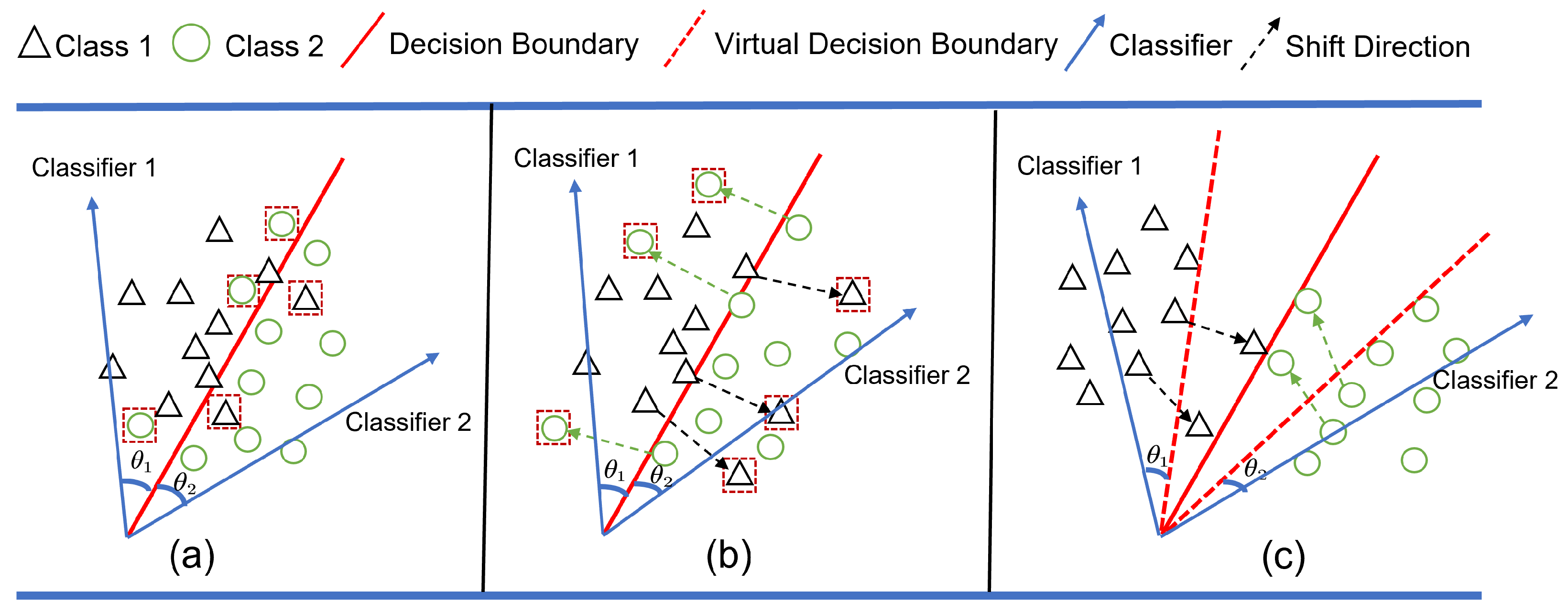
In Figure 4, we clarify the reasons behind the lack of robustness in the decision boundary and present our proposed solutions. In Figure 4a, we observe that during domain adaptation, the features extracted by the feature extractor $F(·)$ tend to cluster near or slightly cross the decision boundary, which is indicated by the red boxes. In Figure 4b, we examine domain shifts, where we assume that two successive adapted domains have deviations ${\epsilon }_k$ and ${\epsilon }_{k+1}$ from the source domain. The deviation between them is $\Delta \epsilon ={\epsilon }_{k+1}-{\epsilon }_k$. When $\Delta \epsilon >0$, the feature bias increases, leading to the possibility that features clustered near the decision boundary may cross over, resulting in errors. To address these challenges, we propose the virtual decision boundary. As shown in Figure 4c, this method introduces a virtual margin between the original decision boundary and a newly created virtual decision boundary. This virtual margin pushes features away from the original boundary, reducing the likelihood of clustering near it. Additionally, the virtual margin provides sufficient buffer space to help prevent features from crossing the decision boundary during domain shifts.

3.3.2. Implementation of Virtual Decision Boundary

Before addressing this issue, we start with a simple binary classification problem. Consider a binary classification problem where we have a sample from class 1 and use the feature extractor function $Z=F\left(x\right)$ to obtain the features of the sample x. We introduce a parameter m that is used to scale the inequality, forming a stricter virtual decision boundary. This can be mathematically expressed as $\parallel W_1{\parallel }_2{\parallel Z\parallel }_{2}cos\left(m{\theta }_1\right)>\parallel W_2{\parallel }_2{\parallel Z\parallel }_{2}cos\left({\theta }_2\right)(0\le {\theta }_1\le {\displaystyle \frac{\pi }{m}})$, where $\theta$ is the angle between the classifier vector and the feature vector, and $m\in [1,+\infty )$, as the following inequality holds:

$$\parallel W_1{\parallel }_2{\parallel Z\parallel }_{2}cos\left({\theta }_1\right)\ge \parallel W_1{\parallel }_2{\parallel Z\parallel }_{2}cos\left(m{\theta }_1\right)>\parallel W_2{\parallel }_2{\parallel Z\parallel }_{2}cos\left({\theta }_2\right)$$

(15)

Therefore, $\parallel W_1{\parallel }_2{\parallel Z\parallel }_{2}cos\left({\theta }_1\right)>\parallel W_2{\parallel }_2{\parallel Z\parallel }_{2}cos\left({\theta }_2\right)$ has to hold. So the new classification criteria is a stronger requirement to correctly classify x, producing a more rigorous virtual decision boundary for class 1. Thus, the loss function for binary classification of class 1 can be written as

$$\mathcal{L}={\displaystyle \frac{e^{\parallel W_1{\parallel }_2{\parallel Z\parallel }_{2}cos\left(m{\theta }_1\right)}}{e^{\parallel W_1{\parallel }_2{\parallel Z\parallel }_{2}cos\left(m{\theta }_1\right)}+e^{\parallel W_2{\parallel }_2{\parallel Z\parallel }_{2}cos\left({\theta }_2\right)}}}$$

(16)

We can also apply the same constraint to class 2 as we did for class 1. In CTTA, we can transform a binary classification problem into a multiclass classification problem.

$$\mathcal{L}={\displaystyle \frac{1}{\left|N\right|}}\sum _{i=1}^N{\displaystyle \frac{e^{\parallel W_c{\parallel }_2{\parallel Z_i\parallel }_{2}cos\left(m{\theta }_c\right)}}{e^{\parallel W_c{\parallel }_2{\parallel Z_i\parallel }_{2}cos\left(m{\theta }_c\right)}+{\sum }_{j\ne c}^C{e}^{\parallel W_j{\parallel }_2{\parallel Z_i\parallel }_{2}cos\left({\theta }_j\right)}}}$$

(17)

In addition, in order to make Equation (17) hold for all $\theta \in \pi$, we construct $\psi \left(\theta \right)$ as follows:

$$\psi \left(\theta \right)=\left\{\begin{array}{c}\hfill cos\left(m\theta \right)0<\theta <{\displaystyle \frac{\pi }{m}}\\ \hfill \mathcal{D}\left(\theta \right){\displaystyle \frac{\pi }{m}}<\theta <\pi \end{array}\right.$$

(18)

where m is a non-negative number that is closely related to the classification margin. With larger m, the classification margin becomes larger, and the learning objective also becomes harder. Meanwhile, $\mathcal{D}\left(\theta \right)$ is required to be a monotonically decreasing function and $\mathcal{D}\left({\displaystyle \frac{\pi }{m}}\right)$ should equal $cos\left({\displaystyle \frac{\pi }{m}}\right)$. We construct a specific $\psi \left(\theta \right)$ as follows:

$$\psi \left(\theta \right)={(-1)}^{k}cos\left(m\theta \right)-2k,\theta \in [{\displaystyle \frac{k\pi }{m}},{\displaystyle \frac{(k+1)\pi }{m}}]$$

(19)

where $k\in [0,m-1]$ and k is an integer. So, the final virtual decision boundary loss can be represented as follows:

$${\mathcal{L}}_{VDB}={\displaystyle \frac{1}{\left|N\right|}}\sum _{i=1}^N{\displaystyle \frac{e^{\parallel W_c{\parallel }_2{\parallel Z_i\parallel }_2\psi \left({\theta }_c\right)}}{e^{\parallel W_c{\parallel }_2{\parallel Z_i\parallel }_2\psi \left({\theta }_c\right)}+{\sum }_{j\ne c}^C{e}^{\parallel W_j{\parallel }_2{\parallel Z_i\parallel }_{2}cos\left({\theta }_j\right)}}}$$

(20)

3.3.3. Dynamic Virtual Margin of Virtual Decision Boundary

In the virtual decision boundary method, the width of the virtual margin m is not uniform across different domains and classes at any given time. This variability arises because different domains experience varying degrees of domain shift, and each class is affected differently, leading to varying densities of sample features near the decision boundary. To address this, we propose a dynamic margin that adjusts the width of the virtual margin according to the shift degree of each domain and class. A practical way to implement this is by using the classifier from the source model as a reference point. The deviation of each class from its corresponding class in the source domain can be quantified using cosine distance. Additionally, the overall domain shift can be assessed by calculating the average cosine distance of all samples from their positions in the source domain. Specifically, we first measure the shift degree $\overline{D}$ of the current domain relative to the source domain:

$$\overline{D}={\displaystyle \frac{1}{2}}\left(1-{\displaystyle \frac{1}{\left|N\right|}}\sum _i^N{\displaystyle \frac{W_c·Z_i}{\parallel W_c{\parallel }_2{\parallel Z_i\parallel }_2}}\right)$$

(21)

Then, we measure the shift degree $D_c$ of each class relative to the corresponding class in the source domain:

$$D_c={\displaystyle \frac{1}{2}}\left(1-{\displaystyle \frac{1}{|N_c|}}\sum _j^{N_c}{\displaystyle \frac{W_c·Z_j}{\parallel W_c{\parallel }_2{\parallel Z_j\parallel }_2}}\right),c\in C$$

(22)

Thus, at any given time t, the dynamic margin for each class in different domains can be expressed as

$$m_c^t=\left\{\begin{array}{cc}m\hfill & t=0\hfill \\ \beta ·m_c^{t-1}+\left(1-\beta \right)·\left(\lceil {\displaystyle \frac{D_c}{max\left(D\right)}}·e^{\overline{D}}+1\rceil \right),\hfill & t>0\hfill \end{array}\right.$$

(23)

where $D=\{D_1,D_2,\dots ,D_C\}$, and $\beta$ is set to $0.999$, used to robustly update, preventing its value from undergoing drastic changes. This dynamic adjustment allows the model to more effectively adapt to the specific shifts encountered across different domains and classes, enhancing its robustness and accuracy. The m is a hyperparameter used to initialize the virtual margin, and the specific setting is discussed in detail in the experimental section.

3.4. Loss Function

Based on Equations (1), (8) and (20), we can derive the following overall loss function:

$${\mathcal{L}}_{all}=\mathcal{L}(M(X^T),{\widehat{Y}}^T)+{\mathcal{L}}_{DSP}+{\mathcal{L}}_{VDB}$$

(24)

We constrain the model using this function to enhance its sustained capability.

4. Experiment and Results

4.1. Experimental Setup

4.1.1. Datasets and Task Setting

Building on the previous works [5,6,44], our method undergoes evaluation on three classification CTTA benchmarks, which encompass CIFAR10-to-CIFAR10C, CIFAR100-to-CIFAR100C, and ImageNet-to-ImageNetC. In the segmentation CTTA, we conduct assessments on the Cityscapes-to-ACDC, using the Cityscapes [48] as the source domain and the ACDC [49] as the target domain.

4.1.2. Compared Methods and Implementation Details

We compare our method with the original model (Source) and multiple CTTA methods, including BN [50], TENT [12], CoTTA [5], RoTTA [44], SATA [51], RMT [6], PETAL [7], DSS [8], Reshaping [10]. For the classification task, all methods are implemented using the same backbone architecture and pretrained model as used in our approach. Specifically, we utilize the pretrained WideResNet-28 [52] for CIFAR10C, ResNeXt-29 [53] for CIFAR100C, and ResNet-50 [54] for ImageNetC, and use the largest corruption severity (level 5). For the segmentation CTTA task, we use the ACDC dataset as the target domain, which includes images captured under four distinct, unobserved visual conditions: Fog, Night, Rain, and Snow. To simulate continuous environmental changes akin to real-world scenarios, we cyclically iterate through the same sequence of target domains (Fog → Night → Rain → Snow) multiple times.

4.2. Classification CTTA Tasks

4.2.1. CIFAR10-to-CIFAR10C Gradual and Continual

For the CIFAR10-to-CIFAR10C task, we evaluate our methods under two distinct settings. The first setting is a gradual task; the model sequentially adapts to fifteen target domains where the corruption severity level gradually changes between the lowest and highest extremes. The corruption type only changes when the severity reaches its lowest point. As shown in

Table 1. Classification error rate (%) for the gradual CIFAR10-to-CIFAR10C task. The best results in each column are highlighted in bold.

Dataset	Source	BN [50]	TENT [12]	CoTTA [5]	Ours
CIFAR10C (Error %)	24.8	13.7	30.7	10.4	8.3

, our method achieves the lowest error rate of 8.3%, representing 2.1% improvement over the CoTTA method.

The second setting is a standard continual task where the model sequentially adapts to fifteen target domains, each with a corruption severity level of 5. The results, shown in

Table 2. Classification error rate (%) for the standard CIFAR10-to-CIFAR10C Continual Test-Time Adaptation task. The best results in each column are highlighted in bold.

	Gaussian	Shot	Impulse	Defocus	Glass	Motion	Zoom	Snow	Frost	Fog	Brightness	Contrast	Elastic	Pixelate	Jpeg	Mean
Source	72.3	65.7	72.9	46.9	54.3	34.8	42.0	25.1	41.3	26.0	9.3	46.7	26.6	58.5	30.3	43.5
BN [50]	28.1	26.1	36.3	12.8	35.3	14.2	12.1	17.3	17.4	15.3	8.4	12.6	23.8	19.7	27.3	20.4
TENT [12]	24.8	20.6	28.6	14.4	31.1	16.5	14.1	19.1	18.6	18.6	12.2	20.3	25.7	20.8	24.9	20.7
CoTTA [5]	24.3	21.3	26.6	11.6	27.6	12.2	10.3	14.8	14.1	12.4	7.5	10.6	18.3	13.4	17.3	16.2
RoTTA [44]	30.3	25.4	34.6	18.3	34.0	14.7	11.0	16.4	14.6	14.0	8.0	12.4	20.3	16.8	19.4	19.3
RMT [6]	24.1	20.2	25.7	13.2	25.5	14.7	12.8	16.2	15.4	14.6	10.8	14.0	18.0	14.1	16.6	17.0
PETAL [7]	23.7	21.4	26.3	11.8	28.8	12.4	10.4	14.8	13.9	12.6	7.4	10.6	18.3	13.1	17.1	16.2
SATA [51]	23.9	20.1	28.0	11.6	27.4	12.6	10.2	14.1	13.2	12.2	7.4	10.3	19.1	13.3	18.5	16.1
DSS [8]	24.1	21.3	25.4	11.7	26.9	12.2	10.5	14.5	14.1	12.5	7.8	10.8	18.0	13.1	17.3	16.0
Reshaping [10]	23.6	19.9	26.0	11.8	25.3	13.2	10.9	14.3	13.5	12.7	9.0	11.9	17.1	12.7	15.9	15.8
Ours	20.1	16.5	23.4	11.2	24.1	12.6	10.3	14.3	13.6	12.1	7.3	10.9	18.2	12.9	17.0	14.5

, indicate that directly applying the source domain model yields an average error rate of 43.5%. The BN [50] method improves this performance by 23.1% compared with the source-only baseline. Among all compared methods, DSS achieves the lowest error rates of 12.2% on motion. SATA [51] achieves the lowest error rates of 10.2%, 14.1%, 13.2%, 10.3% on zoom, snow, frost, and contrast, respectively. Reshaping [10] achieves the lowest error rates of 17.1%, 12.7%, 15.9% on elastic, pixelate, and jpeg. In other scenarios, our proposed method either outperforms or is on par with the other approaches, ultimately achieving the lowest overall average error rate, reduced to 14.5%.

4.2.2. CIFAR100-to-CIFAR100C

The results for the CIFAR100-to-CIFAR100C continual task, as shown in

Table 3. Classification error rate (%) for the standard CIFAR100-to-CIFAR100C Continual Test-Time Adaptation task. The best results in each column are highlighted in bold.

	Gaussian	Shot	Impulse	Defocus	Glass	Motion	Zoom	Snow	Frost	Fog	Brightness	Contrast	Elastic	Pixelate	Jpeg	Mean
Source	73.0	68.0	39.4	29.3	54.1	30.8	28.8	39.5	45.8	50.3	29.5	55.1	37.2	74.7	41.2	46.4
BN [50]	42.1	40.7	42.7	27.6	41.9	29.7	27.9	34.9	35.0	41.5	26.5	30.3	35.7	32.9	41.2	35.4
TENT [12]	37.2	35.8	41.7	37.9	51.2	48.3	48.5	58.4	63.7	71.1	70.4	82.3	88.0	88.5	90.4	60.9
CoTTA [5]	40.1	37.7	39.7	26.9	38.0	27.9	26.4	32.8	31.8	40.3	24.7	26.9	32.5	28.3	33.5	32.5
RoTTA [44]	49.1	44.9	45.5	30.2	42.7	29.5	26.1	32.2	30.7	37.5	24.7	29.1	32.6	30.4	36.7	34.8
RMT [6]	40.2	36.2	36.0	27.9	33.9	28.4	26.4	28.7	28.8	31.1	25.5	27.1	28.0	26.6	29.0	30.2
PETAL [7]	38.3	36.4	38.6	25.9	36.8	27.3	25.4	32.0	30.8	38.7	24.4	26.4	31.5	26.9	32.5	31.5
SATA [51]	36.5	33.1	35.1	25.9	34.9	27.7	25.4	29.5	29.9	33.1	24.1	26.7	31.9	27.5	35.2	30.3
DSS [8]	39.7	36.0	37.2	26.3	35.6	27.5	25.1	31.4	30.0	37.8	24.2	26.0	30.0	26.3	31.1	30.9
Reshaping [10]	38.8	35.0	35.4	26.7	33.2	27.4	25.0	27.4	26.8	29.8	24.1	25.1	26.9	24.9	28.0	29.0
Ours	33.9	32.6	31.8	25.4	30.2	26.7	24.8	28.9	24.3	29.7	23.4	25.1	26.5	23.3	30.6	27.8

, further demonstrate the effectiveness of our method. Our approach achieves the lowest error rates across the Gaussian, shot, impulse, glass, motion, zoom, snow, frost, elastic, and jpeg, and it also obtains the lowest overall average error rate. Compared with the source-only baseline, our method improves performance by 17.9%, and it surpasses the Reshaping [10] method with a further 1.2% reduction in error rate.

4.2.3. ImageNet-to-ImageNetC

Table 4. Classification error rate (%) for the standard ImageNet-to-ImageNetC Continual Test-Time Adaptation task. The best results in each column are highlighted in bold.

	Gaussian	Shot	Impulse	Defocus	Glass	Motion	Zoom	Snow	Frost	Fog	Brightness	Contrast	Elastic	Pixelate	Jpeg	Mean
Source	95.3	95.0	95.3	86.1	91.9	87.4	77.9	85.1	79.9	79.0	45.4	96.2	86.6	77.5	66.1	83.0
BN [50]	87.7	87.4	87.8	88.0	87.7	78.3	63.9	67.4	70.3	54.7	36.4	88.7	58.0	56.6	67.0	72.0
TENT [12]	81.6	74.6	72.7	77.6	73.8	65.5	55.3	61.6	63.0	51.7	38.2	72.1	50.8	47.4	53.3	62.6
CoTTA [5]	84.7	82.1	80.6	81.3	79.0	68.6	57.5	60.3	60.5	48.3	36.6	66.1	47.2	41.2	46.0	62.7
RoTTA [44]	88.3	82.8	82.1	91.3	83.7	72.9	59.4	66.2	64.3	53.3	35.6	74.5	54.3	48.2	52.6	67.3
RMT [6]	79.9	76.3	73.1	75.7	72.9	64.7	56.8	56.4	58.3	49.0	40.6	58.2	47.8	43.7	44.8	59.9
PETAL [7]	87.4	85.8	84.4	85.0	83.9	74.4	63.1	63.5	64.0	52.4	40.0	74.0	51.7	45.2	51.0	67.1
SATA [51]	74.1	72.9	71.6	75.7	74.1	64.2	55.5	55.6	62.9	46.6	36.1	69.9	50.6	44.3	48.5	60.1
DSS [8]	84.6	80.4	78.7	83.9	79.8	74.9	62.9	62.8	62.9	49.7	37.4	71.0	49.5	42.9	48.2	64.6
Reshaping [10]	78.5	75.3	73.0	75.7	73.1	64.5	56.0	55.8	58.1	47.6	38.5	58.5	46.1	42.0	43.4	59.0
Ours	72.2	70.7	68.3	75.9	71.3	62.0	54.8	55.2	61.3	43.3	40.5	61.2	48.6	42.1	41.7	57.9

presents the performance comparison for various methods on the challenging ImageNet-to-ImageNetC continual task. Our method stands out by achieving the lowest average error rate among all the methods evaluated. Notably, it significantly outperforms the recently proposed Reshaping method across several difficult corruption types, including Gaussian (72.2% vs. 78.5%), shot (70.7% vs. 75.3%), impulse (68.3% vs. 73.0%), and glass (71.3% vs. 73.1%).

4.3. Semantic Segmentation CTTA Task

Cityscapes-to-ACDC

We validate the effectiveness of our approach in the more challenging segmentation CTTA task by adapting the pretrained Segformer model from the Cityscapes dataset to the ACDC dataset, as shown in

Table 5. Semantic segmentation results (mIoU in %) on the Cityscapes-to-ACDC CTTA task. The four test conditions are repeated ten times to evaluate the long-term adaptation performance. The best results in each column are highlighted in bold.

Time
Round	1					4					7					10					All
Condition	Fog	Night	Rain	Snow	Mean	Fog	Night	Rain	Snow	Mean	Fog	Night	Rain	Snow	Mean	Fog	Night	Rain	Snow	Mean	Mean ↑
Source	69.1	40.3	59.7	57.8	56.7	69.1	40.3	59.7	57.8	56.7	69.1	40.3	59.7	57.8	56.7	69.1	40.3	59.7	57.8	56.7	56.7
BN	62.3	38.0	54.6	53.0	52.0	62.3	38.0	54.6	53.0	52.0	62.3	38.0	54.6	53.0	52.0	62.3	38.0	54.6	53.0	52.0	52.0
TENT [12]	69.0	40.2	60.1	57.3	56.7	66.5	36.3	58.7	54.0	53.9	64.2	32.8	55.3	50.9	50.8	61.8	29.8	51.9	47.8	47.8	52.3
CoTTA [5]	70.9	41.2	62.4	59.7	58.6	70.9	41.2	62.4	59.7	58.6	70.9	41.2	62.4	59.7	58.6	70.9	41.2	62.4	59.7	58.6	58.6
Reshaping [10]	71.2	42.3	65.0	62.0	60.1	72.8	43.6	66.7	63.3	61.6	72.5	42.5	66.8	63.3	61.3	72.5	42.9	66.7	63.0	61.3	61.3
ours	71.8	43.1	65.2	62.3	60.6	72.6	44.6	66.7	63.5	61.9	72.8	43.5	67.8	63.4	61.9	73.1	43.9	67.3	64.0	62.1	61.7

. Our method outperforms the previous entropy minimization method (TENT [12]), teacher–student method (CoTTA [5]), and sample reshape method (Reshaping [10] by 9.7%, 4.4%, and 0.4%, respectively). Notably, our method demonstrates better stability compared with others, with performance continuously improving throughout the adaptation process. This is attributed to the effective suppression of domain-sensitive parameters, which forces the model to learn more domain-invariant knowledge while mitigating the interference from domain-specific knowledge.

4.4. Ablation Study and Further Analysis

4.4.1. Ablation Study

We conducted an ablation study to assess the effectiveness of the key components of our approach across three benchmarks. For clarity, we refer to the virtual decision boundary as VDB and Domain Sensitivity Parameter Suppression as DSP. As shown in

Table 6. Ablation: Contribution of our proposed VDB and DSP. The best results in each column are highlighted in bold.

	VDB	DSP	CIFAR10C	CIFAR100C	ImageNetC
0			16.2%	32.5%	62.7%
1	✓		15.4%	30.1%	60.3%
2		✓	15.1%	28.3%	59.2%
3	✓	✓	14.5%	27.8%	57.9%

, incorporating VDB and DSP results in reduced error rates across all benchmarks. The combination of VDB and DSP leads to an even greater reduction in error rates, highlighting the synergistic effect of these components when used together.

4.4.2. Integration with Existing Methods

Next, we integrate our method with existing methods, namely TENT [12], CoTTA [5], RMT [44], and DSS [8]. The experiments are conducted on the CIFAR10C and CIFAR100C datasets. Utilizing the official code of each method, we enhance the accuracy of all methods, as shown in

Table 7. Integration with existing methods. Our method can be seamlessly integrated with other CTTA methods to boost performance.

Method	CIFAR10C	CIFAR100C	ImageNetC
TENT+ours	$18.9\%\left(+1.8\%\right)$	$56.6\%\left(+4.3\%\right)$	$65.3\%\left(+6.7\%\right)$
CoTTA+ours	$14.2\%\left(+2.0\%\right)$	$26.9\%\left(+5.6\%\right)$	$57.8\%\left(+4.8\%\right)$
RMT+ours	$15.4\%\left(+1.6\%\right)$	$28.7\%\left(+1.5\%\right)$	$57.4\%\left(+2.5\%\right)$
DSS+ours	$14.1\%\left(+1.7\%\right)$	$26.1\%\left(+4.8\%\right)$	$58.5\%\left(+6.1\%\right)$

. For example, our method reduces the error rate of CoTTA from $16.2\%$ to $14.2\%$ on CIFAR10C, from $32.5\%$ to $26.9\%$ on CIFAR100C, and from $62.6\%$ to $57.8\%$ on ImageNetC. These experiments and results demonstrate that our method can be seamlessly integrated with other CTTA methods to enhance performance.

4.4.3. Analysis of Domain Sensitivity Parameter Suppression

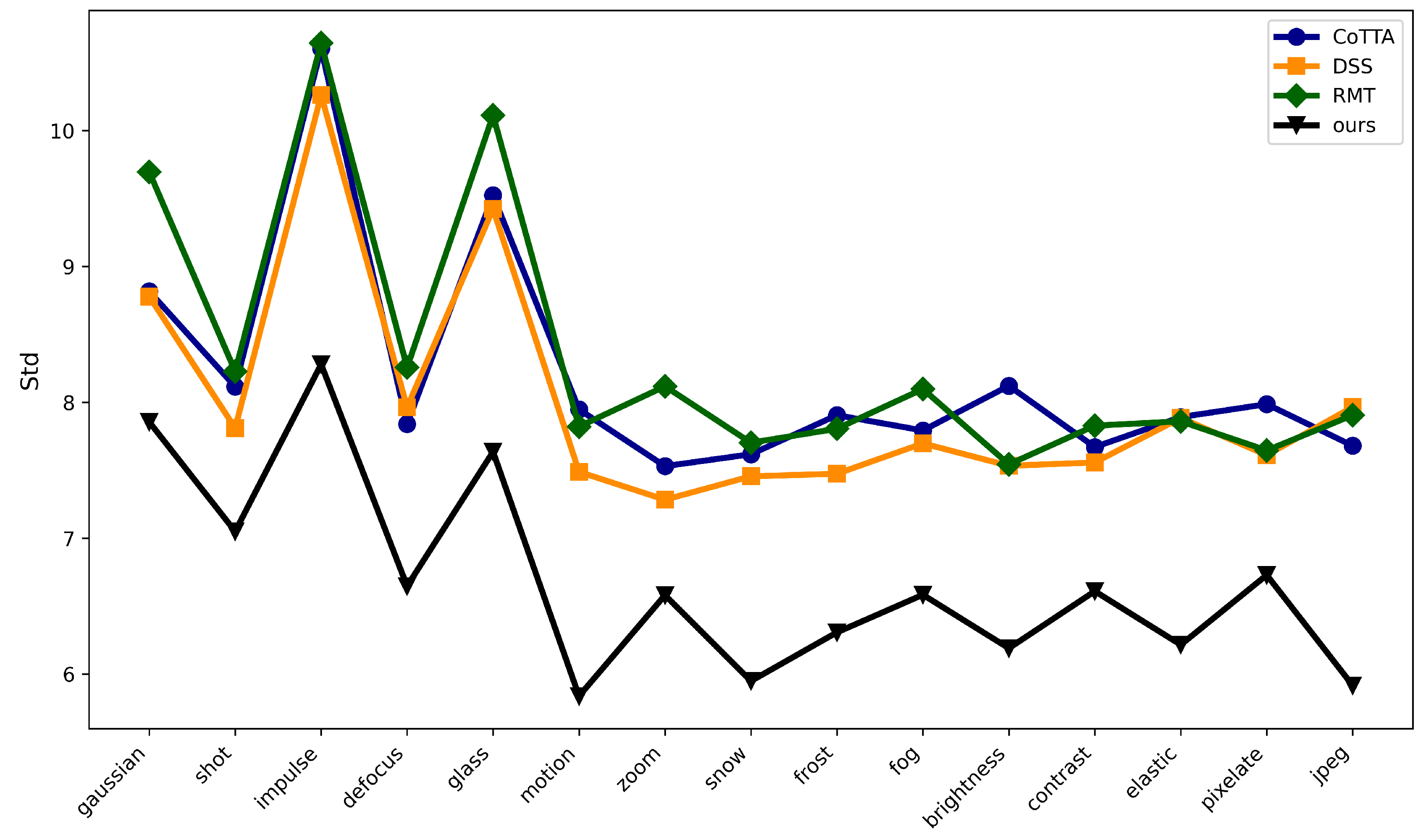
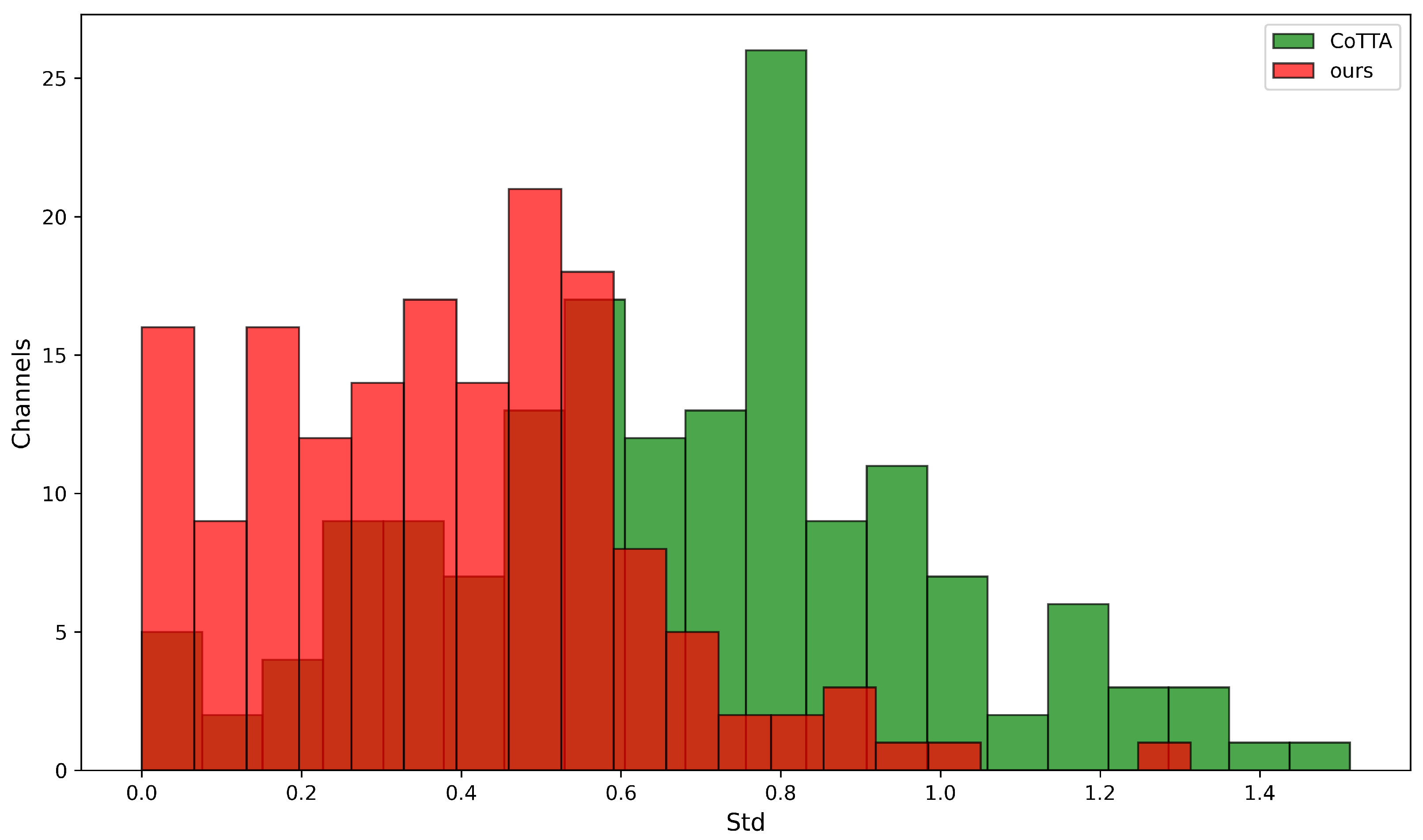
In this section, we focus on evaluating the effectiveness of Domain Sensitivity Parameter Suppression (DSP). The dataset used is CIFAR10C, and the pretrained network is WideResNet-28. The methods compared include CoTTA [5], DSS [8], and RMT [6]. First, we measure the model’s sensitivity to the domain by calculating the unstable representations of all channels in the network. The calculation formula is $St{d}_{channels}={\sum }_{l=0}^L{\sum }_{i=0}^{C^l}\sqrt{\parallel \widetilde{C_i^l}-C_i^l{\parallel }_2^2}$ where $\widetilde{C_i^l}$ represent the channel features generated by the source domain data in the target domain network, and $C_i^l$ represent the channel features generated by the target domain data in the target domain network. As shown in Figure 5, our method consistently achieves the lowest unstable activation values across all domains. This indicates that DSP effectively suppresses the learning of domain-specific knowledge by regulating the updates of domain-sensitive parameters. This, in turn, enhances the learning of domain-invariant knowledge and prevents the model from overfitting to current domain knowledge during continuous domain shifts, thereby mitigating interference with future domains that may be encountered. Furthermore, we examined the relationship between the number of channels in the first layer of the network and their corresponding unstable activation values. As shown in Figure 6, the unstable representations of DSP exhibit a smaller variance, with activation values concentrating around 0.35 across all channels. This demonstrates that the introduction of DSP can effectively control channel instability, enabling the model to maintain strong robustness and effectively counteract the effects of domain shifts.

Additionally, inspired by adversarial training, we incorporate an auxiliary discriminator network to evaluate the effectiveness of DSP in promoting the learning of domain-invariant representations. Specifically, we add a source domain discriminator to the first layer of the WideResNet-28 network and train this discriminator on the CIFAR-10 dataset. The source domain discriminator takes the output of the first layer as input and generates a score indicating the likelihood that the input belongs to the source domain. Intuitively, if the domain-sensitive parameters are effectively suppressed, the model’s output should remain highly robust and well aligned with the source domain, regardless of the domain shifts. As shown in Figure 7, compared with other methods on CIFAR10C, our approach consistently maintains high robustness to the source domain across all domains, indicating that the domain-sensitivity parameters have been effectively suppressed.

4.5. Analysis of Dynamic Virtual Margin

In this section, we focus on discussing the parameter initialization of the virtual decision margin m and the superiority of dynamic virtual margins. First, we explore the effects of different initialization values for the parameters on three datasets (CIFAR10C, CIFAR100C, ImageNetC). As shown in

Table 8. Performance results (error rate %) with different values of m on CIFAR10C, CIFAR100C, and ImageNetC datasets.

	m = 1	m = 2	m = 3	m = 4	m = 5	m = 6	m = 7	m = 8
CIFAR10C	14.8	14.5	14.7	14.9	15.3	15.5	16.1	16.8
CIFAR100C	27.9	27.8	28.2	28.3	28.4	28.7	29.5	30.1
ImageNetC	58.1	57.9	58.1	58.3	58.6	59.1	59.7	60.9

, the initialization of the virtual decision margin parameters is highly robust. When m is set between 1 and 6, it performs well across all three datasets. However, when m exceeds 6, the performance begins to gradually decline. This is because a larger virtual margin increases the difficulty of model convergence during the initial phase of domain adaptation, leading to a drop in performance. We recommend initializing with a smaller virtual margin, allowing the margin to adaptively adjust to an appropriate value to avoid convergence difficulties caused by a large margin in the early stages of adaptation.

Overall, the dynamic virtual margin can adaptively adjust the margin width based on domain and class difficulty, and is not sensitive to initialization parameters, showing good robustness with excellent performance across a broad initialization range.

Next, we investigate the performance of fixed and dynamic virtual margins. As shown in

Table 9. Performance results (error rate %) with different values of fixed m and dynamic m on CIFAR10C, CIFAR100C, and ImageNetC datasets.

	m = 1	m = 2	m = 3	m = 4	m = 5	m = 6	m = 7	m = 8	m = Dynamic
CIFAR10C	15.3	15.2	14.9	15.5	15.9	16.3	16.7	17.3	14.5
CIFAR100C	28.2	28.1	28.5	28.9	29.3	29.7	30.2	31.1	27.8
ImageNetC	58.7	58.2	58.5	58.9	59.3	59.9	60.3	61.2	57.9

, dynamic virtual margins outperform fixed virtual margins on all datasets. This is due to the dynamic margin’s ability to adaptively adjust the margin size based on domain and class difficulty, achieving optimal performance.

4.6. Analysis of Virtual Decision Boundary

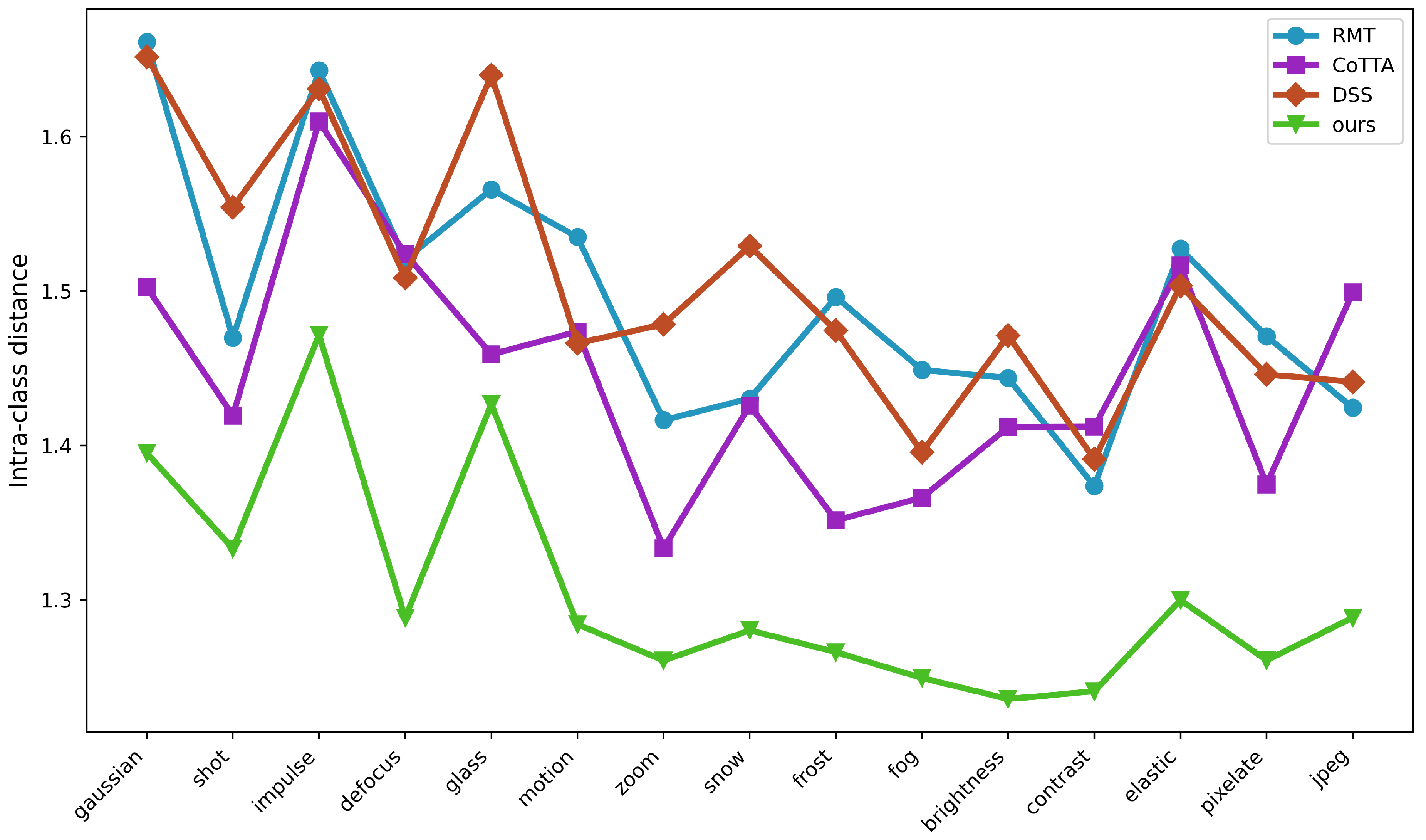
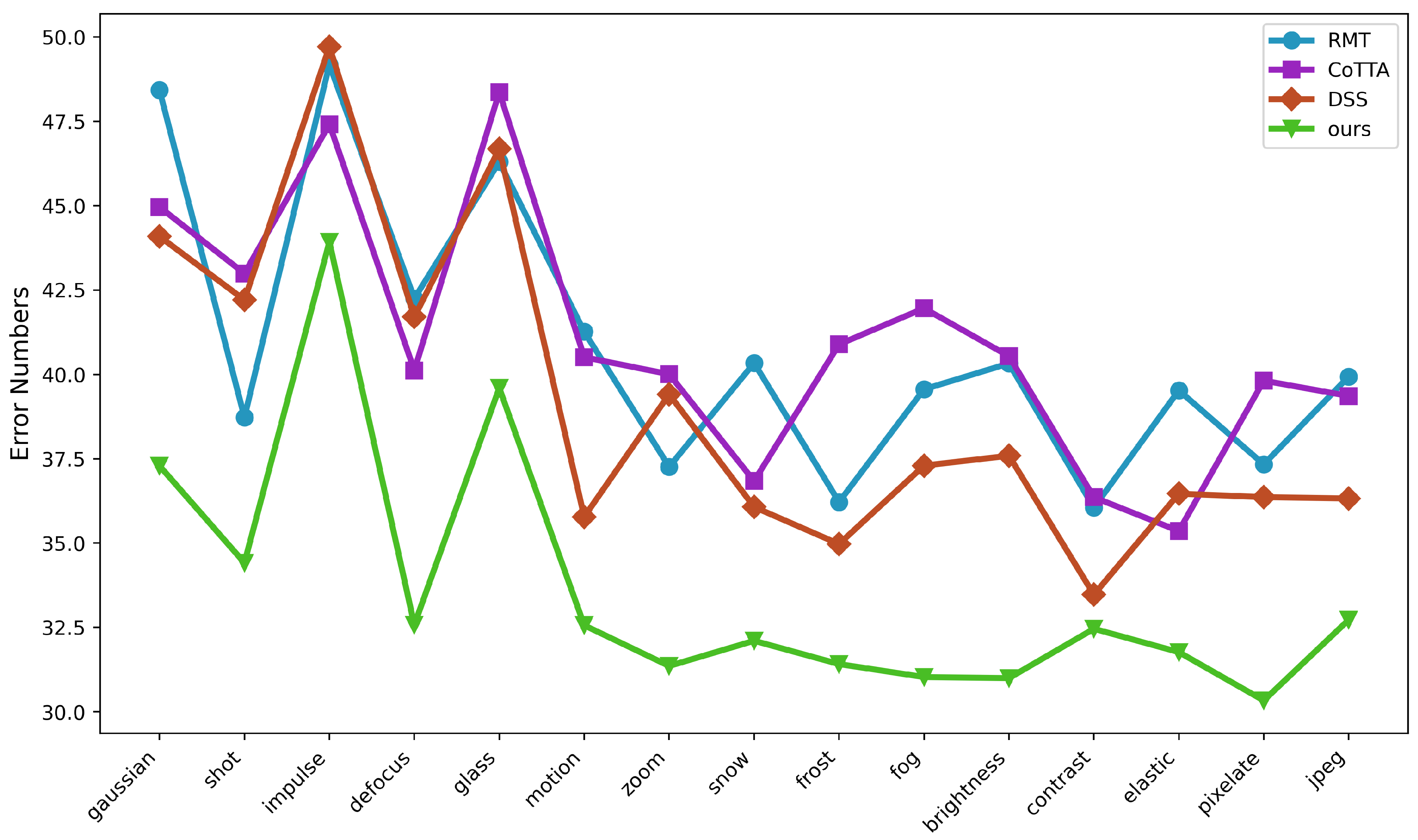
We evaluate the effectiveness of our virtual decision boundary (VDB) method in mitigating feature crossing the decision boundary by analyzing inter-class and intra-class distances. Our VDB method is proposed to alleviate the issue of feature clustering at or slightly crossing the decision boundary. First, we utilized T-SNE to visualize the sample features generated by three different methods (DSS [8], CoTTA [5], RMT [6]) and our method in the Gaussian domain of the CIFAR10C dataset. As shown in Figure 8, the results demonstrate that the features generated by our method exhibit better clustering performance, with smaller intra-class distances and larger inter-class distances. Second, if class feature shifts are well controlled, the inter-class distance should increase, and the intra-class distance should decrease. This will effectively prevent features from crossing the decision boundary. The intra-class distance is expressed as $d_{intra}={\sum }_i^C\left|\right|z_i-\overline{z_i}{\left|\right|}_2$, and the inter-class distance is expressed as $d_{inter}={\sum }_i^C{\sum }_{j\ne i}^C\left|\right|z_i-\overline{z_j}{\left|\right|}_2$, where $\overline{z}$ represents the mean feature of the class. As shown in Figure 9 and Figure 10, we compare our approach with three other methods include DSS [8], CoTTA [5], and RMT [44]. The results demonstrate that our method excels in managing class shifts during CTTA, consistently achieving more desirable intra-class and inter-class distances across all domains. In particular, to evaluate the effectiveness of our virtual decision boundary in mitigating feature crossing the decision boundary during the early stages of domain adaptation, we counted the number of features crossing the decision boundary for each method at the early stage of domain adaptation. As shown in Figure 11, our method consistently outperforms others across all domains.

4.7. Time and Parameter Complexity Evaluation

In this section, we focus on analyzing the time and space complexity of our method compared with other methods. The datasets used include CIFAR10C, CIFAR100C, and ImageNetC, and the methods for comparison include TENT [12], CoTTA [5], DSS [8], and RMT [6]. As shown in

Table 10. Time required for different methods on CIFAR10C, CIFAR100C, and ImageNetC datasets.

	TENT	CoTTA	DSS	RMT	Ours
CIFAR10C	7 min	15 min	16 min	15 min	19 min
CIFAR100C	9 min	17 min	19 min	18 min	23 min
ImageNetC	33 min	71 min	73 min	72 min	86 min

, the time required by our method is only 3 min, 4 min, and 13 min more than the most time-consuming DSS [8] method on the CIFAR10C, CIFAR100C, and ImageNetC datasets, respectively. The reason for the additional time consumption is that our method requires the computation of the channel feature map from the previous model (without computing gradients) and the calculation of the sensitivity loss function. As shown in Figure 12, compared with CoTTA [5], DSS [8], and RMT [6], our method requires more GPU memory at runtime, approximately 0.8GB, due to the additional storage of feature maps computed by the previous model. This additional time and space complexity overhead are small and can be largely ignored, which leads to significant performance improvements.

5. Conclusions

Distinguishing itself from previous research that tends to concentrate on isolated domain adaptation and seeks local optima. Instead, this paper focuses on the often overlooked sustained capability in Continual Test-Time Adaptation. To address this issue, we propose a Dual Constraint method that combines parameter constraints based on channel representations and virtual decision boundary constraints based on features. The parameter constraint penalizes the model’s reliance on domain-specific knowledge, forcing it to learn domain-invariant knowledge while alleviating channel instability and mutual interference caused by overfitting to domain-sensitive parameters. This approach also theoretically enhances the model’s generalization ability. Additionally, we provide theoretical evidence that our method can effectively enhance the model’s generalization ability and promote the learning of domain-invariant knowledge. Meanwhile, the virtual decision boundary constraint pushes features away from the original decision boundary, forming a virtual margin that buffers against domain shifts, effectively reducing the mutual interference between domain-specific knowledge. Our extensive experiments on multiple CTTA benchmark datasets have demonstrated the effectiveness of our proposed methods.

References

1. Hu, C.; Hudson, S.; Ethier, M.; Al-Sharman, M.; Rayside, D.; Melek, W. Sim-to-real domain adaptation for lane detection and classification in autonomous driving. In Proceedings of the 2022 IEEE Intelligent Vehicles Symposium (IV), Aachen, Germany, 4–9 June 2022; IEEE: New York, NY, USA, 2022; pp. 457–463. [Google Scholar]
2. Shi, Z.; Su, T.; Liu, P.; Wu, Y.; Zhang, L.; Wang, M. Learning Frequency-Aware Dynamic Transformers for All-In-One Image Restoration. arXiv 2024, arXiv:2407.01636. [Google Scholar] [CrossRef]
3. Chen, W.; Miao, L.; Gui, J.; Wang, Y.; Li, Y. FLsM: Fuzzy Localization of Image Scenes Based on Large Models. Electronics 2024, 13, 2106. [Google Scholar] [CrossRef]
4. Xu, E.; Zhu, J.; Zhang, L.; Wang, Y.; Lin, W. Research on Aspect-Level Sentiment Analysis Based on Adversarial Training and Dependency Parsing. Electronics 2024, 13, 1993. [Google Scholar] [CrossRef]
5. Wang, Q.; Fink, O.; Van Gool, L.; Dai, D. Continual test-time domain adaptation. In Proceedings of the IEEE/CVF Conference on Computer Vision and Pattern Recognition, New Orleans, LA, USA, 18–24 June 2022; pp. 7201–7211. [Google Scholar]
6. Döbler, M.; Marsden, R.A.; Yang, B. Robust mean teacher for continual and gradual test-time adaptation. In Proceedings of the IEEE/CVF Conference on Computer Vision and Pattern Recognition, Vancouver, BC, Canada, 17–24 June 2023; pp. 7704–7714. [Google Scholar]
7. Brahma, D.; Rai, P. A probabilistic framework for lifelong test-time adaptation. In Proceedings of the IEEE/CVF Conference on Computer Vision and Pattern Recognition, Vancouver, BC, Canada, 17–24 June 2023; pp. 3582–3591. [Google Scholar]
8. Wang, Y.; Hong, J.; Cheraghian, A.; Rahman, S.; Ahmedt-Aristizabal, D.; Petersson, L.; Harandi, M. Continual test-time domain adaptation via dynamic sample selection. In Proceedings of the IEEE/CVF Winter Conference on Applications of Computer Vision, Waikoloa, HI, USA, 3–8 January 2024; pp. 1701–1710. [Google Scholar]
9. Liu, J.; Yang, S.; Jia, P.; Zhang, R.; Lu, M.; Guo, Y.; Xue, W.; Zhang, S. Vida: Homeostatic visual domain adapter for continual test time adaptation. arXiv 2023, arXiv:2306.04344. [Google Scholar]
10. Zhu, Z.; Hong, X.; Ma, Z.; Zhuang, W.; Ma, Y.; Dai, Y.; Wang, Y. Reshaping the Online Data Buffering and Organizing Mechanism for Continual Test-Time Adaptation. In Proceedings of the European Conference on Computer Vision, Dublin, Ireland, 22–23 October 2025; Springer: Berlin/Heidelberg, Germany, 2025; pp. 415–433. [Google Scholar]
11. Liu, J.; Xu, R.; Yang, S.; Zhang, R.; Zhang, Q.; Chen, Z.; Guo, Y.; Zhang, S. Continual-MAE: Adaptive Distribution Masked Autoencoders for Continual Test-Time Adaptation. In Proceedings of the IEEE/CVF Conference on Computer Vision and Pattern Recognition, Seattle, WA, USA, 16–22 June 2024; pp. 28653–28663. [Google Scholar]
12. Wang, D.; Shelhamer, E.; Liu, S.; Olshausen, B.; Darrell, T. Tent: Fully test-time adaptation by entropy minimization. arXiv 2020, arXiv:2006.10726. [Google Scholar]
13. DeVore, R.A.; Temlyakov, V.N. Some remarks on greedy algorithms. Adv. Comput. Math. 1996, 5, 173–187. [Google Scholar] [CrossRef]
14. Knowles, J.D.; Watson, R.A.; Corne, D.W. Reducing local optima in single-objective problems by multi-objectivization. In Proceedings of the International Conference on Evolutionary Multi-Criterion Optimization, Zurich, Switzerland, 7–9 March 2001; Springer: Berlin/Heidelberg, Germany, 2001; pp. 269–283. [Google Scholar]
15. Wang, D.Z.; Lo, H.K. Global optimum of the linearized network design problem with equilibrium flows. Transp. Res. Part B Methodol. 2010, 44, 482–492. [Google Scholar] [CrossRef]
16. Zhou, W.; Zhou, Z. Unsupervised Domain Adaption Harnessing Vision-Language Pre-Training. IEEE Trans. Circuits Syst. Video Technol. 2024, 34, 8201–8214. [Google Scholar] [CrossRef]
17. Wilson, G.; Cook, D.J. A survey of unsupervised deep domain adaptation. ACM Trans. Intell. Syst. Technol. (Tist) 2020, 11, 1–46. [Google Scholar] [CrossRef]
18. Long, M.; Cao, Y.; Wang, J.; Jordan, M. Learning transferable features with deep adaptation networks. In Proceedings of the International Conference on Machine Learning, Lille, France, 6–11 July 2015; PMLR: San Diego, CA, USA, 2015; pp. 97–105. [Google Scholar]
19. Long, M.; Zhu, H.; Wang, J.; Jordan, M.I. Unsupervised domain adaptation with residual transfer networks. Adv. Neural Inf. Process. Syst. 2016, 29. [Google Scholar]
20. Long, M.; Zhu, H.; Wang, J.; Jordan, M.I. Deep transfer learning with joint adaptation networks. In Proceedings of the International Conference on Machine Learning, Sydney, Australia, 6–11 August 2017; PMLR: San Diego, CA, USA, 2017; pp. 2208–2217. [Google Scholar]
21. Fan, X.; Wang, Q.; Ke, J.; Yang, F.; Gong, B.; Zhou, M. Adversarially adaptive normalization for single domain generalization. In Proceedings of the IEEE/CVF Conference on Computer Vision and Pattern Recognition, Nashville, TN, USA, 20–25 June 2021; pp. 8208–8217. [Google Scholar]
22. Yang, F.E.; Cheng, Y.C.; Shiau, Z.Y.; Wang, Y.C.F. Adversarial teacher-student representation learning for domain generalization. Adv. Neural Inf. Process. Syst. 2021, 34, 19448–19460. [Google Scholar]
23. Zhu, W.; Lu, L.; Xiao, J.; Han, M.; Luo, J.; Harrison, A.P. Localized adversarial domain generalization. In Proceedings of the IEEE/CVF Conference on Computer Vision and Pattern Recognition, New Orleans, LA, USA, 18–24 June 2022; pp. 7108–7118. [Google Scholar]
24. Liang, J.; Hu, D.; Feng, J. Do we really need to access the source data? source hypothesis transfer for unsupervised domain adaptation. In Proceedings of the International Conference on Machine Learning, Virtual, 13–18 July 2020; PMLR: San Diego, CA, USA, 2020; pp. 6028–6039. [Google Scholar]
25. Lowd, D.; Meek, C. Adversarial learning. In Proceedings of the Eleventh ACM SIGKDD International Conference on Knowledge Discovery in Data Mining, Chicago, IL, USA, 21–24 August 2005; pp. 641–647. [Google Scholar]
26. Gopnik, A.; Glymour, C.; Sobel, D.M.; Schulz, L.E.; Kushnir, T.; Danks, D. A theory of causal learning in children: Causal maps and Bayes nets. Psychol. Rev. 2004, 111, 3. [Google Scholar] [CrossRef] [PubMed]
27. Hospedales, T.; Antoniou, A.; Micaelli, P.; Storkey, A. Meta-learning in neural networks: A survey. IEEE Trans. Pattern Anal. Mach. Intell. 2021, 44, 5149–5169. [Google Scholar] [CrossRef] [PubMed]
28. Cubuk, E.D.; Zoph, B.; Shlens, J.; Le, Q.V. Randaugment: Practical automated data augmentation with a reduced search space. In Proceedings of the IEEE/CVF conference on Computer Vision and Pattern Recognition Workshops, Seattle, WA, USA, 14–19 June 2020; pp. 702–703. [Google Scholar]
29. Zhou, K.; Yang, Y.; Hospedales, T.; Xiang, T. Deep domain-adversarial image generation for domain generalisation. In Proceedings of the AAAI Conference on Artificial Intelligence, New York, NY, USA, 7–12 February 2020; Volume 34, pp. 13025–13032. [Google Scholar]
30. Gan, Y.; Bai, Y.; Lou, Y.; Ma, X.; Zhang, R.; Shi, N.; Luo, L. Decorate the newcomers: Visual domain prompt for continual test time adaptation. In Proceedings of the AAAI Conference on Artificial Intelligence, Washington, DC, USA, 7–14 February 2023; Volume 37, pp. 7595–7603. [Google Scholar]
31. Wang, H.; Ge, S.; Lipton, Z.; Xing, E.P. Learning robust global representations by penalizing local predictive power. Adv. Neural Inf. Process. Syst. 2019, 32. [Google Scholar]
32. Guo, J.; Qi, L.; Shi, Y. Domaindrop: Suppressing domain-sensitive channels for domain generalization. In Proceedings of the IEEE/CVF International Conference on Computer Vision, Paris, France, 2–3 October 2023; pp. 19114–19124. [Google Scholar]
33. Zhao, Y.; Zhang, H.; Hu, X. Penalizing gradient norm for efficiently improving generalization in deep learning. In Proceedings of the International Conference on Machine Learning, Baltimore, MD, USA, 17–23 July 2022; PMLR: San Diego, CA, USA, 2022; pp. 26982–26992. [Google Scholar]
34. Cong, W.; Cong, Y.; Sun, G.; Liu, Y.; Dong, J. Self-Paced Weight Consolidation for Continual Learning. IEEE Trans. Circuits Syst. Video Technol. 2024, 34, 2209–2222. [Google Scholar] [CrossRef]
35. Zhang, W.; Huang, Y.; Zhang, W.; Zhang, T.; Lao, Q.; Yu, Y.; Zheng, W.S.; Wang, R. Continual Learning of Image Classes With Language Guidance From a Vision-Language Model. IEEE Trans. Circuits Syst. Video Technol. 2024, 34, 13152–13163. [Google Scholar] [CrossRef]
36. Yu, D.; Zhang, M.; Li, M.; Zha, F.; Zhang, J.; Sun, L.; Huang, K. Contrastive Correlation Preserving Replay for Online Continual Learning. IEEE Trans. Circuits Syst. Video Technol. 2024, 34, 124–139. [Google Scholar] [CrossRef]
37. Li, H.; Liao, L.; Chen, C.; Fan, X.; Zuo, W.; Lin, W. Continual Learning of No-Reference Image Quality Assessment With Channel Modulation Kernel. IEEE Trans. Circuits Syst. Video Technol. 2024, 34, 13029–13043. [Google Scholar] [CrossRef]
38. Li, K.; Chen, H.; Wan, J.; Yu, S. ESDB: Expand the Shrinking Decision Boundary via One-to-Many Information Matching for Continual Learning With Small Memory. IEEE Trans. Circuits Syst. Video Technol. 2024, 34, 7328–7343. [Google Scholar] [CrossRef]
39. Shi, Z.; Liu, P.; Su, T.; Wu, Y.; Liu, K.; Song, Y.; Wang, M. Densely Distilling Cumulative Knowledge for Continual Learning. arXiv 2024, arXiv:2405.09820. [Google Scholar] [CrossRef]
40. Wu, Y.; Chi, Z.; Wang, Y.; Plataniotis, K.N.; Feng, S. Test-time domain adaptation by learning domain-aware batch normalization. In Proceedings of the AAAI Conference on Artificial Intelligence, Philadelphia, PA, USA, 25 February–4 March; Volume 38, pp. 15961–15969.
41. Zhang, J.; Qi, L.; Shi, Y.; Gao, Y. Domainadaptor: A novel approach to test-time adaptation. In Proceedings of the IEEE/CVF International Conference on Computer Vision, Paris, France, 2–3 October 2023; pp. 18971–18981. [Google Scholar]
42. Chen, K.; Gong, T.; Zhang, L. Camera-Aware Recurrent Learning and Earth Mover’s Test-Time Adaption for Generalizable Person Re-Identification. IEEE Trans. Circuits Syst. Video Technol. 2024, 34, 357–370. [Google Scholar] [CrossRef]
43. Wang, Y.; Chen, H.; Heng, Q.; Hou, W.; Fan, Y.; Wu, Z.; Wang, J.; Savvides, M.; Shinozaki, T.; Raj, B.; et al. Freematch: Self-adaptive thresholding for semi-supervised learning. arXiv 2022, arXiv:2205.07246. [Google Scholar]
44. Yuan, L.; Xie, B.; Li, S. Robust test-time adaptation in dynamic scenarios. In Proceedings of the IEEE/CVF Conference on Computer Vision and Pattern Recognition, Vancouver, BC, Canada, 17–24 June 2023; pp. 15922–15932. [Google Scholar]
45. Shi, B.; Zhang, D.; Dai, Q.; Zhu, Z.; Mu, Y.; Wang, J. Informative dropout for robust representation learning: A shape-bias perspective. In Proceedings of the International Conference on Machine Learning, Virtual, 13–18 July 2020; PMLR: San Diego, CA, USA, 2020; pp. 8828–8839. [Google Scholar]
46. Klinker, F. Exponential moving average versus moving exponential average. Math. Semesterber. 2011, 58, 97–107. [Google Scholar]
47. Dinh, L.; Pascanu, R.; Bengio, S.; Bengio, Y. Sharp minima can generalize for deep nets. In Proceedings of the International Conference on Machine Learning, Sydney, Australia, 6–11 August 2017; PMLR: San Diego, CA, USA, 2017; pp. 1019–1028. [Google Scholar]
48. Yang, S.; Wu, J.; Liu, J.; Li, X.; Zhang, Q.; Pan, M.; Zhang, S. Exploring sparse visual prompt for cross-domain semantic segmentation. arXiv 2023, arXiv:2303.09792. [Google Scholar]
49. Sakaridis, C.; Dai, D.; Van Gool, L. ACDC: The adverse conditions dataset with correspondences for semantic driving scene understanding. In Proceedings of the IEEE/CVF International Conference on Computer Vision, Montreal, QC, Canada, 10–17 October 2021; pp. 10765–10775. [Google Scholar]
50. Li, Y.; Wang, N.; Shi, J.; Liu, J.; Hou, X. Revisiting batch normalization for practical domain adaptation. arXiv 2016, arXiv:1603.04779. [Google Scholar] [CrossRef]
51. Chakrabarty, G.; Sreenivas, M.; Biswas, S. Sata: Source anchoring and target alignment network for continual test time adaptation. arXiv 2023, arXiv:2304.10113. [Google Scholar] [CrossRef]
52. Zagoruyko, S.; Komodakis, N. Wide residual networks. arXiv 2016, arXiv:1605.07146. [Google Scholar]
53. Xie, S.; Girshick, R.; Dollár, P.; Tu, Z.; He, K. Aggregated residual transformations for deep neural networks. In Proceedings of the IEEE Conference on Computer Vision and Pattern Recognition, Honolulu, HI, USA, 21–26 July 2017; pp. 1492–1500. [Google Scholar]
54. He, K.; Zhang, X.; Ren, S.; Sun, J. Deep residual learning for image recognition. In Proceedings of the IEEE Conference on Computer Vision and Pattern Recognition, Las Vegas, NV, USA, 26 June–1 July 2016; pp. 770–778. [Google Scholar]
Figure 1. An illustration of the relationship between channels and unstable representations: (a) The instability of channel representations increases with the level of corruption. This indicates that domain shifts impact the channel outputs, and the stronger the domain shift, the greater the instability of the channel outputs. (b) The instability of representations varies across different channels. Domain-robust channels exhibit stable representations with smaller variance, typically concentrated on the left, suggesting that these channels have learned more domain-invariant knowledge, making them resilient to data distribution shifts and less prone to changes. In contrast, domain-sensitive channels show unstable representations with larger variance, typically concentrated on the right, as they have learned domain-specific knowledge, making them vulnerable to data distribution shifts and more susceptible to changes.
Electronics 14 03891 g001
Figure 2. Decision boundary lacks constraints. Consider a domain shift occurring between two adjacent time points, t and t + 1 . Features that are clustered near the decision boundary at time t are subjected to a stronger domain shift, causing them to cross the decision boundary and manifest as features at time t + 1 .
Electronics 14 03891 g002
Figure 3. Gradient norm and channel-unstable representation relationship.
Electronics 14 03891 g003
Figure 4. An illustrative example showcasing our motivation and solution: (a) During continuous domain adaptation, features are prone to cluster around or cross the decision boundary. (b) During domain shifts, features clustered at the decision boundary are prone to crossing it. (c) The virtual decision boundary forces the generated features away from the original decision boundary, creating a virtual margin that prevents features from crossing the decision boundary during domain shifts.
Electronics 14 03891 g004
Figure 5. Channels std in all domains.
Electronics 14 03891 g005
Figure 6. Channels std in first layer.
Electronics 14 03891 g006
Figure 7. Domain robustness score.
Electronics 14 03891 g007
Figure 8. Visualization on the Gaussian domain of the CIFAR10C dataset.
Electronics 14 03891 g008
Figure 9. Intra-class distance in all domains.
Electronics 14 03891 g009
Figure 10. Inter-class distance in all domains.
Electronics 14 03891 g010
Figure 11. Error numbers at the domain begin.
Electronics 14 03891 g011
Figure 12. Memory usage for different methods on various datasets.
Electronics 14 03891 g012