A Lithium-Ion Battery Remaining Useful Life Prediction Method Based on Mode Decomposition and Informer-LSTM

Abstract

To address the challenge of reduced prediction accuracy caused by capacity regeneration during the use of lithium-ion batteries, this study proposes an RUL (remaining useful life) prediction method based on mode decomposition and an enhanced Informer-LSTM hybrid model. The capacity is selected as the health indicator, and the CEEMDAN (complete ensemble empirical mode decomposition with adaptive noise) algorithm is employed to decompose the capacity sequence into high-frequency and low-frequency components. The high-frequency components are further decomposed and predicted using the Informer model, while the low-frequency components are predicted with an LSTM (long short-term memory) network. Pearson correlation coefficients between each component and the original sequence are calculated to determine fusion weights. The final RUL prediction is obtained through weighted integration of the individual predictions. Experimental validation on publicly available NASA and CALCE (Center for Advanced Life Cycle Engineering) battery datasets demonstrates that the proposed method achieves an average fitting accuracy of approximately 99%, with MAE (mean absolute error) below 0.02. Additionally, both MAPE (mean absolute percentage error) and RMSE (root-mean-square error) remain at low levels, indicating improvements in prediction precision.

1. Introduction

In recent years, renewable energy has attracted considerable attention due to the growing global energy demand and the worsening impacts of climate change [1,2]. Lithium-ion batteries, known for their high energy density, long cycle life, and environmental friendliness [3], are widely used in energy storage systems [4], electric vehicles [5], and aerospace applications [6]. However, as charge–discharge cycles accumulate, performance degradation becomes inevitable, typically manifested as gradual capacity fade and reduced power output, ultimately leading to end-of-life failure. If not replaced promptly, failed lithium-ion batteries may cause system malfunctions or physical damage, posing serious risks such as fire, explosion, and threats to human safety [7,8]. Therefore, accurate prediction of remaining useful life (RUL) is essential to ensuring system reliability and the protection of life and property [9,10].

Currently, lithium-ion battery RUL prediction mainly follows two approaches: model-based methods and data-driven methods [11]. Model-based approaches predict RUL by constructing mathematical representations of internal physicochemical mechanisms [12]. These models are generally classified into three types: equivalent circuit models [13,14], electrochemical models [15,16], and empirical degradation models [17,18].

Model-based methods can capture the degradation mechanisms of lithium-ion batteries in a physically interpretable manner. However, they often involve complex modeling procedures and require internal parameters that are difficult to obtain directly [19]. Consequently, data-driven approaches have gained popularity with the rapid development of machine learning and artificial intelligence. These approaches use machine learning or deep learning models to extract degradation features from historical data and construct mappings between these features and RUL. Wei et al. [20] combined the time warp profile (TWP) technique with support vector regression (SVR) to estimate the state of health (SOH) of lithium-ion batteries. Jin et al. [21] proposed an improved grey wolf optimization (IGWO) algorithm to optimize support vector machines (SVMs), achieving enhanced prediction performance.

Machine learning has achieved significant progress in battery life prediction. However, it still faces challenges in capturing long-range temporal dependencies and representing complex nonlinear dynamics in time-series data. Deep learning models, including convolutional neural network (CNN), long short-term memory (LSTM) network, and Transformer, have demonstrated improved accuracy and robustness due to their superior temporal modeling and automatic feature extraction capabilities. Compared with traditional machine learning models, CNNs can learn complex nonlinear mappings through stacked convolutional layers and are particularly effective in processing high-dimensional data. However, their use of fixed-size filters limits their ability to model long-range dependencies. As a result, CNNs tend to focus on recent data while neglecting long-term historical information. To address this limitation, a CNN is often combined with other models. Feng et al. [22] combined a CNN with bidirectional long short-term memory (BiLSTM) networks to incorporate both past and future contextual information, thus improving prediction accuracy. Jia et al. [23] developed a hybrid method combining a CNN with deep BiLSTM networks for RUL prediction, effectively mitigating performance degradation caused by limited training data. While LSTM networks are capable of learning temporal dynamics, their recursive computation makes them inefficient for modeling very long sequences and prone to gradient vanishing, resulting in slow training. In contrast, a Transformer [24] leverages self-attention mechanisms to enable parallel computation and capture global temporal features more effectively. Chen et al. [25] employed a denoising autoencoder (DAE) to preprocess raw data and fed the reconstructed sequences into a Transformer network, achieving improved prediction performance.

The capacity of a lithium-ion battery is a key indicator of its energy storage potential and discharge performance. In practical applications, temporary increases in capacity may occur due to factors such as material aging, thickening of the solid electrolyte interphase (SEI) layer, and loss of active material. These fluctuations can interfere with accurate life prediction. To reduce their influence, mode decomposition methods are employed to decompose the raw capacity degradation signal into several intrinsic mode functions (IMFs), each representing a distinct frequency component. This process effectively filters out short-term fluctuations and noise. Meng et al. [26] applied empirical mode decomposition (EMD) to the capacity sequence and used the resulting residual components as inputs to a particle filtering algorithm, thereby enhancing the accuracy of early-stage remaining useful life prediction. However, EMD is sensitive to noise and prone to mode mixing. To address these issues, Torres et al. [27] introduced the complete ensemble empirical mode decomposition with adaptive noise (CEEMDAN). By adding adaptive white noise during each decomposition and averaging multiple results, CEEMDAN effectively mitigates noise interference and alleviates mode mixing. Based on this method, Liu Bin et al. [28] proposed a prediction model that combines CEEMDAN with a BiLSTM-Transformer network, which proved effective in improving the precision of RUL prediction for lithium-ion batteries.

The analysis of the existing literature indicates that deep learning has been widely applied to lithium-ion battery life prediction. However, several limitations remain in the current research on lithium-ion battery life prediction. First, the IMF components can be broadly classified into high-frequency and low-frequency components. High-frequency components exhibit rapid and intense oscillations, while low-frequency components change more smoothly and reflect long-term trends. Most current approaches use a unified prediction model for all components, which often neglects their distinct characteristics; second, Transformer-based networks are capable of capturing long-range dependencies, making them suitable for handling high-frequency components. However, they often struggle with local feature variations and involve high computational costs. Last, not all decomposed components contribute equally to capacity degradation; some carry key information, while others mainly represent noise or short-term fluctuations. A simplistic fusion strategy limits the ability to accurately quantify the contribution of each component, thereby restricting overall predictive performance.

To address the aforementioned challenges, this study proposes a CEEMDAN-DInformer (Decomposition Informer)-LSTM framework for predicting the RUL of lithium-ion batteries. First, the capacity sequence is decomposed into multiple IMFs and a residual component using the CEEMDAN algorithm. The Pearson correlation coefficient is then employed to calculate the importance weight of each component relative to the original sequence. For high-frequency components, the DLinear decomposition strategy is applied to further separate each component into a trend term and a residual term. These subcomponents are independently predicted using the Informer model, and their sum is taken as the final prediction for each high-frequency component. Low-frequency components are directly predicted using an LSTM network. Finally, all component predictions are combined through a weighted summation based on their importance scores to generate the overall RUL prediction.

2. Basic Algorithm Theory

2.1. Complete Ensemble Empirical Mode Decomposition with Adaptive Noise

CEEMDAN, proposed by Torres et al., is an enhanced variant of the EMD algorithm. While EMD can decompose signals into multiple IMFs, it constructs envelope curves based on local extrema, which may lead to mode mixing—where signal components from different frequency bands are combined within a single IMF. This issue is especially pronounced when handling signals that exhibit complex temporal characteristics, ultimately reducing prediction accuracy.

CEEMDAN mitigates this problem by adding adaptive white noise during the computation of each IMF. This process enhances the statistical independence among components, effectively mitigates mode mixing, and reduces reconstruction error. As a result, CEEMDAN enables more accurate multi-scale decomposition, effectively isolating meaningful signal features and mitigating the adverse effects of capacity regeneration on prediction performance. The CEEMDAN algorithm consists of the following key steps:

• (1) Add a white noise sequence, drawn from a Gaussian distribution, to the original capacity sequence:

$${\mathrm{X}}_{\mathrm{i}}(\mathrm{t})=\mathrm{X}(\mathrm{t})+{\mathsf{\epsilon }}_0{\mathsf{\omega }}_{\mathrm{i}}(\mathrm{t})$$

(1)

where ε₀ denotes the signal-to-noise ratio, and ω_i represents the white noise sequence.

• (2) Perform EMD on the noise-enhanced sequence X_i(t). Then, compute the average of the resulting decompositions to obtain IMF₁ and the first residual sequence:

$${\mathrm{IMF}}_1={\displaystyle \frac{1}{ \mathrm{N}}}{\displaystyle \sum _{\mathrm{i}=1}^{\mathrm{N}}\mathrm{EMD}}\left({\mathrm{X}}_{\mathrm{i}}(\mathrm{t})\right)$$

(2)

$${\mathrm{R}}_1(\mathrm{t})=\mathrm{X}(\mathrm{t})-{\mathrm{IMF}}_1$$

(3)

(3) Add white noise to the first residual sequence R₁(t) obtained in step (2), and perform EMD again to extract IMF₂ and the updated residual sequence:

$${\mathrm{R}}_1^{\mathrm{i}}(\mathrm{t})={\mathrm{R}}_1(\mathrm{t})+{\mathsf{\epsilon }}_1{\mathsf{\omega }}_{\mathrm{i}}(\mathrm{t})$$

(4)

$${\mathrm{IMF}}_2={\displaystyle \frac{1}{ \mathrm{N}}}{\displaystyle \sum _{\mathrm{i}=1}^{\mathrm{N}}\mathrm{EMD}}\left({\mathrm{R}}_1^{\mathrm{i}}(\mathrm{t})\right)$$

(5)

$${\mathrm{R}}_2\left(\mathrm{t}\right)={\mathrm{R}}_1\left(\mathrm{t}\right)-{\mathrm{IMF}}_2$$

(6)

where ε_i denotes the signal-to-noise ratio, which is adaptively adjusted to meet the requirements of the current decomposition stage.

• (4) This procedure is repeated to extract successive IMFs and terminates when the residual sequence becomes a monotonic function:

$${\mathrm{IMF}}_{\mathrm{k}}={\displaystyle \frac{1}{ \mathrm{N}}}{\displaystyle \sum _{\mathrm{i}=1}^{\mathrm{N}}\mathrm{EMD}}\left({\mathrm{R}}_{\mathrm{k}-1}^{\mathrm{i}}(\mathrm{t})\right)$$

(7)

$${\mathrm{R}}_{\mathrm{k}}\left(\mathrm{t}\right)={\mathrm{R}}_{\mathrm{k}-\mathrm{1}}\left(\mathrm{t}\right)-{\mathrm{IMF}}_{\mathrm{k}}$$

(8)

(5) After CEEMDAN decomposition, the original signal can be represented as:

$${\mathrm{X}\left(\mathrm{t}\right)=\mathrm{R}}_{\mathrm{n}}\left(\mathrm{t}\right)+{\displaystyle \sum _{\mathrm{i}=1}^{\mathrm{n}}\mathrm{I}}{\mathrm{MF}}_{\mathrm{i}}$$

(9)

2.2. Pearson Correlation Coefficient

Originally introduced by the British statistician Karl Pearson in the late 19th century, the Pearson correlation coefficient remains a widely used statistical measure for quantifying the linear relationship between two variables. In statistics, covariance is commonly used to evaluate the relationship between variables. However, covariance is influenced by the scale of the data and does not reflect relative trends. To address this, covariance is normalized to remove the effect of the data scale. The calculation is given by the following formula:

$$\mathrm{r}={\displaystyle \frac{{\displaystyle \sum _{\mathrm{i}=1}^{\mathrm{n}}\left({\mathrm{x}}_{\mathrm{i}}-\overline{\mathrm{x}}\right)}\left({\mathrm{y}}_{\mathrm{i}}-\overline{\mathrm{y}}\right)}{\sqrt{{\displaystyle \sum _{\mathrm{i}=1}^{\mathrm{n}}{\left({\mathrm{x}}_{\mathrm{i}}-\overline{\mathrm{x}}\right)}^2}}\sqrt{{\displaystyle \sum _{\mathrm{i}=1}^{\mathrm{n}}{\left({\mathrm{y}}_{\mathrm{i}}-\overline{\mathrm{y}}\right)}^2}}}}$$

(10)

In this equation, x and y represent the two variables, and r denotes the computed correlation coefficient. A larger absolute value of r indicates a stronger linear relationship between the variables.

After decomposing the original capacity signal into multiple IMFs, each IMF captures signal characteristics at a specific frequency. Some IMFs contain key information related to capacity degradation, while others mainly reflect noise or weakly correlated components. Consequently, the contribution of each IMF to the overall capacity trend varies. Directly summing all IMFs may result in substantial prediction errors. To address this issue, the Pearson correlation coefficient is used to quantify the relevance of each IMF to the original signal and to assign corresponding weights for weighted integration.

2.3. Long Short-Term Memory Network

LSTM was developed to address the issues of gradient vanishing and explosion commonly found in recurrent neural networks (RNNs). By incorporating gating mechanism, LSTM can effectively manage long-range dependencies in sequential data. The structure of a typical LSTM unit is illustrated in Figure 1.

LSTM units consist of three main gates: the forget gate, the input gate, and the output gate.

The forget gate determines which information from the previous cell state C_t−1 should be discarded and is calculated as follows:

$${\mathrm{f}}_{\mathrm{t}}=\mathsf{\sigma }\left({\mathrm{W}}_{\mathrm{f}}\left[{\mathrm{h}}_{\mathrm{t}-1}{,\mathrm{x}}_{\mathrm{t}}\right]{+\mathrm{b}}_{\mathrm{f}}\right)$$

(11)

The symbol σ represents the sigmoid activation function; W_f and b_f denote the weights and biases of the forget gate, respectively; h_t−1 is the hidden state from the previous time step; and x_t is the input at the current time step.

The input gate regulates the addition of new information to the cell state by identifying important data. It selectively updates the previous cell state with important information to form the current state. The calculation process is as follows:

$${\mathrm{i}}_{\mathrm{t}}=\mathsf{\sigma }\left({\mathrm{W}}_{\mathrm{i}}\left[{\mathrm{h}}_{\mathrm{t}-1}{,\mathrm{x}}_{\mathrm{t}}\right]{+\mathrm{b}}_{\mathrm{i}}\right)$$

(12)

$${\overline{\mathrm{C}}}_{\mathrm{t}}=\tanh \left({\mathrm{W}}_{\mathrm{C}}\left[{\mathrm{h}}_{\mathrm{t}-1}{,\mathrm{x}}_{\mathrm{t}}\right]{+\mathrm{b}}_{\mathrm{C}}\right)$$

(13)

$${\mathrm{C}}_{\mathrm{t}}{=\mathrm{f}}_{\mathrm{t}}{·\mathrm{C}}_{\mathrm{t}-1}{+\mathrm{i}}_{\mathrm{t}}·{\overline{\mathrm{C}}}_{\mathrm{t}}$$

(14)

where i_t is the activation value of the input gate, generated based on the previous hidden state h_t−1 and the current input x_t; $\overline{C}$_t is the candidate cell state, representing the new information that may be added to the cell state at the current time step, generated through the tanh activation function; and C_t is the updated cell state after incorporating the new information.

The output gate regulates the current hidden state h_t−1, determining which information is transmitted to the next layer. The computation is given by:

$${\mathrm{O}}_{\mathrm{t}}=\mathsf{\sigma }\left({\mathrm{W}}_{\mathrm{O}}\left[{\mathrm{h}}_{\mathrm{t}-1}{,\mathrm{X}}_{\mathrm{t}}\right]{+\mathrm{b}}_{\mathrm{O}}\right)$$

(15)

$${\mathrm{h}}_{\mathrm{t}}{=\mathrm{O}}_{\mathrm{t}}·\tanh \left({\mathrm{C}}_{\mathrm{t}}\right)$$

(16)

where O_t indicates the degree to which input information is retained at the current time step, with values closer to 1 signifying higher retention; and C_t represents the cell state at the current time step and is used to compute the hidden state h_t, which is passed to the next layer.

Compared with traditional statistical models, long short-term memory networks provide higher accuracy in modeling sequences with relatively smooth variations. However, they tend to respond slowly to abrupt short-term changes and perform less effectively on sequences characterized by frequent and intense fluctuations. Consequently, LSTM networks are better suited for modeling low-frequency components, such as the residual sequences obtained through CEEMDAN decomposition.

2.4. Informer

Although Transformer performs well in natural language processing, it faces high computational costs, low efficiency, and reduced accuracy in time series tasks. To address these challenges, Informer [29] introduces a ProbSparse self-attention mechanism to reduce computation. A self-attention distillation mechanism is also employed to reduce the input sequence length by half, thereby enhancing computational efficiency for long time series.

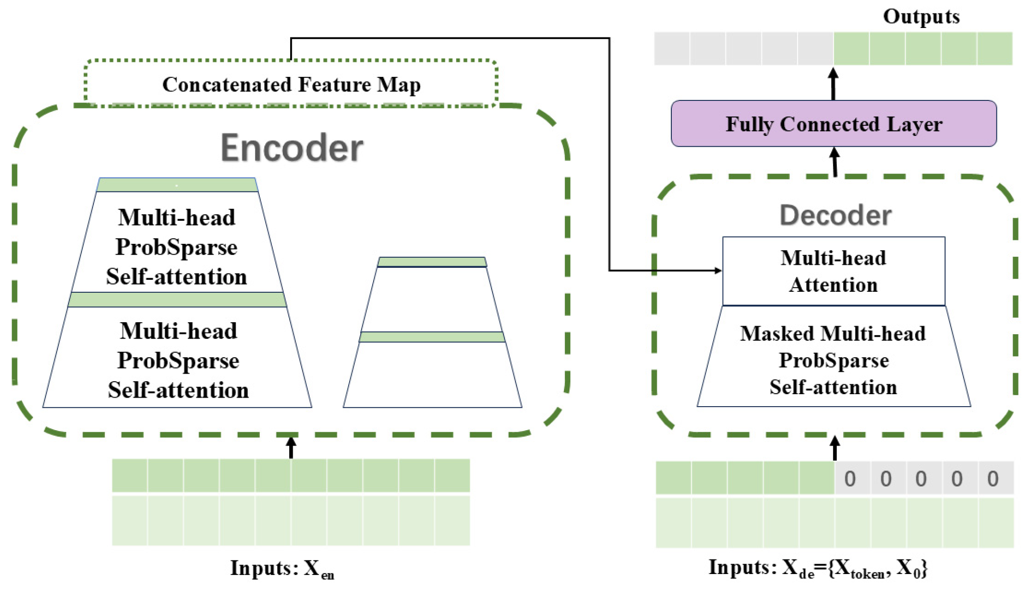
Figure 2 illustrates the structure of the Informer model. The left portion displays the encoder, which consists of stacked modules, each containing a ProbSparse self-attention layer and a distillation layer. The complete input sequence passes through these modules sequentially, with the distillation mechanism progressively reducing the sequence length to lower computational overhead. The output from the final encoder layer is then fed into the decoder.

In most time series, the attention distribution is sparse—only a few key time steps contribute significantly, while most others have negligible weights. To exploit this, Informer introduces the ProbSparse self-attention mechanism, which calculates dot products between each query and only the top-u most relevant keys, followed by softmax normalization. This significantly reduces computational complexity. The computation is given as follows:

$$\mathrm{A}(\mathrm{Q},\mathrm{K},\mathrm{V})=\mathrm{Softmax}\left\{{\displaystyle \frac{{\overline{\mathrm{Q}}\mathrm{K}}^{\mathrm{T}}}{\sqrt{\mathrm{d}}}}\right\}\mathrm{V}$$

(17)

Among them, Q, K, and V represent the input feature matrices. $\overline{\mathrm{Q}}$ is a sparse matrix of the same size as Q, containing only the top-u most significant queries, with all other elements set to zero.

The self-attention distillation mechanism reduces computational complexity and memory usage by refining key information in the feature maps and removing redundant features through convolution, activation, and pooling operations. The distillation process from the j-th layer to the (j+1)-th layer is described as follows:

$${\mathrm{X}}_{\mathrm{j}+1}^{\mathrm{t}}=\mathrm{MaxPool}\left(\mathrm{ELU}\left(\mathrm{Conv}1\mathrm{d}\left({\left[{\mathrm{X}}_{\mathrm{j}}^{\mathrm{t}}\right]}_{\mathrm{AB}}\right)\right)\right)$$

(18)

where [⋅]_AB denotes the attention module. Conv1d performs one-dimensional convolution along the temporal dimension using the ELU activation function and a kernel size of 3. Finally, a max-pooling layer with a stride of 2 is applied to downsample X_t to half of its original length, thereby reducing temporal complexity.

The right portion of Figure 2 presents the Informer decoder, which consists of two multi-head self-attention layers and produces predictions using a generative approach. The input format of the decoder is described as follows:

$${\mathrm{X}}_{\mathrm{de}}^{\mathrm{t}}=\mathrm{Concat}\left({\mathrm{X}}_{\mathrm{token} }^{\mathrm{t}},{\mathrm{X}}_0^{\mathrm{t}}\right)\in {\mathrm{R}}^{\left({\mathrm{L}}_{\mathrm{token} }+{\mathrm{L}}_{\mathrm{y}}\right)\times {\mathrm{d}}_{\mathrm{model} }}$$

(19)

where ${\mathrm{X}}_{\mathrm{token}}^{\mathrm{t}}\in {\mathrm{R}}^{{\mathrm{L}}_{\mathrm{token}}\times {\mathrm{d}}_{\mathrm{model}}}$ is the start token, and ${\mathrm{X}}_0^{\mathrm{t}}{\in \mathrm{R}}^{{\mathrm{L}}_{\mathrm{y}}\times {\mathrm{d}}_{\mathrm{model}}}$ is a placeholder for the target sequence, initialized with zeros.

2.5. The Proposed Method

In practical applications, the capacity of lithium-ion batteries gradually degrades over extended periods of use. However, this process is often accompanied by occasional short-term capacity recoveries. To mitigate the impact of these recovery phenomena on prediction results and address potential overfitting or underfitting that may arise from using a single network, this study proposes a prediction method based on CEEMDAN-DInformer-LSTM.

The original capacity degradation sequence of the lithium battery is decomposed into multiple IMFs and a residual component by using the CEEMDAN algorithm. The IMFs capture local oscillatory features and reflect multi-scale high-frequency and mid-frequency variations. These fluctuations often correspond to short-term capacity recovery events caused by factors such as material degradation, SEI layer growth, and loss of active material. Due to their frequent and sharp oscillations, the IMFs are regarded as high-frequency components. In contrast, the residual represents the low-frequency trend that cannot be further decomposed and primarily reflects the long-term degradation of battery capacity over successive cycles. This component exhibits smooth and consistent behavior and is therefore regarded as the low-frequency component. By separating short-term fluctuations from the long-term trend, the proposed method substantially reduces the adverse impact of capacity recovery phenomena on prediction accuracy.

High-frequency components often exhibit intense and frequent oscillations, which reduce the predictive performance of models. To mitigate this issue, this study adopts the data decomposition strategy proposed in DLinear [30]. In this approach, the highly fluctuating high-frequency features are further decomposed into a trend component and a remainder component to reduce volatility. These components are then input into the Informer network for prediction. Finally, the predicted trend and remainder are integrated to yield the final prediction of the high-frequency component. The decomposition procedure is described as follows:

$$\mathrm{T}\left(\mathrm{t}\right)={\displaystyle \frac{1}{\mathrm{k}}}{\displaystyle \sum _{\mathrm{i}=0}^{\mathrm{k}-1}\mathrm{X}}(\mathrm{t}-\mathrm{i})$$

(20)

$$\mathrm{R}\left(\mathrm{t}\right)=\mathrm{X}\left(\mathrm{t}\right)-\mathrm{T}\left(\mathrm{t}\right)$$

(21)

For the processing of low-frequency components, their smooth variations and strong trend characteristics allow simple models to achieve satisfactory predictive performance. In contrast, employing complex models may result in overfitting to the stable trend, capturing irrelevant minor fluctuations, and thereby degrading predictive accuracy. Additionally, complex models often incur longer training times and higher computational costs, leading to inefficient use of resources. To address this, an LSTM model—well-suited for modeling simple time series—is adopted to forecast the low-frequency components. This method improves prediction accuracy without compromising training efficiency or model generalization.

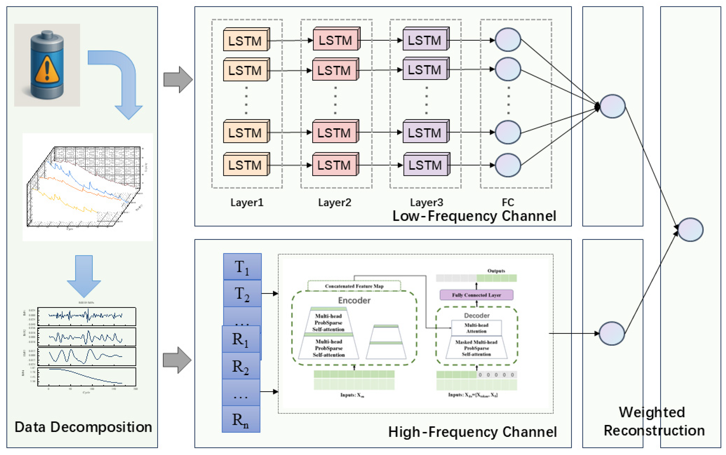
Finally, the predicted outputs of all components are integrated using a weighted reconstruction strategy. As each component carries a different amount of information and contributes unequally to the original signal, directly aggregating their predictions may obscure key patterns with noise or introduce excessive irrelevant fluctuations, impairing the model’s predictive accuracy and stability. To address this issue, the Pearson correlation coefficient is adopted to quantify the importance of each component relative to the original sequence. These correlation-based importance scores then serve as weights during reconstruction, guiding the weighted fusion of component predictions to generate the final output. This approach enhances the utilization of informative signals while suppressing noise, thereby improving the model’s accuracy, robustness, and generalization. The overall model architecture is shown in Figure 3 and the detailed model parameter settings are listed in

Table 1. Parameter settings of the proposed model.

Model	Parameter	Value
	dimension	128
Informer	n_heads	8
	n_encoder	2
	n_decoder	1
	learning_rate	0.001
	drop_out	0.1
LSTM	hidden_size	64
	num_layers	2
	learning_rate	0.001

. All codes are run on Pytorch 1.13.1, Python 3.7.4, and Windows 10 system with an Intel Core i5-7200U CPU.

3. Prediction Procedure and Evaluation Metrics

3.1. Prediction Procedure

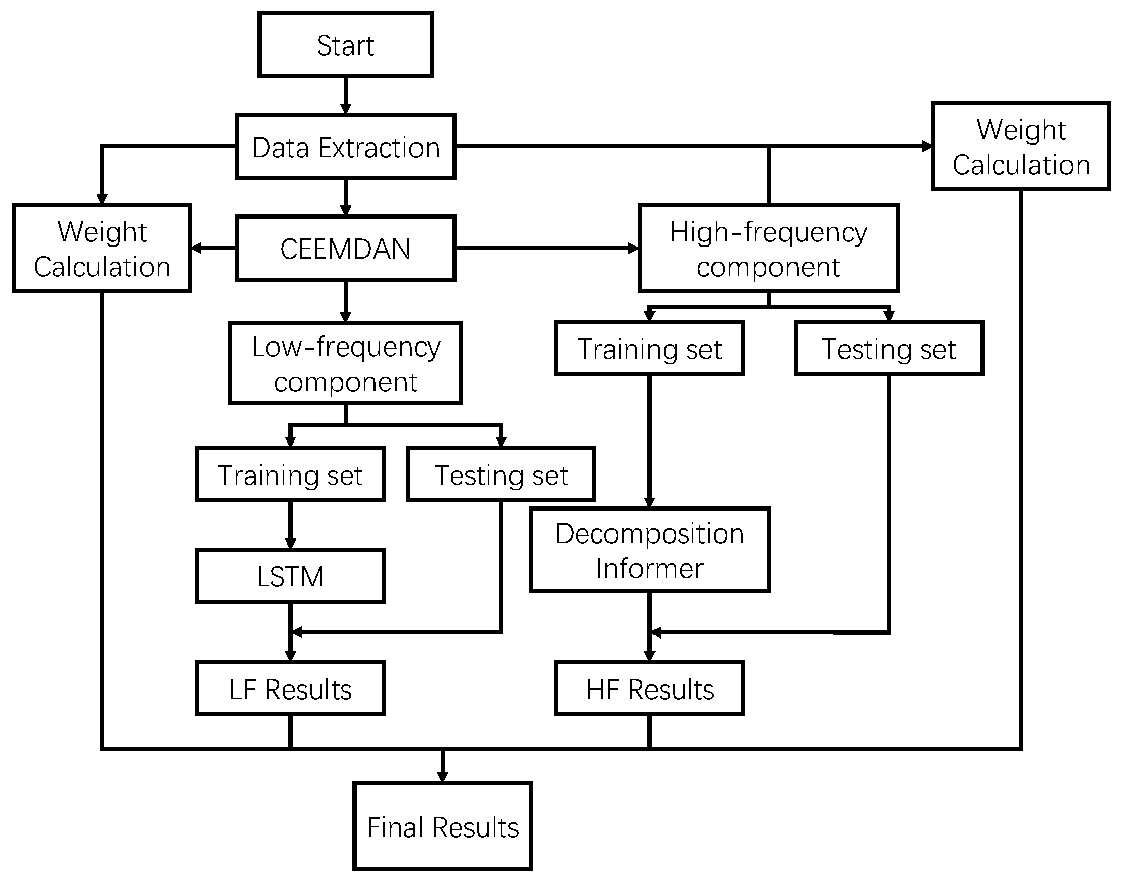
The prediction process of the proposed model is illustrated in Figure 4. The specific steps are as follows:

Step 1: Extract the battery capacity sequences from the dataset. Apply the CEEMDAN algorithm to decompose the capacity data into multiple IMFs.

Step 2: Compute the Pearson correlation coefficient between each IMF and the original capacity sequence. Assign weights to each component based on its correlation value.

Step 3: Further decompose the high-frequency components to capture fine-grained variations. Employ the Informer network to extract latent features and generate corresponding predictions.

Step 4: Use the LSTM model to predict the residual components, leveraging its capability to capture temporal dependencies in time-series data.

Step 5: Perform a weighted summation of the predicted values from all components using the weights obtained in Step 2 to generate the final prediction.

Step 6: Evaluate the model’s performance by comparing the predicted results with the actual capacity data and calculating relevant metrics to assess accuracy, stability, and generalization ability.

3.2. Evaluation Metrics

To evaluate the performance of the proposed model, the following commonly used metrics are employed: mean absolute error (MAE), mean absolute percentage error (MAPE), root-mean-square error (RMSE), R-squared (R²), and RUL_error. Their definitions are provided as follows:

$$\mathrm{MAE}={\displaystyle \frac{1}{\mathrm{n}}}{\displaystyle \sum _{\mathrm{i}=1}^{\mathrm{n}}\left|{\mathrm{y}}_{\mathrm{i}}-{\widehat{\mathrm{y}}}_{\mathrm{i}}\right|}$$

(22)

$$\mathrm{MAPE}={\displaystyle \frac{1}{\mathrm{n}}}{\displaystyle \sum _{\mathrm{i}=1}^{\mathrm{n}}\left|\frac{{\mathrm{y}}_{\mathrm{i}}-{\widehat{\mathrm{y}}}_{\mathrm{i}}}{{\mathrm{y}}_{\mathrm{i}}}\right|}\times 100\%$$

(23)

$$\mathrm{RMSE}=\sqrt{{\displaystyle \frac{1}{\mathrm{n}}}{\displaystyle \sum _{\mathrm{i}=1}^{\mathrm{n}}{\left({\mathrm{y}}_{\mathrm{i}}-{\widehat{\mathrm{y}}}_{\mathrm{i}}\right)}^2}}$$

(24)

$${\mathrm{R}}^2=1-{\displaystyle \frac{{\displaystyle \sum _{\mathrm{i}=1}^{\mathrm{n}}{\left({\mathrm{y}}_{\mathrm{i}}-{\widehat{\mathrm{y}}}_{\mathrm{i}}\right)}^2}}{{\displaystyle \sum _{\mathrm{i}=1}^{\mathrm{n}}{\left({\overline{\mathrm{y}}}_{\mathrm{i}}{-\mathrm{y}}_{\mathrm{i}}\right)}^2}}}$$

(25)

$${\mathrm{RUL}}_{\mathrm{error}}=|{\mathrm{RUL}}_{\mathrm{PRE}}-{\mathrm{RUL}}_{\mathrm{TRUE}}|$$

(26)

where n is the length of the sequence, y_i denotes the actual value, and ${\widehat{\mathrm{y}}}_{\mathrm{i}}$ denotes the predicted value. RUL_PRE denotes the cycle when the predicted capacity falls below the failure threshold, and RUL_TRUE denotes the current cycle at which the actual capacity falls below the failure threshold.

4. Experiments and Results Analysis

4.1. Datasets

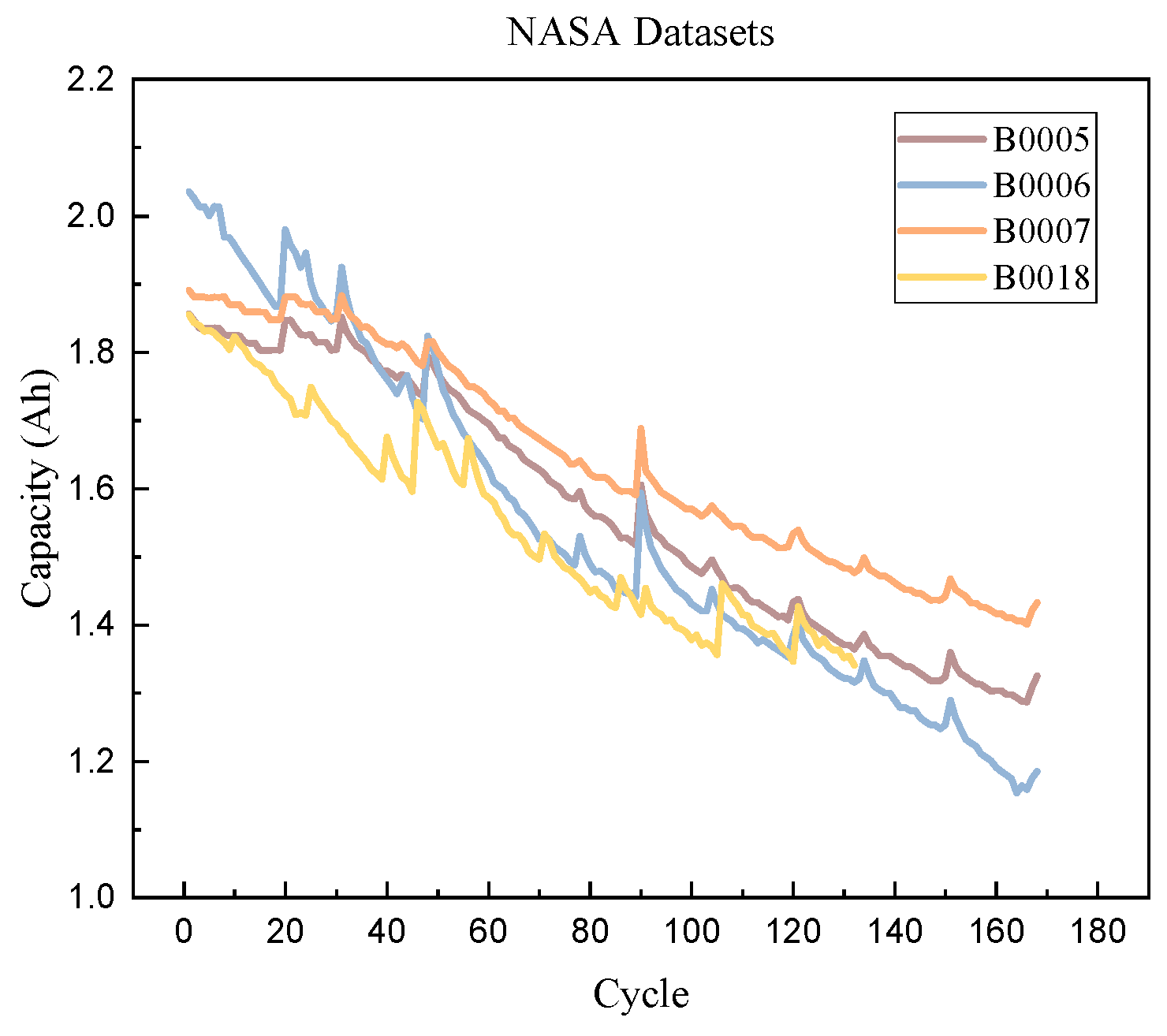
In this study, four battery datasets—B0005, B0006, B0007, and B0018—were selected from the publicly available lithium-ion battery dataset provided by the NASA Ames Research Center [31]. These datasets include charge–discharge profiles and impedance measurements recorded at a room temperature of 24 °C.

During charging, a constant current (CC) of 1.5 A was applied until the voltage reached 4.2 V, followed by constant voltage (CV) charging at 4.2 V until the current dropped to 20 mA. During discharging, a constant current of 2 A was applied until the terminal voltage reached 2.7 V, 2.5 V, 2.2 V, and 2.5 V for B0005, B0006, B0007, and B0018, respectively.

The end-of-life (EOL) of the NASA batteries is defined as the point when the capacity drops to 70% of its initial value (i.e., 1.4 Ah). Since the B0007 battery did not reach EOL at the end of data collection, its EOL was set to 75% of the initial capacity (i.e., 1.5 Ah) for evaluation metric calculation. The capacity degradation curves over the cycle count for the four batteries are illustrated in Figure 5.

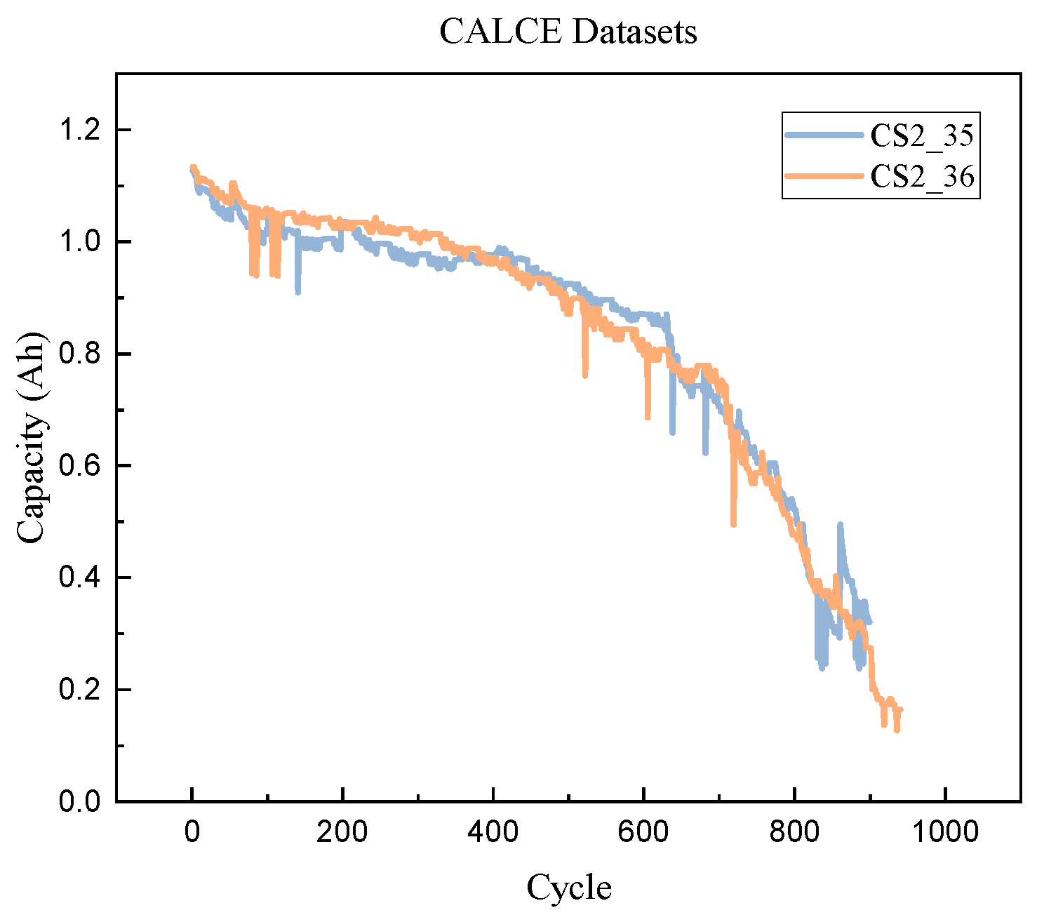
To further evaluate the generalization capability of the proposed model, two additional batteries, CS2_25 and CS2_26, were selected from the lithium-ion battery cycle life dataset provided by the Center for Advanced Life Cycle Engineering (CALCE) at the University of Maryland. In this dataset, the batteries operate at a constant temperature. During charging, a constant current (CC) is applied until the voltage reaches 4.2 V, followed by constant voltage (CV) charging until the current drops to 20 mA. The discharging process is performed in constant current mode until the battery voltage decreases to 2.7 V. The end of battery life is defined as the point when the capacity falls to 70% of its rated capacity (1.1 Ah), i.e., 0.77 Ah. The capacity degradation curves of the two CALCE batteries versus the number of cycles are illustrated in Figure 6.

4.2. CEEMDAN

Taking batteries B0005 and CS2_35 as examples, both exhibited an overall declining trend in capacity over their respective life cycles. However, varying degrees of capacity recovery were also observed during the degradation process. To better capture these fluctuations, the original capacity data were decomposed using CEEMDAN. Figure 7 presents the decomposition results for B0005 and CS2_35.

For battery B0005, the capacity sequence was decomposed into four IMFs. Among them, IMF1 to IMF3 represented high-frequency components characterized by noticeable oscillations, while IMF4 served as the residual component, displaying a smooth and dominant trend. In contrast, the CS2_35 battery was decomposed into seven IMFs, with IMF1 to IMF6 corresponding to high-frequency components and IMF7 representing the overall trend.

4.3. Pearson Correlation Coefficient

The original capacity data were decomposed into several IMFs using the CEEMDAN method, each representing a distinct frequency component of the signal with varying influence on the original data. To enhance prediction accuracy, certain components were selectively emphasized rather than directly summed. Their relevance was quantified by calculating the Pearson correlation coefficient between each IMF and the original capacity sequence, and these coefficients served as weights in a weighted aggregation after model prediction. The weights derived from the NASA dataset are presented in

Table 2. Weighting coefficients of decomposed components.

Battery	IMF1	IMF2	IMF3	IMF4
B0005	0.0623	0.1796	0.1325	1
B0006	0.1325	0.1522	0.1424	1
B0007	0.0747	0.1628	0.0153	1
B0018	0.0731	0.1185	0.4271	1

. Since IMF4 reflects the underlying trend, its weight is fixed at 1, and the weights of the remaining IMFs are scaled proportionally.

4.4. Results and Analysis

To evaluate the effectiveness of the proposed model, experiments were performed on four NASA battery datasets. The first 60% of each sequence was designated as the training set, while the remaining 40% was allocated to the test set. The commonly used sliding window method in time series forecasting was adopted. Each sample consisted of eight consecutive time steps as input, with the subsequent time step serving as the prediction target. Five models were considered in the comparison: LSTM, Informer, CEEMDAN-LSTM, CEEMDAN-DInformer, and the proposed CEEMDAN-DInformer-LSTM model.

Each model was applied to predict the remaining useful life of batteries, and four evaluation metrics were calculated to assess performance. The results are summarized in

Table 3. Evaluation metrics of different models.

Battery	Model	MAE	MAPE	RMSE	R2	RULerror (Cycle)
B0005	LSTM	0.0422	0.0315	0.0482	0.9608	13
	Informer	0.0384	0.0291	0.0442	0.9712	7
	CEEMDAN-LSTM	0.0256	0.0191	0.0304	0.9662	3
	CEEMDAN-DInformer	0.0215	0.0159	0.0261	0.9729	2
	CEEMDAN-DInformer-LSTM	0.0199	0.0148	0.0238	0.9937	0
B0006	LSTM	0.0576	0.0466	0.0684	0.9633	5
	Informer	0.0492	0.0406	0.0629	0.9728	4
	CEEMDAN-LSTM	0.0529	0.0418	0.0595	0.9700	4
	CEEMDAN-DInformer	0.0214	0.0171	0.0275	0.9730	3
	CEEMDAN-DInformer-LSTM	0.0172	0.0136	0.0233	0.9855	1
B0007	LSTM	0.0408	0.0281	0.0468	0.9615	21
	Informer	0.0272	0.0189	0.0341	0.9729	12
	CEEMDAN-LSTM	0.0337	0.0231	0.0379	0.9766	5
	CEEMDAN-DInformer	0.0218	0.0149	0.0246	0.9787	5
	CEEMDAN-DInformer-LSTM	0.0147	0.0101	0.0174	0.9903	2
B0018	LSTM	0.0324	0.0235	0.0352	0.9782	4
	Informer	0.0358	0.0260	0.0398	0.9714	2
	CEEMDAN-LSTM	0.0261	0.0165	0.0310	0.9796	2
	CEEMDAN-DInformer	0.0241	0.0172	0.0283	0.9837	2
	CEEMDAN-DInformer-LSTM	0.0175	0.0125	0.0213	0.9908	1

.

From an overall perspective, the single models, LSTM and Informer, exhibited performance fluctuations across different battery datasets. Due to its superior capability in modeling long-time series, Informer generally outperformed LSTM in most cases. However, the presence of capacity regeneration introduces irregular fluctuations in the data, which reduces the prediction accuracy of both models.

By applying CEEMDAN for signal decomposition, the overall model performance improves significantly compared to the single models. For instance, in the case of battery B0005, CEEMDAN-LSTM achieved substantial gains over LSTM, with marked reductions in MAE and MAPE. The RMSE decreased by approximately 36%, and the R² score also improved.

CEEMDAN-DInformer further outperformed CEEMDAN-LSTM, achieving R² values above 0.97 across all four battery datasets, indicating superior fitting and predictive capability. Nonetheless, models based on a single network structure still suffered from limited feature extraction, restricting further accuracy gains.

In contrast, the proposed CEEMDAN-DInformer-LSTM model achieved the best performance across all evaluation metrics, with the average R² value across different batteries being approximately 0.99—representing a 1–2% improvement. For battery B0007 in particular, the model achieves an MAE of 0.0147, an MAPE of 0.0101, and an R² score of 0.9903, highlighting the hybrid model’s comprehensive advantages in error control, trend fitting, and generalization.

To provide a clearer comparison of predictive performance, Figure 8 shows the prediction results of different models on four batteries from the NASA dataset. As shown in the figure, all models were able to capture the early-stage capacity decline trend. However, as degradation progressed, differences in model performance became more pronounced. Near the failure threshold, the baseline models displayed marked prediction errors and lag, along with fluctuations in the predicted curves. This reflected their limited ability to model the nonlinear characteristics of late-stage degradation, which led to unstable RUL estimates and increased operational risks in real-world applications.

Alternatively, the proposed CEEMDAN-DInformer-LSTM model improved the modeling of complex, non-stationary signals by separately processing high- and low-frequency components and integrating them through weighted fusion. Both quantitative evaluation metrics and the visual fitting results confirmed that this model consistently outperforms the others, thereby improving the reliability and robustness of RUL prediction.

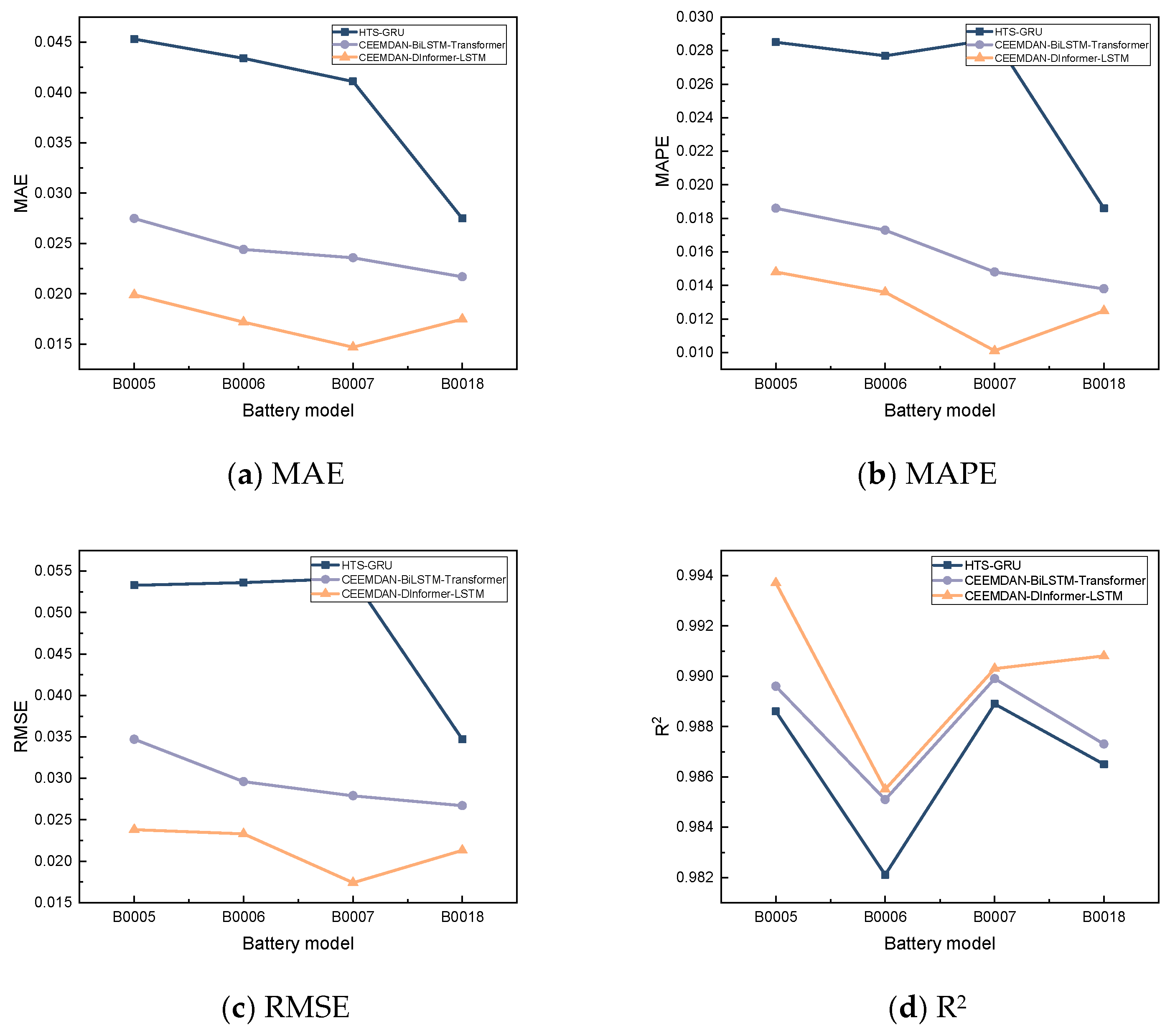
Secondly, to further validate the effectiveness of the proposed model, its experimental results on the NASA dataset were compared with two recently proposed improved models from the past year: HTS-GRU [32] and CEEMDAN-BiLSTM-Transformer [28]. Consistent with the previous experiments, the first 60% of each sequence was used for training, while the remaining 40% was used for testing. The evaluation results are presented in Figure 9.

Among the four battery datasets, the CEEMDAN-DInformer-LSTM model achieved the best results across all evaluation metrics. Compared with the HTS-GRU model, it reduced the MAE by 56.1% and the RMSE by 55.3% on battery B0005. For battery B0007, the RMSE dropped from 0.0541 to 0.0174, representing a 67.8% reduction in error. On battery B0006, compared with the CEEMDAN-BiLSTM-Transformer model, the MAE decreased from 0.0244 to 0.0172, the RMSE decreased from 0.0296 to 0.0233, and the R² increased to 0.9855. Battery B0018 also showed stable performance, with the MAE and RMSE reduced by 19.4% and 20.2%, respectively, while the R² improved from 0.9873 to 0.9908. These results demonstrated that CEEMDAN-DInformer-LSTM consistently achieved high prediction accuracy across different datasets, confirming the effectiveness of the proposed method for lithium-ion battery RUL prediction.

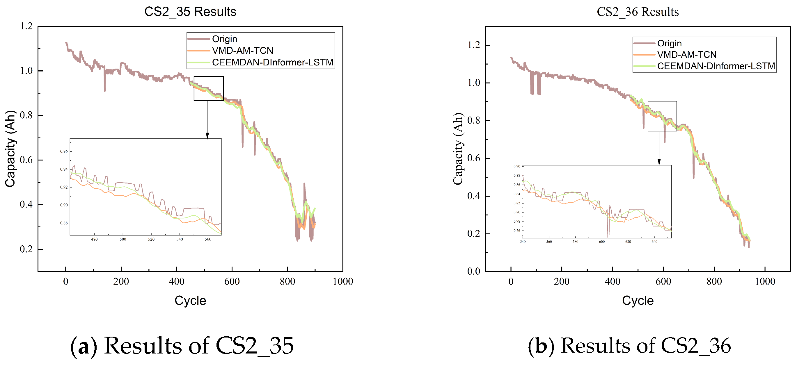
Finally, to validate the generalization capability of the proposed model under varying data conditions, two batteries—CS2_35 and CS2_36—from the CALCE dataset were selected. These batteries differed in type and operating conditions. The first 50% of each sequence was used as the training set and the remaining 50% was used as the test set. To ensure a fair comparison, all experiments were conducted under identical settings, and the performance of the CEEMDAN-DInformer-LSTM model was compared with that of the recently proposed VMD-AM-TCN model [33].

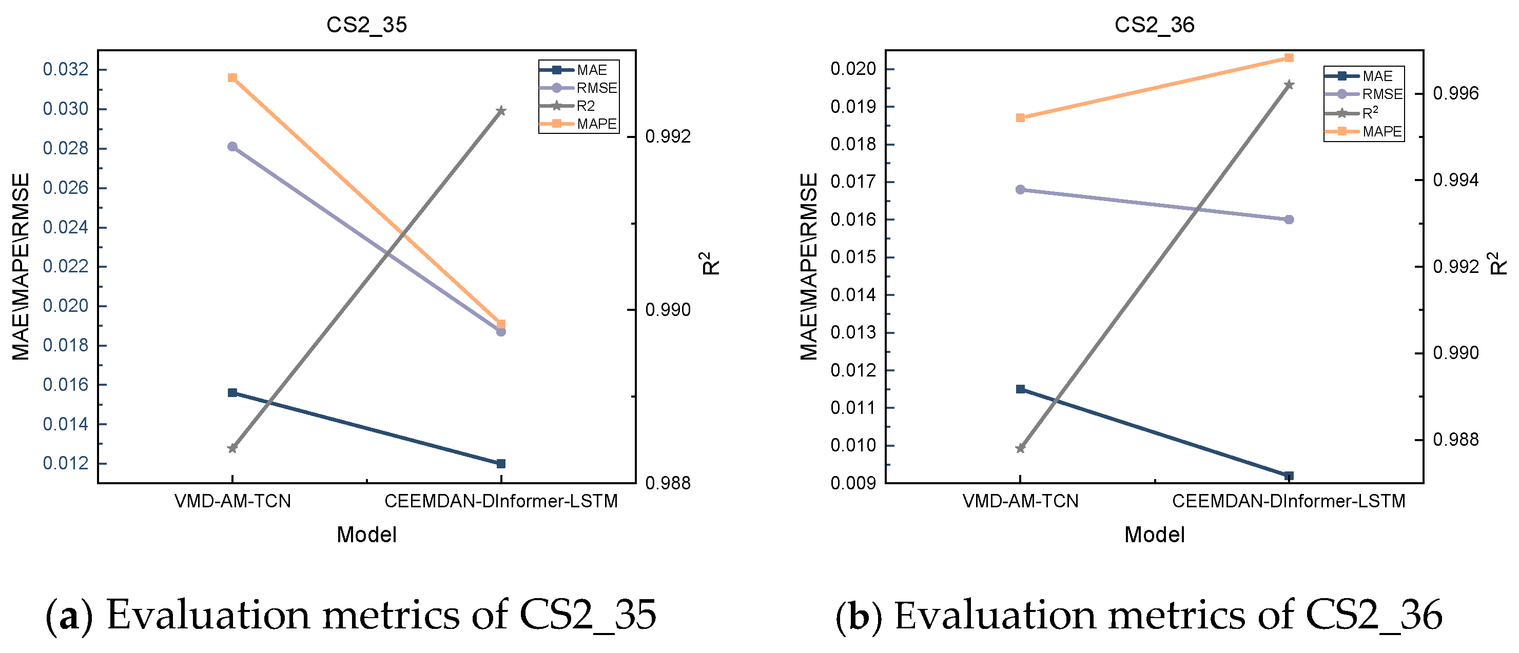
Figure 10 and Figure 11 present the prediction results and evaluation metrics for the two CALCE batteries. As shown in Figure 10, although both prediction methods can effectively fit the actual battery capacity degradation curves, compared to VMD-AM-TCN, CEEMDAN-DInformer-LSTM more accurately predicted short-term high-frequency fluctuations, demonstrating enhanced predictive performance. To provide a more intuitive comparison of the predictive performance of the two methods, Figure 11 presents the specific evaluation metrics for both batteries. For CS2_35, the CEEMDAN-DInformer-LSTM model outperformed VMD-AM-TCN across all evaluation metrics: MAE decreased from 0.0156 to 0.0120, MAPE from 0.0316 to 0.0191, and RMSE from 0.0281 to 0.0187. The R² score improved from 0.9884 to 0.9923, indicating higher prediction accuracy and better curve-fitting performance. For CS2_36, although the proposed model showed a slightly higher MAPE compared to VMD-AM-TCN, it still achieved better overall accuracy, with superior MAE, RMSE, and R² performance.

These results demonstrated that the proposed CEEMDAN-DInformer-LSTM model showed strong and stable predictive performance across different battery types and operating conditions, confirming its robust generalization ability and practical applicability.

5. Conclusions

Reliable prediction of lithium-ion batteries’ RUL is vital for ensuring the safe and stable operation of the equipment. To address the effects of capacity regeneration and the limited feature extraction caused by single-model prediction and improve prediction accuracy, this study proposed a hybrid RUL prediction model for lithium-ion batteries, integrating CEEMDAN signal decomposition, Informer, and LSTM networks. The proposed method was evaluated on four batteries (B0005, B0006, B0007, and B0018) from the NASA dataset, and on two batteries (CS2_35 and CS2_36) from the CALCE dataset.

The experimental results indicated that the proposed CEEMDAN-DInformer-LSTM model significantly outperformed single models in terms of predictive accuracy across all four NASA batteries. Across the four NASA batteries, the proposed method achieved average MAE, MAPE, and RMSE values of approximately 0.0173, 0.0138, and 0.0227. Compared with methods proposed in the past year, it achieved the best performance across all evaluation metrics. On the CALCE dataset, the proposed method also demonstrated better performance, further confirming its enhanced robustness and predictive capability across different battery types and datasets.

References

1. Nourianfar, H.; Abdi, H. Economic emission dispatch considering electric vehicles and wind power using enhanced multi-objective exchange market algorithm. J. Clean. Prod. 2023, 415, 137805. [Google Scholar] [CrossRef]
2. Lipu, M.H.; Abd Rahman, M.; Mansor, M.; Ansari, S.; Meraj, S.T.; Hannan, M. Hybrid and combined states estimation approaches for lithium-ion battery management system: Advancement, challenges and future directions. J. Energy Storage 2024, 92, 112107. [Google Scholar] [CrossRef]
3. Zhao, B.; Zhang, W.; Zhang, Y.; Zhang, C.; Zhang, C.; Zhang, J. Lithium-ion battery remaining useful life prediction based on interpretable deep learning and network parameter optimization. Appl. Energy 2025, 379, 124713. [Google Scholar] [CrossRef]
4. You, H.; Zhu, J.; Wang, X.; Jiang, B.; Wei, X.; Dai, H. Nonlinear aging knee-point prediction for lithium-ion batteries faced with different application scenarios. Etransportation 2023, 18, 100270. [Google Scholar] [CrossRef]
5. Shrivastava, P.; Naidu, P.A.; Sharma, S.; Panigrahi, B.K.; Garg, A. Review on technological advancement of lithium-ion battery states estimation methods for electric vehicle applications. J. Energy Storage 2023, 64, 107159. [Google Scholar] [CrossRef]
6. Zhang, D.; Li, W.; Han, X.; Lu, B.; Zhang, Q.; Bo, C. Evolving Elman neural networks based state-of-health estimation for satellite lithium-ion batteries. J. Energy Storage 2023, 59, 106571. [Google Scholar] [CrossRef]
7. Lyu, G.; Zhang, H.; Zhang, Y.; Miao, Q. An interpretable remaining useful life prediction scheme of lithium-ion battery considering capacity regeneration. Microelectron. Reliab. 2022, 138, 114625. [Google Scholar] [CrossRef]
8. Lyu, G.; Zhang, H.; Miao, Q. Parallel state fusion LSTM-based early-cycle stage lithium-ion battery RUL prediction under Lebesgue sampling framework. Reliab. Eng. Syst. Saf. 2023, 236, 109315. [Google Scholar] [CrossRef]
9. Pang, H.; Chen, K.; Geng, Y.; Wu, L.; Wang, F.; Liu, J. Accurate capacity and remaining useful life prediction of lithium-ion batteries based on improved particle swarm optimization and particle filter. Energy 2024, 293, 130555. [Google Scholar] [CrossRef]
10. Zhang, Y.; Xiong, R.; He, H.; Pecht, M. Validation and verification of a hybrid method for remaining useful life prediction of lithium-ion batteries. J. Clean. Prod. 2019, 212, 240–249. [Google Scholar] [CrossRef]
11. Wang, R.; Zhu, M.; Zhang, X.; Pham, H. Lithium-ion battery remaining useful life prediction using a two-phase degradation model with a dynamic change point. J. Energy Storage 2023, 59, 106457. [Google Scholar] [CrossRef]
12. Ezzouhri, A.; Charouh, Z.; Ghogho, M.; Guennoun, Z. A data-driven-based framework for battery remaining useful life prediction. IEEE Access 2023, 11, 76142–76155. [Google Scholar] [CrossRef]
13. Long, T.; Wang, S.; Cao, W.; Zhou, H.; Fernandez, C. An improved variable forgetting factor recursive least square-double extend Kalman filtering based on global mean particle swarm optimization algorithm for collaborative state of energy and state of health estimation of lithium-ion batteries. Electrochim. Acta 2023, 450, 142270. [Google Scholar] [CrossRef]
14. Tian, Y.; Huang, Z.; Tian, J.; Li, X. State of charge estimation of lithium-ion batteries based on cubature Kalman filters with different matrix decomposition strategies. Energy 2022, 238, 121917. [Google Scholar] [CrossRef]
15. Wu, J.; Meng, J.; Lin, M.; Wang, W.; Wu, J.; Stroe, D.-I. Lithium-ion battery state of health estimation using a hybrid model with electrochemical impedance spectroscopy. Reliab. Eng. Syst. Saf. 2024, 252, 110450. [Google Scholar] [CrossRef]
16. Wang, Y.; Zhang, X.; Liu, K.; Wei, Z.; Hu, X.; Tang, X.; Chen, Z. System identification and state estimation of a reduced-order electrochemical model for lithium-ion batteries. Etransportation 2023, 18, 100295. [Google Scholar] [CrossRef]
17. Park, J.; Jin, Y.; Kam, W.; Han, S. A practical semi-empirical model for predicting the SoH of lithium-ion battery: A novel perspective on short-term rest. J. Energy Storage 2024, 96, 112659. [Google Scholar] [CrossRef]
18. Han, X.; Zhang, J.; Fu, D. Lifetime prediction of power electrolytic capacitors based on IKH-UKF-PF. J. Power Supply 2024, 1–12. [Google Scholar]
19. Wang, S.; Ma, H.; Zhang, Y.; Li, S.; He, W. Remaining useful life prediction method of lithium-ion batteries is based on variational modal decomposition and deep learning integrated approach. Energy 2023, 282, 128984. [Google Scholar] [CrossRef]
20. Wei, R.; Mao, T.; Gao, H.; Peng, J.; Yang, J. Health state estimation of lithium ion battery based on TWP-SVR. Energy Storage Sci. Technol. 2022, 11, 2585. [Google Scholar]
21. JIN, H.; HU, Y.; GE, H.; HAO, Z.; ZENG, Z.; TANG, Z. Remaining useful life prediction for lithium-ion batteries based on an improved GWO–SVR algorithm. Chin. J. Eng. 2024, 46, 514–524. [Google Scholar]
22. Feng, J.; Cai, F.; Li, H.; Huang, K.; Yin, H. A data-driven prediction model for the remaining useful life prediction of lithium-ion batteries. Process Saf. Environ. Prot. 2023, 180, 601–615. [Google Scholar] [CrossRef]
23. Jia, Z.; Li, Z.; Zhao, K.; Wang, K.; Wang, S.; Liu, Z. CNN-DBLSTM: A long-term remaining life prediction framework for lithium-ion battery with small number of samples. J. Energy Storage 2024, 97, 112947. [Google Scholar] [CrossRef]
24. Vaswani, A.; Shazeer, N.; Parmar, N.; Uszkoreit, J.; Jones, L.; Gomez, A.N.; Kaiser, Ł.; Polosukhin, I. Attention is all you need. arXiv 2017, arXiv:1706.03762. [Google Scholar] [PubMed]
25. Chen, D.; Hong, W.; Zhou, X. Transformer network for remaining useful life prediction of lithium-ion batteries. IEEE Access 2022, 10, 19621–19628. [Google Scholar] [CrossRef]
26. Meng, J.; Azib, T.; Yue, M. Early-Stage end-of-Life prediction of lithium-Ion battery using empirical mode decomposition and particle filter. Proc. Inst. Mech. Eng. Part A J. Power Energy 2023, 237, 1090–1099. [Google Scholar] [CrossRef]
27. Torres, M.E.; Colominas, M.A.; Schlotthauer, G.; Flandrin, P. A complete ensemble empirical mode decomposition with adaptive noise. In Proceedings of the 2011 IEEE International Conference on Acoustics, Speech and Signal Processing (ICASSP), Prague, Czech Republic, 22–27 May 2011; IEEE: New York, NY, USA, 2011; pp. 4144–4147. [Google Scholar]
28. Liu, B.; Ji, C.; Cao, L.; Wu, X.; Duan, Y. Prediction of Remaining Service Life of Lithium-Ion Batteries Based on Complete Ensemble Empirical Mode Decomposition with Adaptive Noise and BiLSTM-Transformer. Power Syst. Prot. Control 2024, 52, 167–177. [Google Scholar]
29. Zhou, H.; Zhang, S.; Peng, J.; Zhang, S.; Li, J.; Xiong, H.; Zhang, W. Informer: Beyond efficient transformer for long sequence time-series forecasting. In Proceedings of the AAAI Conference on Artificial Intelligence, Virtual, 2–9 February 2021; pp. 11106–11115. [Google Scholar]
30. Zeng, A.; Chen, M.; Zhang, L.; Xu, Q. Are transformers effective for time series forecasting? In Proceedings of the AAAI conference on artificial intelligence, Washington, DC, USA, 7–14 February 2023; pp. 11121–11128. [Google Scholar]
31. Saha, B.; Goebel, K. Battery data set. In NASA AMES Prognostics Data Repository; NASA: Washington, DC, USA, 2007. [Google Scholar]
32. Lin, D.; Zhang, J. Lithium-ion battery life prediction based on improved HTS-GRU. J. Power Supply 2024, 1–14. [Google Scholar]
33. Wang, G.; Sun, L.; Wang, A.; Jiao, J.; Xie, J. Lithium battery remaining useful life prediction using VMD fusion with attention mechanism and TCN. J. Energy Storage 2024, 93, 112330. [Google Scholar] [CrossRef]
Figure 1. LSTM cell structure diagram.
Electronics 14 03886 g001
Figure 2. Informer model structure.
Electronics 14 03886 g002
Figure 3. Diagram of the proposed model.
Electronics 14 03886 g003
Figure 4. Framework of the proposed model.
Electronics 14 03886 g004
Figure 5. NASA battery dataset capacity degradation curve.
Electronics 14 03886 g005
Figure 6. CALCE battery dataset capacity degradation curve.
Electronics 14 03886 g006
Figure 7. IMFs of B0005 and CS2_35 after decomposition.
Electronics 14 03886 g007
Figure 8. Prediction results of five models.
Electronics 14 03886 g008
Figure 9. Line charts of the evaluation metrics on the NASA dataset.
Electronics 14 03886 g009
Figure 10. Comparison of prediction results for CS2_35 and CS2_36.
Electronics 14 03886 g010
Figure 11. Line charts of the evaluation metrics on the CALCE dataset.
Electronics 14 03886 g011