Optimizing Robotic Disassembly-Assembly Line Balancing with Directional Switching Time via an Improved Q(λ) Algorithm in IoT-Enabled Smart Manufacturing

Abstract

With the growing adoption of circular economy principles in manufacturing, efficient disassembly and reassembly of end-of-life (EOL) products has become a key challenge in smart factories. This paper addresses the Disassembly and Assembly Line Balancing Problem (DALBP), which involves scheduling robotic tasks across workstations while minimizing total operation time and accounting for directional switching time between disassembly and assembly phases. To solve this problem, we propose an improved reinforcement learning algorithm, IQ($\lambda$), which extends the classical Q($\lambda$) method by incorporating eligibility trace decay, a dynamic Action Table mechanism to handle non-conflicting parallel tasks, and switching-aware reward shaping to penalize inefficient task transitions. Compared with standard Q($\lambda$), these modifications enhance the algorithm’s global search capability, accelerate convergence, and improve solution quality in complex DALBP scenarios. While the current implementation does not deploy live IoT infrastructure, the architecture is modular and designed to support future extensions involving edge-cloud coordination, trust-aware optimization, and privacy-preserving learning in Industrial Internet of Things (IIoT) environments. Four real-world disassembly-assembly cases (flashlight, copier, battery, and hammer drill) are used to evaluate the algorithm’s effectiveness. Experimental results show that IQ($\lambda$) consistently outperforms traditional Q-learning, Q($\lambda$), and Sarsa in terms of solution quality, convergence speed, and robustness. Furthermore, ablation studies and sensitivity analysis confirm the importance of the algorithm’s core design components. This work provides a scalable and extensible framework for intelligent scheduling in cyber-physical manufacturing systems and lays a foundation for future integration with secure, IoT-connected environments.

1. Introduction

With the rapid evolution of modern manufacturing toward green, intelligent, and connected paradigms, efficient end-of-life (EOL) product disassembly [1,2,3] and resource recovery utilization have emerged as critical enablers of sustainable circular economies. Smart factories, envisioned under the Industrial Internet of Things (IIoT) paradigm [4], aim to integrate autonomous robotic systems, distributed sensing, and secure data infrastructure to enable real-time adaptive disassembly and reassembly operations. While this work does not yet implement IoT infrastructure directly, the proposed modular scheduling framework is explicitly designed to support future integration with IoT-enabled cyber-physical environments [5,6].

Traditional disassembly line balancing problems (DLBP) primarily focus on maximizing the efficiency of disassembly processes for subassembly recovery [7], often neglecting the reassembly or remanufacturing stages that are essential for closed-loop production. To address this limitation, a more comprehensive model, the disassembly and assembly line, has emerged, offering improved resource reutilization and enabling intelligent production with minimal waste [8,9]. Within such systems, the coordination of robotic operations is not only a logistical challenge but also a potential cybersecurity consideration in connected environments, where idle switching times and predictable task sequences may expose the system to timing-based vulnerabilities.

This motivates the study of the disassembly and assembly line balancing problem (DALBP), which demands holistic modeling and optimization of integrated operations [10]. DALBP accounts for the sequencing and allocation of tasks across multiple robotic workstations [11], including the directional switching time required when robots alternate between disassembly and assembly tasks. For example, in an automotive electronics remanufacturing setting, a robot may be required to disassemble an engine control unit and then immediately assemble a reusable circuit board into a new module. Physical reorientation between spatially separated task zones can introduce non-negligible delays. When accumulated over hundreds of cycles, these delays reduce throughput and increase energy consumption. Studies have also shown that ignoring switching time leads to suboptimal scheduling and operational bottlenecks [12,13].

Existing research has explored related areas in disassembly or assembly line optimization. Qin et al. [14] considered human factors in assembly line balancing, while Yang et al. [15] proposed a salp swarm algorithm for robotic disassembly lines. Yin et al. [16] introduced a heuristic approach for multi-product, human–robot disassembly collaboration, and Mete et al. [17] studied parallel DALBP using ant colony optimization. However, these efforts either treated disassembly and assembly in isolation or did not account for robot switching dynamics and potential integration with cyber-physical systems. Moreover, the intersection of task scheduling, reinforcement learning, and system-level resilience in IoT-connected factories remains underexplored.

To address these challenges, this paper presents a modular and extendable scheduling framework for DALBP that supports future integration with IoT-enabled architectures. Our contributions include:

• Proposing an integrated disassembly-assembly line model that explicitly incorporates robotic directional switching time, formulated as a mixed-integer programming (MIP) model to improve practical realism in smart manufacturing contexts.
• Designing an improved reinforcement learning algorithm, IQ($\lambda$), which enhances the classic Q($\lambda$) method via eligibility trace decay, structured state–action mappings, and a novel Action Table (AT) that enables flexible task reuse and efficient decision-making.
• Validating the approach through extensive experiments on four real-world product instances and comparing its performance against Q-learning, Sarsa, standard Q($\lambda$), and the CPLEX solver. The proposed method achieves superior optimization quality and convergence performance, with strong potential for extension into secure, distributed, and adaptive environments.

Although this work does not yet deploy IoT-based data or federated learning mechanisms, it establishes a robust algorithmic and architectural foundation for their integration. The proposed IQ($\lambda$)-based DALBP framework can be readily extended to incorporate edge intelligence, privacy-aware scheduling, and secure communication protocols, which are essential for future IIoT implementations.

The remainder of this paper is organized as follows. Section 2 and Section 3 introduce the problem statement and mathematical formulation. Section 4 presents the improved IQ($\lambda$) algorithm and its enhancements. Section 5 describes the experimental setup and comparative results. Section 6 discusses the broader implications for the development of secure and IoT-ready disassembly systems, and Section 7 concludes the paper with a summary and future research directions.

2. Problem Description

2.1. Problem Statement

The disassembly-assembly line balancing problem (DALBP) addressed in this study is situated in the context of fully robotic smart manufacturing systems [18]. Motivated by the high-risk nature of handling end-of-life (EOL) electronic products and the growing demand for resource-efficient production, the DALBP focuses on the coordinated scheduling of robotic disassembly and assembly tasks across shared workstations. The core objective is to optimize task allocation and sequencing while minimizing directional switching delays and processing time.

While the current implementation does not yet incorporate IoT infrastructure, the proposed system is explicitly designed to support future extensions involving cyber-physical integration. This includes IoT-enabled sensing, edge/cloud control systems, secure communication protocols, and adaptive decision-making under real-time constraints.

Each disassembly task (d-task) involves removing a specific part or subassembly from an EOL product, while each assembly task (a-task) involves reusing selected components to build a new product. Robots autonomously execute these tasks, subject to limitations in tool compatibility, physical positioning, and potential future constraints imposed by wireless communication and sensor feedback.

The physical layout consists of parallel disassembly and assembly lines connected by conveyors and shared robot workstations. Figure 1 illustrates this configuration using an automotive battery example [19]. Disassembly tasks on the upper line selectively extract reusable components (e.g., $1\to 3\to 5\to 7\to 9\to 6$), while assembly tasks on the lower line rebuild new modules using a different task order (e.g., $1\to 3\to 2\to 4\to 5$). In shared workstations (dashed boxes), robots switch between task modes, and the model incorporates switching time due to tool changes or orientation shifts.

Although IoT technologies such as RFID-tracked bins, proximity sensors, and edge controllers are not implemented in this study, the system architecture supports their future integration. Such additions would allow real-time status monitoring, traceability, and secure task dispatch, making the DALBP framework suitable for deployment in cyber-physical production environments [20].

2.2. AND/OR Graphs

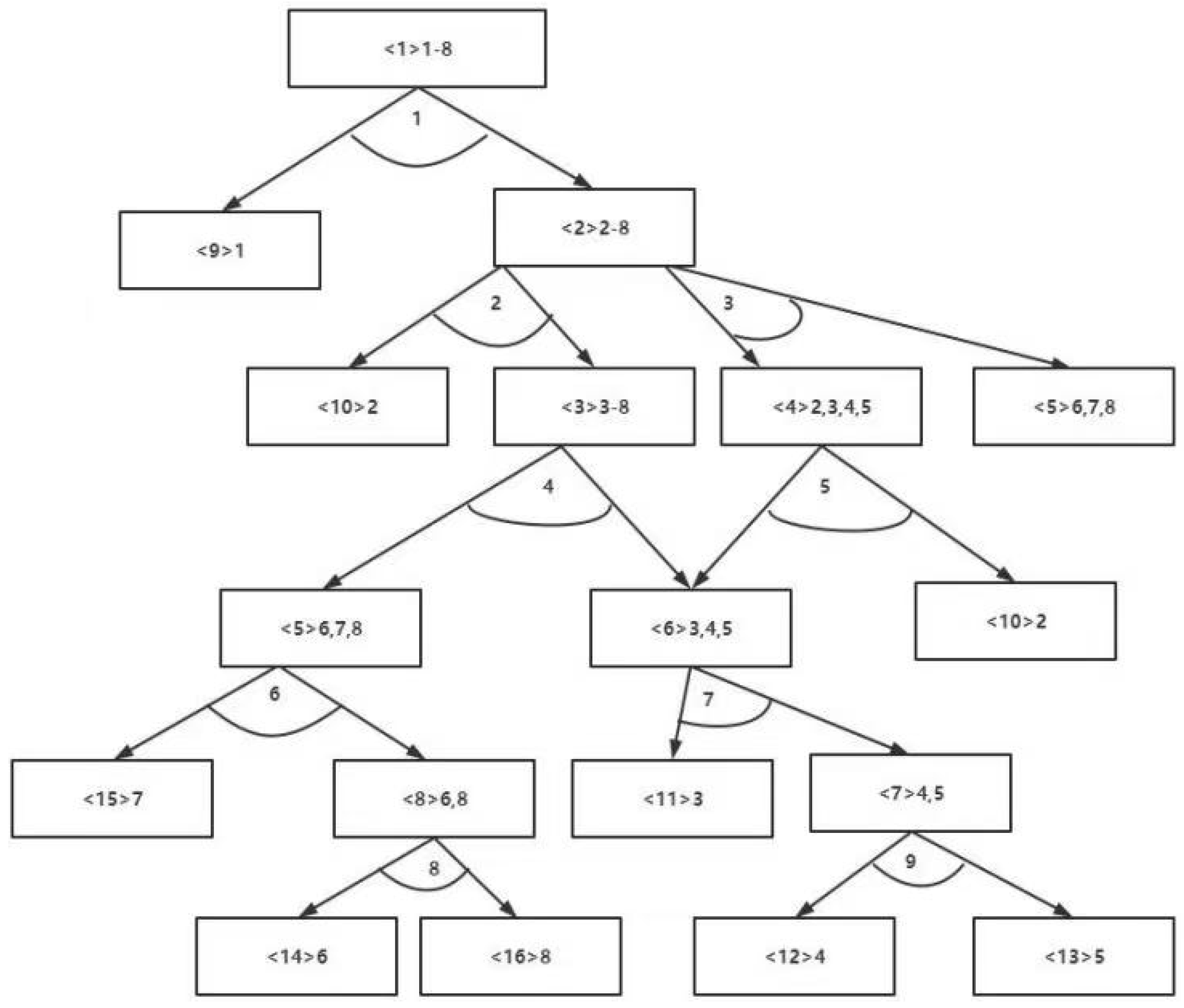
To describe the structure and sequence of disassembly operations, this work employs AND-OR graphs, which model logical dependencies between subassemblies and tasks. These graphs are particularly suitable for representing complex hierarchical relationships in products such as automotive batteries, where components can be removed or reassembled in different configurations depending on product variation or wear level.

AND/OR graphs are digitized into the robotic controller and updated through edge devices, enabling adaptive decision-making based on real-time sensing feedback. In the graph, rectangles represent subassemblies [21,22,23], each containing a unique ID and list of parts. Directed arrows define feasible disassembly transitions. When a subassembly has multiple successors, only one task path is selected at runtime based on heuristic or learned policies.

Figure 2 shows the structural diagram of the product to be disassembled—an automotive battery. Figure 3 presents the corresponding AND/OR graph of the product. In this work, the AND/OR graph is used to represent the disassembly structure of the product. For example, subassembly <1> can be disassembled into subassemblies <2> and <9> through task 1, indicating an AND relationship between subassemblies <2> and <9>. Subassembly <2> can then be disassembled by either task 2 or task 3, representing an OR relationship between tasks 2 and 3.

2.3. Matrix Description

To formally encode precedence and compatibility constraints in the DALBP, matrix-based representations are adopted. These matrices form the input to the optimization model and the state representations for reinforcement learning policies.

• Precedence matrix $S=\left[S_{jk}\right]$ is used to define the relationship between two tasks, where j and k denote IoT-updated disassembly tasks.

  $$S_{jk}=\left\{\begin{array}{cc}1,\hfill & \mathrm{if}\mathrm{task}j\mathrm{must}\mathrm{be}\mathrm{performed}\mathrm{before}\mathrm{task}k\hfill \\ -1,\hfill & \mathrm{if}\mathrm{task}j\mathrm{and}\mathrm{task}k\mathrm{disassemble}\mathrm{the}\mathrm{same}\hfill \\ & \mathrm{assembly}\mathrm{into}\mathrm{different}\mathrm{subassemblies}\hfill \\ 0,\hfill & \mathrm{if}\mathrm{there}\mathrm{is}\mathrm{no}\mathrm{direct}\mathrm{relationship}\mathrm{between}j\hfill \\ & \mathrm{tasks}\mathrm{and}k\hfill \end{array}\right.$$
  Based on the aforementioned description and the AND/OR graph of the automotive battery, the corresponding conflict precedence matrix is obtained as follows:

  $$S=\left[\begin{array}{ccccccccc}0& 1& 1& 1& 1& 1& 1& 1& 1\\ 0& 0& -1& 1& -1& 1& 1& 1& 1\\ 0& -1& 0& -1& 1& 1& 1& 1& 1\\ 0& 0& -1& 0& -1& 1& 1& 1& 1\\ 0& -1& 0& -1& 0& 1& 1& 1& 1\\ 0& 0& 0& 0& 0& 0& 1& 1& 1\\ 0& 0& 0& 0& 0& 0& 0& 1& 1\\ 0& 0& 0& 0& 0& 0& 0& 0& 1\\ 0& 0& 0& 0& 0& 0& 0& 0& 0\end{array}\right]$$
• Task-subassembly relationship matrix $D=\left[d_{ij}\right]$, where $d_{ij}$ represents the relationship between subassembly i and task j, defined as follows. These relationships are also tracked via IoT-based sensors (e.g., RFID tags, smart vision) to verify component flow consistency across lines.

  $$d_{ij}=\left\{\begin{array}{cc}1,\hfill & \mathrm{if}\mathrm{subassembly}i\mathrm{is}\mathrm{generated}\mathrm{by}\mathrm{task}j\hfill \\ -1,\hfill & \mathrm{if}\mathrm{task}j\mathrm{disassembles}\mathrm{subassembly}i\hfill \\ 0,\hfill & \mathrm{otherwise}\hfill \end{array}\right.$$
  Based on the AND/OR diagram of the automotive battery, the task and subassembly relationship matrix can be obtained as follows:

  $$D=\left[\begin{array}{ccccccccc}-1& 0& 0& 0& 0& 0& 0& 0& 0\\ 1& -1& -1& 0& 0& 0& 0& 0& 0\\ 0& 1& 0& -1& 0& 0& 0& 0& 0\\ 0& 0& 1& 0& -1& 0& 0& 0& 0\\ 0& 0& 1& 1& 0& -1& 0& 0& 0\\ 0& 0& 0& 1& 1& 0& -1& 0& 0\\ 0& 0& 0& 0& 0& 0& 1& 0& -1\\ 0& 0& 0& 0& 0& 1& 0& -1& 0\\ 1& 0& 0& 0& 0& 0& 0& 0& 0\\ 0& 1& 0& 0& 1& 0& 0& 0& 0\\ 0& 0& 0& 0& 0& 0& 1& 0& 0\\ 0& 0& 0& 0& 0& 0& 0& 0& 1\\ 0& 0& 0& 0& 0& 0& 0& 0& 1\\ 0& 0& 0& 0& 0& 0& 0& 1& 0\\ 0& 0& 0& 0& 0& 1& 0& 0& 0\\ 0& 0& 0& 0& 0& 0& 0& 1& 0\end{array}\right]$$
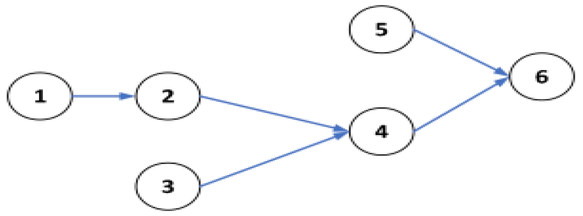
• During the assembly process, assembly tasks must satisfy precedence constraints. These constraints are typically enforced by IoT controllers that validate logic sequences and inter-task timing before dispatching robotic instructions. In this work, the precedence relationships are represented by the matrix $S^a=\left[S_{ik}^a\right]$, which is defined as follows:

  $$S_{ik}^a=\left\{\begin{array}{cc}1,\hfill & \mathrm{if} \mathrm{assembly} \mathrm{task} k \mathrm{is} \mathrm{the} \mathrm{immediate} \mathrm{successor}\hfill \\ \hfill & \mathrm{of} \mathrm{task} i.\hfill \\ 0,\hfill & \mathrm{otherwise}\hfill \end{array}\right.$$
  Suppose that the assembly task priority graph for a certain product is shown in Figure 4. Its assembly priority matrix can be represented as follows:

  $$S^a=\left[\begin{array}{cccccc}0& 1& 0& 0& 0& 0\\ 0& 0& 0& 1& 0& 0\\ 0& 0& 0& 1& 0& 0\\ 0& 0& 0& 0& 0& 1\\ 0& 0& 0& 0& 0& 1\\ 0& 0& 0& 0& 0& 0\end{array}\right]$$

3. Mathematical Model

3.1. Model Assumptions

To facilitate the construction of a linear optimization model tailored for IoT-enabled robotic disassembly-assembly lines, the following assumptions are made:

(1) Task Duration and Profit: The execution time of each disassembly and assembly task is known in advance. Profits from each reusable subassembly are predefined, based on IoT-tracked part value and EOL quality data.

(2) Switching Time: Directional switching times between adjacent tasks are measured in real-time through sensor data and robot telemetry. These delays include repositioning, retooling, and network latency penalties from control signal transmission.

(3) Assembly Sequence: The assembly process begins only after disassembly is completed. IoT-based quality checks and integrity verification are performed before initiating downstream operations.

(4) Cyber-Physical Synchronization: Although currently operating offline, the model is intended to be supervised by edge controllers interfacing with a central planner. Latency, synchronization drift, and network effects are assumed negligible here but will be explored in future real-time deployments.

3.2. Notations

$i$	Index of assembly tasks
$j$	Index of disassembly tasks
$w$	Index of workstations
$e$	Index of subassemblies
$C$	Cycle time for each workstation
$t_d$	Total disassembly time for the product
$t_a$	Total assembly time for the product
${\mathbb{I}}_i^a$	Set of conflicting tasks with assembly task i
${\mathbb{I}}_j^d$	Set of conflicting tasks with disassembly task j
$\mathbb{I}$	Set of all assembly tasks, $\{1,2,\dots ,I\}$
$\mathbb{J}$	Set of all disassembly tasks, $\{1,2,\dots ,J\}$
$\mathbb{E}$	Set of all subassemblies, $\{1,2,\dots ,E\}$
$\mathbb{W}$	Set of all workstations, $\{1,2,\dots ,W\}$
$T_i^a$	Time to perform assembly task i
$T_j^d$	Time to perform disassembly task j
$A_e$	Subassembly node in AND/OR graph
$B_j$	Disassembly task node in AND/OR graph
$P\left(A_e\right)$	Set of immediate predecessors of $A_e$
$S\left(A_e\right)$	Set of immediate successors of $A_e$
${\Gamma }_e$	Disassembly tasks that can produce subassembly e
$ST$	Similar task pairs (assembly and disassembly)
$G_{j{j}^{\prime }}^d$	Directional switching time between disassembly tasks j and $j^{\prime }$
$G_{i{i}^{\prime }}^a$	Directional switching time between assembly tasks i and $i^{\prime }$
$C_i^a$	Unit time cost of performing assembly task i
$C_j^d$	Unit time cost of performing disassembly task j
$C_w$	Operating cost of workstation w
$C_p$	Penalty cost for ungrouped similar tasks
$P_a$	Assembly profit
$P_m$	Maximum possible profit
$R_j$	Profit from disassembling task j

3.3. Decision Variables

$$\begin{array}{cc}\hfill z_w& =\left\{\begin{array}{cc}1,\hfill & \mathrm{if}\mathrm{workstation}w\mathrm{is}\mathrm{opened}\hfill \\ 0,\hfill & \mathrm{otherwise}\hfill \end{array}\right.\hfill \\ \hfill d_{jw}& =\left\{\begin{array}{cc}1,\hfill & \mathrm{if}\mathrm{disassembly}\mathrm{task}j\mathrm{is}\mathrm{assigned}\mathrm{to}\mathrm{workstation}w\hfill \\ 0,\hfill & \mathrm{otherwise}\hfill \end{array}\right.\hfill \\ \hfill a_{iw}& =\left\{\begin{array}{cc}1,\hfill & \mathrm{if}\mathrm{assembly}\mathrm{task}i\mathrm{is}\mathrm{assigned}\mathrm{to}\mathrm{workstation}w\hfill \\ 0,\hfill & \mathrm{otherwise}\hfill \end{array}\right.\hfill \\ \hfill C_j^i& =\left\{\begin{array}{cc}1,\hfill & \mathrm{if}\mathrm{disassembly}\mathrm{task}j\mathrm{is}\mathrm{not}\mathrm{assigned}\mathrm{to}\mathrm{the}\mathrm{same}\hfill \\ \hfill & \mathrm{workstation}\mathrm{as}\mathrm{similar}\mathrm{assembly}\mathrm{task}i\hfill \\ 0,\hfill & \mathrm{otherwise}\hfill \end{array}\right.\hfill \end{array}$$

3.4. Objective Function

$$min(f=t_a+t_d)$$

(1)

3.5. Subject to

$$\sum _{w\in W}{d}_{jw}=1,\forall j\in \mathbb{J}$$

(2)

$$\sum _{w\in W}{a}_{iw}=1,\forall i\in \mathbb{I}$$

(3)

$$\sum _{j\in {\Gamma }_e}\sum _{w\in W}{d}_{jw}=1,\forall e\in \mathbb{E}$$

(4)

$$\sum _{j\in S\left(A_e\right)}\sum _{w\in W}{d}_{jw}\le \sum _{j\in P\left(A_e\right)}\sum _{w\in W}{d}_{jw},\forall e\in \mathbb{E}$$

(5)

$$\sum _i{T}_i^a{a}_{iw}+\sum _j{T}_j^d{d}_{jw}\le C·z_w,\forall w\in \mathbb{W}$$

(6)

$$\begin{array}{cc}\hfill \sum _{j\in \mathbb{J}}{R}_j+P_a& -\sum _{j\in \mathbb{J}}{T}_j^d{C}_j^d+\sum _{i\in \mathbb{I}}{T}_i^a{C}_i^a+\sum _{w\in \mathbb{W}}{C}_w{z}_w\hfill \\ \hfill & +\sum _{(i,j)\in ST}{C}_p{C}_j^i\ge P_m\hfill \end{array}$$

(7)

$$\sum _{w^{\prime }=1}^w\sum _{B_j\in P\left(A_e\right)}{d}_{j{w}^{\prime }}\ge \sum _{B_j\in S\left(A_e\right)}{d}_{jw},\forall e\in \mathbb{E},\forall w\in \mathbb{W}$$

(8)

$$\sum _{w\in \mathbb{W}}w{a}_{iw}\ge \sum _{w\in \mathbb{W}}w{a}_{kw},\forall (i,k)\in S^a$$

(9)

$$t_d\ge \sum _{j,w}{T}_j^d{d}_{jw}+\sum _{j,j^{\prime },w}{G}_{j{j}^{\prime }}^d{d}_{jw}{d}_{j^{\prime }w}$$

(10)

$$t_a\ge \sum _{i,w}{T}_i^a{a}_{iw}+\sum _{i,i^{\prime },w}{G}_{i{i}^{\prime }}^a{a}_{iw}{a}_{i^{\prime }w}$$

(11)

$$d_{jw}+d_{j^{\prime }w}\le 1,\forall (j,j^{\prime })\in {\mathbb{I}}_j^d,\forall w\in \mathbb{W}$$

(12)

$$a_{iw}+a_{i^{\prime }w}\le 1,\forall (i,i^{\prime })\in {\mathbb{I}}_i^a,\forall w\in \mathbb{W}$$

(13)

$$C_j^i\ge a_{iw}-d_{jw},\forall (i,j)\in ST,\forall w\in \mathbb{W}$$

(14)

$$C_j^i\ge d_{jw}-a_{iw},\forall (i,j)\in ST,\forall w\in \mathbb{W}$$

(15)

$$d_{jw},a_{iw},C_j^i,z_w\in \{0,1\},\forall j,i,w$$

(16)

Objective function (Equation (1)): Minimizes total disassembly and assembly time. Constraint (2) ensures each disassembly task must be assigned to exactly one workstation; Constraint (3) ensures each assembly task must be assigned to exactly one workstation; Constraint (4) ensures each subassembly must be generated by exactly one disassembly task; Constraint (5) ensures the number of executed successor tasks for a subassembly cannot exceed that of its predecessor tasks; Constraint (6) ensures total operation time per workstation must not exceed cycle time; Constraint (7) ensures total profit must meet the minimum threshold; Constraint (8) ensures predecessor tasks of a subassembly must be completed before its successor tasks; Constraint (9) ensures assembly tasks must be assigned to workstations according to priority sequence; Constraint (10) ensures total disassembly time ≥ task execution time + directional switching time; Constraint (11) ensures total assembly time ≥ task execution time + direction switching time; Constraint (12) ensures conflicting disassembly tasks cannot be assigned to the same workstation; Constraint (13) ensures conflicting assembly tasks cannot be assigned to the same workstation; Constraint (14) and (15) ensures that a penalty indicator activates when similar tasks are not co-assigned; Constraint (16) ensures all decision variables are binary.

Table 1. Time required to switch the direction of operation during disassembling tasks.

	Task	1	2	3	4	5	6	7	8	9
		Next Task
Previous Task	1	—	0.3	0.2	—	—	—	—	—	—
	2	—	—	—	0	—	—	—	—	—
	3	—	—	—	—	0.4	0.3	—	—	—
	4	—	—	—	—	—	0.2	0.5	—	—
	5	—	—	—	—	—	—	0.4	—	—
	6	—	—	—	—	—	—	—	0	—
	7	—	—	—	—	—	—	—	—	0.6
	8	—	—	—	—	—	—	—	—	—
	9	—	—	—	—	—	—	—	—	—

illustrates the operation direction switching times between disassembly tasks using an automobile battery as an example. Suppose a disassembly sequence is 1 → 2 → 4 → 6 → 8. The total direction switching time required for this sequence is 0.5. Adding the disassembly times of these five tasks gives the total disassembly time.

3.6. Comment on IoT Implications of the Model

Although the model is presently applied in a non-IoT setting, it is designed to support integration with future IoT-enabled infrastructures. Switching times (G) can be extended to capture not only physical repositioning delays but also communication latency between distributed controllers, such as edge-to-cloud feedback delays. Workstation activation variables ($z_w$) influence both operational cost and system exposure, with fewer active stations reducing the potential attack surface in a connected environment. Penalty terms ($C_p$), which discourage scattering similar tasks, will be even more relevant in IoT-integrated scenarios, where frequent inter-device communication may elevate synchronization complexity and security risks. While the current implementation assumes a deterministic and offline decision-making environment, future extensions can incorporate online reinforcement learning to account for network variability, edge inference delays, or sensor failures. These enhancements would enable the model to function as a robust foundation for secure, adaptive, and cyber-aware scheduling in next-generation smart manufacturing systems.

4. Algorithm Design

4.1. Action, State, and Reward Design

Although the current implementation does not deploy in a fully IoT-integrated environment, the reinforcement learning (RL) framework is designed to support future extensions to IoT-enabled smart manufacturing settings. In such scenarios, robotic scheduling will be coupled with real-time sensor feedback, edge/cloud coordination, and secure communication. Therefore, the formulation of actions, states, and rewards anticipates these characteristics, aiming to remain compatible with future deployments.

The actions in this work are defined based on the disassembly tasks represented in the AND/OR graph. Due to the presence of the assembly stage, the actions in the assembly process are defined in a more abstract manner, rather than corresponding to detailed physical operations. The state representation is also divided by stage: in the disassembly stage, states correspond to the subassembly nodes in the AND/OR graph, whereas in the assembly stage, states are defined by the task nodes in the assembly precedence graph.

Although the overall objective is to minimize the total time of disassembly and assembly, the assembly tasks must all be completed, and thus their total time is constant across feasible solutions. Therefore, the optimization can focus solely on minimizing the total disassembly time under a given profit constraint. Based on this insight, the reward function is designed as a large constant minus the sum of the disassembly time and the operation direction switching time. If the direction switching time between two consecutive tasks is nonzero, it is added to the task time; otherwise, the reward equals the constant minus the disassembly time alone. The reward function can be expressed as:

$$R=100-t-t_e$$

(17)

where t represents the disassembly time of the task and $t_e$ denotes the direction switching time.

4.2. Traditional Q($\lambda$) Algorithm

Compared with the standard Q-learning algorithm, the Q($\lambda$) algorithm [24,25] introduces the eligibility trace mechanism, which endows the agent with a certain level of memory. This allows the agent to retain a trace of the states and actions it has recently experienced, thereby strengthening the learning of actions associated with higher Q-values. In other words, the algorithm assigns greater weight to states that are closer to the target, which enhances convergence speed. By emphasizing the importance of recently visited and promising paths, Q($\lambda$) accelerates learning in environments with delayed rewards. The process of algorithm Q($\lambda$) is as follows in Algorithm 1.

Algorithm 1: Q($\lambda$) Learning Algorithm

1: Input: Initialized Q-table $Q(s,a)$, learning rate $\alpha$, discount factor $\gamma$, decay factor $\lambda$   2: Initialize: Eligibility trace $e(s,a)\leftarrow 0$ for all$(s,a)$   3: repeat   4:     Initialize state s   5:     Choose initial action a using $ϵ$-greedy policy   6:     repeat   7:         Execute action a, observe reward r and next state $s^{\prime }$   8:         Choose next action $a^{\prime }$ from $s^{\prime }$ using $ϵ$-greedy policy   9:         $\delta \leftarrow r+\gamma {max}_{a^{\prime }}Q(s^{\prime },a^{\prime })-Q(s,a)$ 10:         $e(s,a)\leftarrow e(s,a)+1$ 11:         for all $(s,a)$ do 12:            $Q(s,a)\leftarrow Q(s,a)+\alpha \delta e(s,a)$ 13:            $e(s,a)\leftarrow \gamma \lambda e(s,a)$ 14:         end for 15:         $s\leftarrow s^{\prime }$ 16:         $a\leftarrow a^{\prime }$ 17:     until terminal state reached 18: until convergence criteria met

The core update equation of the Q($\lambda$) algorithm is given by:

$$\begin{array}{cc}\hfill Q(s_t,a_t)\leftarrow Q(s_t,a_t)& +\alpha \left[r_{t+1}+\gamma \underset{a}{max}Q(s_{t+1},a)-Q(s_t,a_t)\right]e(s_t,a_t)\hfill \end{array}$$

(18)

Here, $s_t$ denotes the state at time step t, representing the environment or system condition the agent is currently in (e.g., the location of a robot and its current task status). The term $a_t$ denotes the action selected by the agent in state $s_t$, such as performing a disassembly operation or transitioning to another workstation. The parameter $\alpha$ is the learning rate, controlling how much newly acquired information overrides the old Q-values; a higher $\alpha$ leads to faster learning but may cause instability. The discount factor $\gamma$ determines the importance of future rewards compared to immediate ones, with $\gamma \in [0,1]$; a value close to 1 places greater emphasis on long-term reward.

The eligibility trace $e(s_t,a_t)$ represents a temporary memory trace of the state–action pair $(s_t,a_t)$, recording how recently and frequently this pair has been visited. Compared to standard Q-learning, this algorithm introduces an eligibility trace matrix E (initialized to zero). This matrix stores the agent’s trajectory path, with states closer to the terminal state retaining stronger memory traces. Essentially, it adds a memory buffer to Q-learning. However, the values in E decay with each Q-table update, meaning states farther from the current reward have diminishing importance.

The temporal difference (TD) error and TD target in Q($\lambda$) are identical to those in standard Q-learning, with the key difference being the incorporation of importance weights via the eligibility trace E during Q-table updates. In traditional Q($\lambda$), the eligibility trace is updated by a simple increment:

$$e(s,a)\leftarrow e(s,a)+1$$

(19)

However, for AND/OR graph searches where agents may oscillate between nodes, this can cause certain states to accumulate excessively high eligibility values. To address this issue, we modify the eligibility trace update as follows:

$$e(s,a)=\left\{\begin{array}{cc}1,\hfill & \mathrm{if}s=s_t\mathrm{and}a=a_t\hfill \\ 0,\hfill & \mathrm{otherwise}\hfill \end{array}\right.$$

(20)

This modified update acts as a truncation mechanism. During state transitions, the eligibility trace is reset to 1 for the current state–action pair rather than being incremented. This prevents excessive accumulation in E values and avoids overestimation of Q-values for oscillating states.

4.3. IQ($\lambda$) Algorithm

To improve the adaptability and global search capability of reinforcement learning in complex disassembly-assembly scenarios, we enhance the conventional Q($\lambda$) algorithm with two major improvements: a memory-efficient eligibility trace update and a dynamic Action Table (AT) for preserving parallel task options. These enhancements make the agent more robust in navigating large, hierarchical task graphs typical of EOL product disassembly.

While the current training environment does not incorporate real-time IoT data, the IQ($\lambda$) architecture is built with extensibility in mind. The Action Table mechanism can accommodate future scenarios where disassembly states are derived from IoT-updated AND/OR graphs based on sensor status or environmental changes. Similarly, task eligibility and reward signals can be adapted to reflect communication reliability, energy usage, or trust scores from federated control nodes in an IoT system.

To address the DALBP, we refine the conventional Q($\lambda$) algorithm through automotive battery case analysis. During disassembly, when an agent in state 2 executes action 3 (disassembly task 3), two accessible subassemblies <4> and <5> emerge corresponding to non-conflicting tasks 5 and 6. Traditional Q($\lambda$) forces exclusive selection between such parallel-capable tasks, permitting only one state transition while ignoring viable alternatives. This violates fundamental disassembly principles where non-conflicting tasks can execute concurrently. To resolve this limitation, we introduce an Action Table (AT) that dynamically stores deferred but valid candidate actions, preserving executable options that would otherwise be discarded.

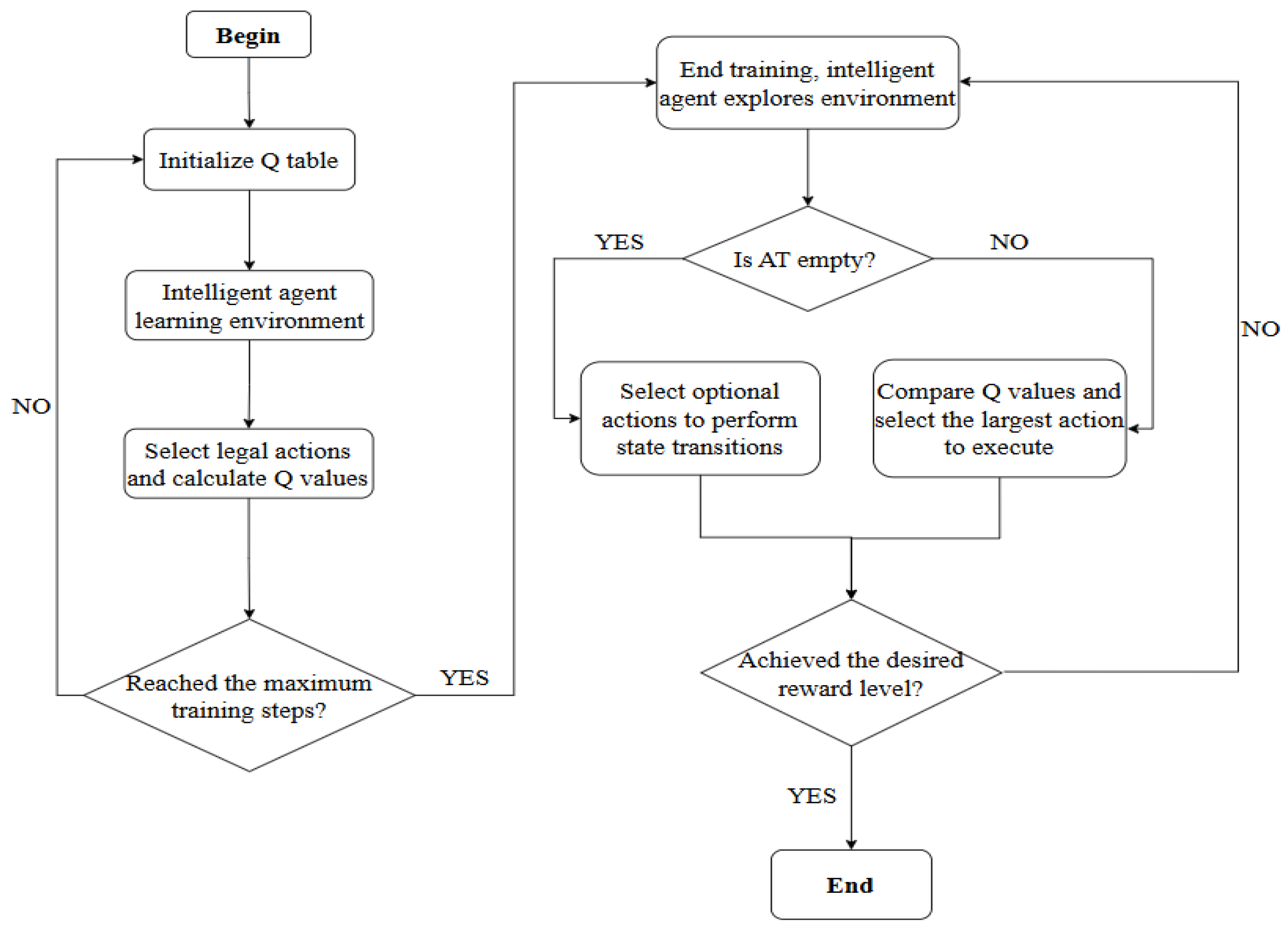
The AT mechanism demonstrates critical utility when processing state 3 after disassembly task 4, where accessible subassemblies <4> and <6> enable subsequent non-conflicting tasks 6 and 7. Selection of either task automatically preserves the alternative in the AT for future transitions, strategically expanding the search space. This innovation proves particularly valuable in large-scale industrial scenarios featuring frequent parallel non-conflicting tasks. By enabling direct retrieval of valid actions from the AT rather than restarting searches from AND/OR graph roots the approach significantly enhances global search capability while improving adaptability to concurrent operations. Consequently, training efficiency increases, convergence accelerates, and superior solutions emerge within reduced training steps. The IQ($\lambda$) algorithm flowchart is shown in Figure 5.

The steps of the IQ($\lambda$) algorithm are as follows:

• Step 1: Initialize the Q-table, the eligibility trace matrix E, the learning rate $\alpha$, the discount factor $\gamma$, and the trace decay factor $\lambda$.
• Step 2: Train the agent to become familiar with the environment. A random state is selected from the state space, and an action is randomly chosen from the action space. If the selected action is invalid, the algorithm immediately proceeds to the next learning episode. If the action is valid, the agent transitions to a new state based on the selected action and receives a corresponding reward. The value function is updated using the TD error. This process continues until a certain level of reward is achieved or no further actions are available, at which point the next learning episode begins. The process is repeated until the maximum number of training steps is reached.
• Step 3: After completing the training phase, the agent enters the deployment phase. Starting from state 1, the agent selects actions. For each decision, the agent first checks whether the action table (AT) contains any candidate actions. If so, the Q-values of those actions are compared with those of the currently available actions. The agent then selects an action according to the $\epsilon$-greedy policy and performs a state transition. Afterward, the eligibility traces are updated according to a decay rule, which gradually reduces the impact of past rewards. The agent continues selecting actions and transitioning states, comparing Q-values from both the current action space and the AT, until the cumulative reward reaches a specified threshold.
• Step 4: Perform the assembly tasks based on the assembly precedence graph. According to the principle of task similarity, similar disassembly and assembly tasks should be assigned to the same workstation whenever possible.

In summary, the IQ($\lambda$) algorithm incorporates significant improvements in both algorithmic structure and its applicability to disassembly-assembly lines. The integration of the Action Table mechanism and trace update strategy enhances the agent’s global search capability and decision efficiency. These enhancements enable the algorithm to effectively solve the DALBP studied in this work, demonstrating that value-based reinforcement learning methods, when properly improved, can be successfully applied to complex scheduling scenarios such as DALBP [26,27,28].

5. Experimental Studies

This section investigates the effectiveness of the improved IQ($\lambda$) algorithm for solving DALBP. First, the mathematical model is validated using the CPLEX solver to ensure its correctness and completeness. Then, the performance of IQ($\lambda$) is compared with several baseline algorithms, including the original Q($\lambda$) [29,30], Sarsa [31], and Q-learning [32,33]. All experiments are conducted on a computer with an Intel Core i7-10870H processor and 16 GB RAM, running Windows 10. The algorithms are implemented in Python using the Pycharm development environment.

5.1. Test Instances

This work evaluates the performance of the IQ($\lambda$) algorithm using four test cases. The test cases include a flashlight, a copying machine, an automobile battery, and a hammer drill.

Table 2. Parameters of each calculation case.

Case	Product	Number of Tasks, i.e., |$\mathbb{I}$|	Number of Subassemblies, i.e., |$\mathbb{E}$|
1	Flashlight	10	15
2	Copying Machine	13	15
3	Automobile Battery	9	16
4	Hammer Drill	46	63

summarizes the number of tasks and subassemblies. Associated with each instance [34,35].

Table 3. Results of test instances.

Case	Disassembly and Assembly Sequence	Objective Value	Running Time (s)
1	(2 → 4 → {1 → 2}) → (9 → 10) → ({3 → 4 → 5 → 6})	38.3	5.04
2	(1 → 12) → (7 → 10 → {1}) → (2) → (3 → 4 → 5)	45.4	7.63
3	(1 → 3 → {2}) → (5 → {1} → 7) → (9 → {4 → 3}) → (6 → {5})	58.1	8.27
4	——	——	——

presents the solution results obtained by the CPLEX solver for each test instance. In this table, assembly task sequences are indicated using curly braces, while parentheses denote tasks that are assigned to the same workstation. No result is provided for Case 4 because the CPLEX solver failed to find a solution for the hammer drill instance within the 3600 s time limit. Since CPLEX uses a branch-and-bound method that enumerates all possible solutions to find the optimal one, the limited memory of 16 GB on the experimental computer was insufficient to handle the large-scale instance. Consequently, CPLEX did not yield a feasible solution and reported a memory overflow issue.

5.2. Comparison

This work employs the Sarsa, Q-learning, and Q($\lambda$) algorithms as benchmarks to conduct comparative experiments with the proposed IQ($\lambda$) algorithm. The hyperparameters for the four algorithms across the four test instances are unified, as shown in

Table 4. Four algorithms: hyperparameters.

Case	Training Steps	Discount Rate $\mathit{\gamma }$	Learning Rate $\mathit{\alpha }$	Decay Factor $\mathit{\lambda }$	Action Space Size	Episodes
1	1000	0.9	0.5	0.8	10	4
2	1000	0.9	0.5	0.8	13	4
3	1000	0.9	0.5	0.8	9	4
4	8000	0.9	0.5	0.8	46	4

. Since the decay factor $\lambda$ is not involved in Sarsa and Q-learning, the number of training steps, discount rate $\gamma$, learning rate $\alpha$, action space size, and number of training episodes are kept consistent, with $\lambda$ uniformly set to 0.8 to ensure fairness in comparison.

The results demonstrate that IQ($\lambda$) consistently achieves superior solution quality and faster convergence across all test instances. While the current implementation does not yet include live IoT data streams or device coordination, the algorithm’s performance establishes a strong baseline for eventual deployment in smart disassembly environments with cyber-physical feedback.

Table 5. Comparison of objective values and running times across algorithms.

Case	IQ($\mathit{\lambda }$)		Sarsa			Q-Learning			Q($\mathit{\lambda }$)
	Obj.	Time	Obj.	Time	Gap	Obj.	Time	Gap	Obj.	Time	Gap
1	38.3	0.02	40.1	0.17	4.69%	38.3	0.07	0%	38.3	0.03	0%
2	45.4	0.02	fail	—	—	60.2	0.74	32.59%	fail	—	—
3	58.1	0.03	58.1	0.81	0%	58.1	0.26	0%	58.1	0.05	0%
4	164.8	0.28	175.4	1.14	6.43%	fail	—	—	183.6	0.95	11.41%

details the experimental results of the optimal objective values and running times for the four algorithms on the four test instances, along with their comparative differences. Analysis of Table 5 indicates that the IQ($\lambda$) algorithm demonstrates significant advantages in both objective value and computational efficiency. In Case 1, IQ($\lambda$), Q-learning, and Q($\lambda$) all found the optimal solution of 38.3; however, IQ($\lambda$) achieved a running time of 0.02 s, substantially lower than Q-learning’s 0.07 s and Q($\lambda$)’s 0.03 s. The results for Case 2 are even more striking: only IQ($\lambda$) successfully found a high-quality solution of 45.4 in 0.02 s, whereas Sarsa and Q($\lambda$) failed to find feasible solutions within the limited number of actions. Although Q-learning found a solution, its objective value of 60.2 was significantly worse than that of IQ($\lambda$), and it required more time. For Case 3, all algorithms found the same optimal solution of 58.1, but IQ($\lambda$) converged the fastest, outperforming Sarsa and Q-learning significantly. For the most challenging large-scale Case 4, IQ($\lambda$) again achieved the best performance, obtaining the best objective value of 164.8 in the shortest time of 0.28 s. While Sarsa found a solution, its quality was inferior and runtime longer; Q-learning failed to find a feasible solution; and Q($\lambda$) found a solution with an 11.41% gap in objective value compared to IQ($\lambda$) and a runtime much higher than IQ($\lambda$).

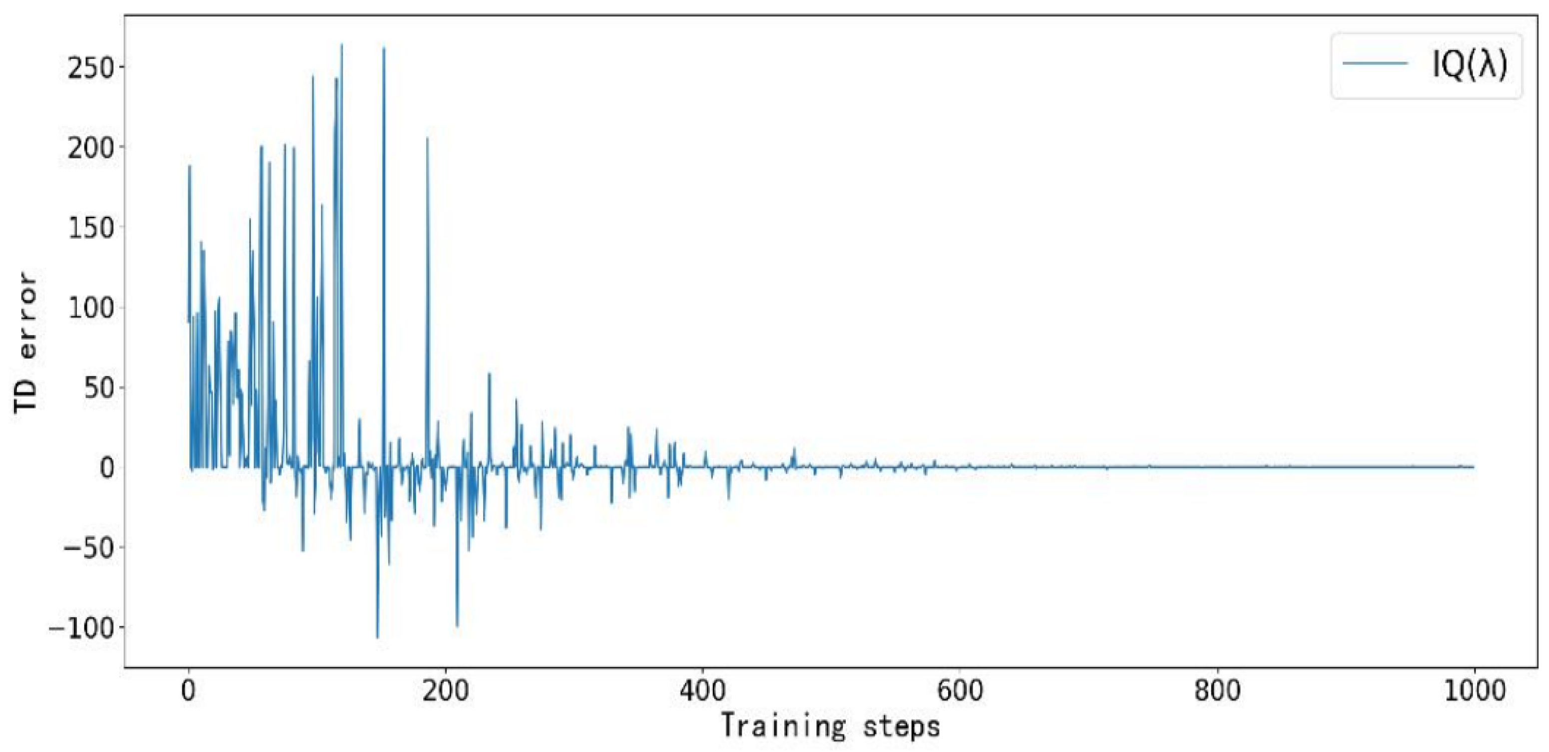
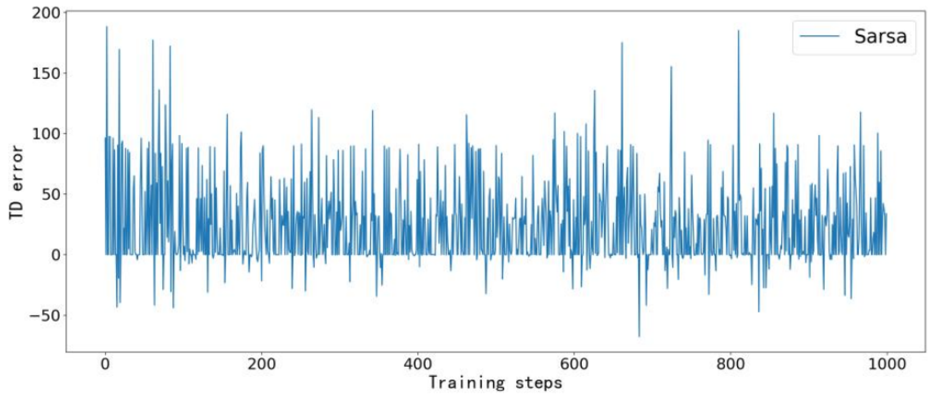
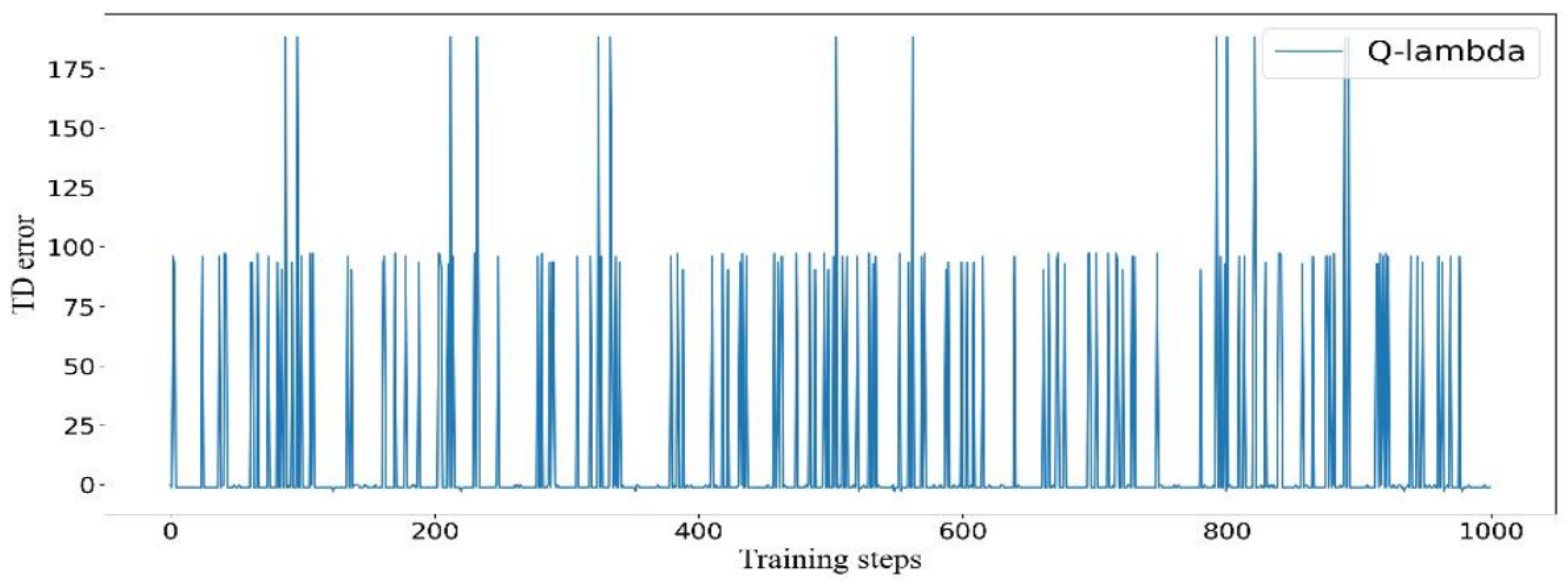
Further investigation into the convergence characteristics of the algorithms is presented in Figure 6, Figure 7, Figure 8 and Figure 9. Taking the TD error convergence process in Case 3 as an example, the IQ($\lambda$) algorithm achieves the fastest convergence, reaching a stable state after approximately 600 training steps. In contrast, Q-learning converges around step 700 but still exhibits minor fluctuations up to step 900. Sarsa and Q($\lambda$) fail to fully converge within the given number of training steps. It is worth noting that although Sarsa and Q($\lambda$) do not completely converge in Case 3, their inherent exploration behavior occasionally led them to select optimal actions by chance, thereby achieving the same optimal objective value as IQ($\lambda$). Figure 10 illustrates the reward value trajectory of IQ($\lambda$) in Case 3. During the early unstable training phase, reward values were reset to zero. The reward stabilized around step 400 and consistently maintained the optimal value of 58.1 thereafter.

Based on the above experimental findings and cross-validation against the feasible solutions provided by the commercial solver CPLEX, it can be concluded that the proposed IQ($\lambda$) algorithm exhibits significant superiority over Sarsa, Q-learning, and Q($\lambda$) in solving the DALBP addressed in this chapter. IQ($\lambda$) consistently delivers optimal or highly competitive solutions across all four test instances, with remarkable advantages in both solution quality and computational efficiency. Additionally, its convergence is the fastest and most stable among all compared algorithms, further validating the effectiveness of the algorithm design.

5.3. Melting Research and Parameter Sensitivity Analysis

To thoroughly analyze the core improvement mechanism and robustness characteristics of the IQ($\lambda$) algorithm, this section conducts ablation studies and parameter sensitivity experiments. The experimental environment and comparison algorithm settings are the same as in Section 5.2, and all results are averages of 20 independent experiments.

5.3.1. Ablation Experiment

The ablation experiments in this work aim to quantitatively evaluate the independent contributions of the three core modules—the eligibility trace mechanism ($\lambda$), the action selection table ($AT$), and the switching penalty ($\rho$)—to the algorithm’s performance. To this end, we selected Case 2 and Case 4 as test subjects, as these two cases contain different numbers of tasks, allowing us to examine the algorithm’s performance under varying levels of complexity. In the experiments, all variants used the same parameter configurations as those in Table 4. Specifically, we designed four algorithm variants for comparison: IQ($\lambda$)-Full represents the complete algorithm with all three modules; IQ($\lambda$)-NoTrace disables the eligibility trace mechanism by setting $\lambda$ to 0; IQ($\lambda$)-NoAT removes the action selection table; and IQ($\lambda$)-NoPenalty eliminates the switching penalty by setting $\rho$ to 0. The relevant experimental results are detailed in

Table 6. Melting experiment analysis.

Algorithm Variant	Copying Machine		Hammer Drill
	Target Value	Time (s)	Target Value	Time (s)
IQ($\lambda$)-Full	45.4 ± 0.0	0.02 ± 0.00	164.8 ± 2.1	0.28 ± 0.03
IQ($\lambda$)-NoTrace	48.7 ± 1.5 (+7.3%)	0.03 ± 0.01	172.3 ± 3.8 (+4.5%)	0.35 ± 0.05
IQ($\lambda$)-NoAT	47.2 ± 0.8 (+4.0%)	0.05 ± 0.01	169.5 ± 3.1 (+2.9%)	0.42 ± 0.06
IQ($\lambda$)-NoPenalty	50.1 ± 2.2 (+10.4%)	0.02 ± 0.00	181.7 ± 5.6 (+10.3%)	0.27 ± 0.04

.

The complete IQ($\lambda$) algorithm consistently achieves the lowest target values, fastest computation times, and highest stability across both scenarios. Specifically, the eligibility trace mechanism effectively reduces performance variance and improves solution quality; the action table accelerates the search process by reducing computational overhead; and the switching penalty plays a critical role in avoiding ineffective action switches and maintaining solution quality. Disabling any single module leads to clear degradation in solution quality, longer computation time, or increased instability. These results highlight the strong synergy among the modules, demonstrating that the full IQ($\lambda$) algorithm delivers significantly better overall performance.

5.3.2. Parameter Sensitivity Analysis

Parameter sensitivity analysis is conducted to investigate the effects of key algorithm parameters on performance. Specifically,

Table 7. Sensitivity analysis of $\rho$ (mean objective values).

$\mathit{\rho }$ Value	Copying Machine	Hammer Drill	Performance Trend
0.0	50.1	181.7	Frequent switching, poor solution quality
0.1	47.8	172.5
0.2	46.2	167.3	Solution quality improves with increasing $\rho$
0.3	45.6	165.1	Optimal range
0.5	45.4	164.8	Optimal range
0.7	45.9	165.7	Over-suppresses effective switching

presents the sensitivity to the switching penalty coefficient $\rho$,

Table 8. Sensitivity analysis of $\alpha$ (objective value and convergence steps).

$\mathit{\alpha }$ Value	Flashlight (10 Tasks)		Hammer Drill (46 Tasks)
	Objective Value	Convergence Steps	Objective Value	Convergence Steps
0.1	38.3	1150	168.2	>8000
0.3	38.3	850	166.5	7800
0.5	38.3	600	164.8	7200
0.7	39.1 (+2.1%)	520	173.3 (+5.2%)	6900
0.9	40.7 (+6.3%)	480	182.5 (+10.7%)	6500

shows the sensitivity of the learning rate $\alpha$ in terms of objective value and convergence steps, and

Table 9. Task scale sensitivity analysis.

Task Scale	Case Study	IQ($\mathit{\lambda }$) Advantage	Runtime
Small (≤10 tasks)	Flashlight	Matches CPLEX optimal solution	0.02 s
Medium (13 tasks)	Copying Machine	100% success rate (Q-learning fails)	0.02 s
Large (≥46 tasks)	Hammer Drill	11.4% better than Q($\lambda$)	0.28 s

illustrates the sensitivity to task scale.

• Sensitivity to switching penalty coefficient $\rho$
  Conclusion: The optimal range of $\rho$ is [0.3, 0.5]. Complex tasks (hammer drill) are more sensitive to $\rho$, achieving an 11.4% improvement in objective value when $\rho$ increases from 0.0 to 0.5.
• Sensitivity to learning rate $\alpha$
  Conclusion: $\alpha =0.5$ achieves the best trade-off between convergence speed and solution quality. When $\alpha >0.7$, convergence accelerates but objective values deteriorate significantly by more than 5%.
• Sensitivity to task scale
  Conclusion: IQ($\lambda$) demonstrates strong scalability. As the task scale increases from 13 to 46, the synergy between eligibility traces and action table becomes more significant, with runtime increasing moderately (0.02 s → 0.28 s), much slower than the growth in problem size.

6. Discussion: Implications for IoT Cybersecurity

The integration of IoT technologies into cyber-physical disassembly systems introduces both opportunities for real-time optimization and challenges related to cybersecurity and data privacy. While this work focuses on optimizing the disassembly-assembly line balancing problem (DALBP) through the improved IQ($\lambda$) algorithm, the broader context of IoT-enabled manufacturing necessitates attention to data protection, system integrity, and trust-aware decision-making.

The reinforcement learning framework proposed in this work is inherently extensible to secure and privacy-preserving architectures. In an IoT-enabled disassembly line, sensors and edge devices continuously collect and transmit data related to product conditions, task dependencies, worker safety, and robot dynamics. This data enables adaptive task planning but simultaneously raises concerns over the exposure of operational and user-sensitive information.

Building upon the modular architecture of IQ($\lambda$), the following extensions illustrate how IoT cybersecurity and privacy could be systematically incorporated:

Privacy-Aware Task Sequencing: The task selection mechanism in IQ($\lambda$), enhanced with instruction-tuned LLM guidance, can be adapted to prioritize the early disassembly of components containing sensitive or proprietary data (e.g., memory chips, identity-tagged modules). This ensures these parts are securely isolated or neutralized, reducing the risk of data leakage.

Federated Learning for Worker Privacy: In future IoT-integrated implementations, reinforcement learning agents can be combined with federated learning to enable decentralized policy updates across edge devices. Worker-related data, such as posture, fatigue, or biometric information, can be processed locally at each robotic cell, minimizing exposure and ensuring compliance with privacy regulations such as GDPR or HIPAA.

Secure Communication for Edge Devices: Edge nodes and robotic controllers in the proposed system can benefit from lightweight cryptographic protocols and attribute-based encryption schemes. These mechanisms ensure secure communication of task instructions and status updates without overburdening resource-constrained devices, maintaining the system’s real-time performance.

Trust-Aware Reward Design: The reward function in IQ($\lambda$) can be extended to incorporate trust and safety constraints. For example, task transitions that risk ergonomic overload or require exposure of identifiable worker data can be penalized. Through such design, the algorithm not only optimizes task scheduling but also upholds ethical and legal boundaries in human-robot collaboration.

Edge-AI Integration and Privacy-by-Design: Although not implemented in the current study, the architectural structure of IQ($\lambda$) supports future integration with edge-AI modules. These could enable secure inference at the sensor level, reinforcing a privacy-by-design workflow where data remains local, and only essential decision updates are propagated to the cloud.

In summary, the improved IQ($\lambda$) algorithm provides not only a robust solution for DALBP in smart manufacturing but also a foundation upon which future extensions can build to address emerging concerns in IoT cybersecurity and privacy. As disassembly lines become increasingly connected and autonomous, the intersection of optimization, learning, and secure communication will be critical to ensuring both operational efficiency and data integrity.

7. Conclusions

This paper presents an improved Q($\lambda$)-based reinforcement learning framework to solve the Disassembly and Assembly Line Balancing Problem (DALBP), with a particular focus on modeling directional switching time and conflict constraints in robotic operations. The proposed IQ($\lambda$) algorithm introduces key innovations including eligibility trace decay, a dynamic Action Table mechanism, and reward shaping that penalizes inefficient task switching. These features significantly enhance the agent’s ability to explore and optimize large-scale, parallelizable task sequences.

Through comprehensive experiments on four benchmark cases, IQ($\lambda$) demonstrates superior performance over baseline algorithms (Q-learning, Sarsa, and Q($\lambda$)) in terms of both objective value and convergence speed. Notably, the algorithm handles complex, large-scale problems such as the hammer drill case that proved infeasible for the commercial solver CPLEX.

Although the current implementation does not yet integrate real-time IoT infrastructure, the modular design of IQ($\lambda$) is specifically tailored to enable future deployment in IIoT-based smart factories. This includes potential extensions involving federated learning, privacy-preserving task planning, lightweight cryptographic communication, and trust-aware optimization. As industrial systems evolve toward interconnected and autonomous paradigms, the proposed approach offers a practical, scalable foundation for secure and efficient robotic scheduling under cyber-physical conditions.

Future work will focus on embedding the algorithm into an edge-enabled disassembly system, incorporating live sensor feedback, cyber defense measures, and cloud-based policy refinement, with the goal of advancing secure and adaptive learning in IoT-driven manufacturing environments.