Article

A High-Payload Data Hiding Method Utilizing an Optimized Voting Strategy and Dynamic Mapping Table

1
Department of Computer Science and Information Engineering, Asia University, Taichung 41354, Taiwan
2
Department of Information Management, Lunghwa University of Science and Technology, Taoyuan 33306, Taiwan
3
Department of Artificial Intelligence, Asia University, Taichung 402, Taiwan
4
Department of Medical Research, China Medical University Hospital, China Medical University, Taichung 40402, Taiwan
*
Author to whom correspondence should be addressed.
Electronics 2025, 14(17), 3498; https://doi.org/10.3390/electronics14173498
Submission received: 10 July 2025 / Revised: 28 August 2025 / Accepted: 29 August 2025 / Published: 1 September 2025
(This article belongs to the Special Issue Advances in Cryptography and Image Encryption)

Abstract

The exponential growth of multimedia communication necessitates advanced techniques for secure data transmission. This paper details a new data hiding method centered on a predictive voting mechanism that leverages neighboring pixels to estimate a pixel’s value. Secret data are concealed within these predictions via a purpose-built lookup table, and the retrieval process involves re-estimating the predicted pixels and applying an inverse mapping function. Experimental results demonstrate that the proposed method achieves an embedding capacity of up to 686,874 bits, significantly outperforming previous approaches while maintaining reliable data recovery. Compared with existing schemes, our approach offers improved performance in terms of both embedding capacity and extraction accuracy, making it an effective solution for robust multimedia steganography.

1. Introduction

The swift progress of IT, especially the widespread use of 5G, has fueled the expansion of cloud storage and computing. Because cloud tech offers many benefits, more and more people are opting to keep their data, particularly multimedia like photos, audio, and videos, on cloud services. However, since these data often travel over public networks or reside on distant cloud servers, their security and dependability are not always certain. Consequently, safeguarding these data has become a critical concern for researchers and industry experts alike. Steganography offers various ways to hide information. One basic approach is to directly embed each bit of secret data into the cover medium. Another strategy involves selectively embedding data in noisy or complex areas of the cover to make them harder to detect. Some techniques also spread hidden data randomly throughout the cover. Digital images are a vital way to represent data and are essential in fields like photography, defense, medicine, and law. Within data security, hiding information within images has become a significant research focus. An image data hiding (DH) system works by embedding secret data into a cover image. The goal is to create a modified image, called a stego-image, where the alterations caused by the hidden data are imperceptible to human vision. Image data hiding systems typically involve two essential parts: the secret information being concealed and the original image used as a disguise. The secret data are embedded into the original image, resulting in a modified image called a stego-image. This process aims to make any changes to the image virtually invisible. These systems are used in two main ways. In the first scenario, the primary goal is to protect the hidden data, and there is no need to recover the original image. In the second scenario, both the hidden data and the original image are crucial and must be perfectly restored by the recipient, which is particularly important in areas like defense and healthcare. The first approach, where the original image cannot be recovered, is called irreversible data hiding. The second approach, which allows for the complete recovery of both the hidden data and the original image, is known as reversible data hiding (RDH) [1,2].
In recent surveys [3], Ragab et al. emphasized the growing significance of image steganography and RDH, particularly for sensitive domains such as medical and military imaging. Unlike conventional steganography, RDH ensures the recovery of both secret data and the original image, enhancing applicability where fidelity is crucial. While the review highlights advancements in encrypted and compressed domains and addresses steganalysis threats, many approaches still face trade-offs between capacity, robustness, and computational efficiency.
Common steganographic methods range from simple least significant bit (LSB) substitution and masking techniques to more sophisticated methods that use algorithms and transformations like the discrete cosine transform (DCT) or discrete wavelet transform (DWT) [4]. Data security relies on several methods, such as concealing information (data hiding) [5], scrambling it (encryption) [6], creating a unique fingerprint (hashing) [7], distributing it among multiple parties (secret sharing) [8] and Histogram shifting(HS) [9], prediction-based DH (PDH) [10], and pixel value ordering (POV) [11].
Histogram shifting (HS) starts by looking at how often each brightness level appears in an image. Then, it adjusts this “brightness map” a bit to make space for hidden information that can be undone later. Both PDH and PVO cleverly hide data in images by making small changes to pixel brightness, allowing for later retrieval of the secret and (in PVO’s case) the original image. PDH predicts pixel values to embed data, while PVO sorts pixel brightness in small blocks and modifies the extremes. PDH methods are sensitive to the accuracy of pixel estimation and the data embedding process. The effectiveness of these techniques, in terms of performance and image quality, hinges on selecting a suitable prediction model (like median edge detector, rhombus predictors, or interpolation-based methods) [12,13] that can precisely estimate pixels targeted for data embedding.
Yavuz [14] introduced a reversible data hiding in encrypted images that combined chaos theory with the Chinese remainder theorem, offering a fixed embedding capacity (0.5 BPP) and semi-separability. While the method ensures strong cryptographic security and robustness, its reliance on pixel fusion and fixed capacity may limit its adaptability compared to adaptive or learning-based approaches. Nonetheless, it demonstrates competitive performance against several state-of-the-art techniques. Hybrid steganographic methods that use compression, adaptive embedding, and deep learning are very good at hiding data without making visible changes and can resist noise and compression. However, these methods are often slow, require a lot of data for training, and do not work well on different types of images. This shows that there is a need for simpler but secure methods [15]. Recent works have explored deep learning in steganography, with generative adversarial network and DWT-based models showing improved invisibility compared to conventional methods. The integration of multi-scale attention and patch-based discriminators enhances feature embedding and detection resistance. However, despite achieving superior performance on benchmark datasets, these approaches often involve high computational cost and may face challenges in practical deployment [16].
Furthermore, the data embedding strategy must be carefully designed and optimized to reduce image distortion for a given amount of hidden data. In 2024, Chi et al. [17] proposed a data hiding scheme that uses a voting-based prediction strategy, modifying predicted pixel values directly to embed secret data. It maintains fixed seed pixels for prediction, with image quality largely dependent on prediction accuracy. Each predicted pixel can embed up to 7 bits of data, with greater data amounts requiring larger modifications. In their proposed method, they have a low embedding capacity; as the value of the predicted pixel increases beyond a specific limit, their method fails to embed the data.
In this article, we propose an improved scheme in which the embedding capacity of the data increases and more pixels are used for data hiding. The novel scheme combines a voting-based pixel prediction method with a lookup-table-guided embedding strategy. This fusion enables a high-capacity, low-distortion, and fully reversible data hiding technique.
The article can be divided into the following sections: Section 2 presents the related work, Section 3 explains the detailed proposed methodology, Section 4 highlights the experimental results, and Section 5 presents the conclusion.

2. Related Works in Neighborhood Pixel Technique

A reversible data hiding technique called neighbor mean interpolation (NMI) was developed by Jung and Yoo [18]. While this method excels at producing stego-images with excellent visual quality, it does not allow for embedding a large amount of data.
Traditional interpolation methods usually calculate the value of a pixel by considering its four immediate neighboring pixels. When applying interpolation for data hiding, the common procedure involves the following steps:
  • First, an original image I of size X × Y is down-scaled to a smaller image with dimensions X 2 × Y 2 .
  • Next, this reduced image is divided into overlapping 2 × 2 blocks. These blocks are then processed sequentially in a raster scan order, which is similar to reading text from left to right and top to bottom, as shown in Figure 1a.
  • Following the downscaling and block segmentation, each 2 × 2 block is expanded into a 3 × 3 overlapping block. In this enlarged block, the pixel positions that were omitted during the down scaling process are reconstructed using interpolation techniques. Figure 1b visually illustrates this concept: the original seed pixels from the 2 × 2 block are shown in green, while the white regions represent the positions where new, interpolated pixel values must be computed.
Specifically, the neighbor mean interpolation method, introduced by Jung and Yoo [18], calculates the missing pixel values by averaging adjacent seed pixels. Equation (1) outlines this computation:
M ( 1 , 0 ) = M ( 0 , 0 ) + M ( 2 , 0 ) 2 , M ( 0 , 1 ) = M ( 0 , 0 ) + M ( 0 , 2 ) 2 , M ( 1 , 1 ) = M ( 0 , 0 ) + M ( 2 , 0 ) + M ( 0 , 2 ) 3 .
The pixel M ( 1 , 0 ) is estimated by averaging its horizontal neighbors from the original 2 × 2 block, M ( 0 , 1 ) is calculated by averaging its vertical neighbors, and M ( 1 , 1 ) is determined by averaging the three surrounding original pixels. Lee and Huang developed the interpolated by neighborhood pixel (INP) technique [19], which offers a different approach to image interpolation compared to the standard nearest neighbor interpolation (NNI). A key distinction of INP is its emphasis on the top-left pixel, M ( 0 , 0 ) , which gives it more weight in the calculation. To estimate the pixel value at M ( 1 , 1 ) , INP calculates two intermediate interpolated values and then averages them, as shown in Equation (2) and visually represented in Figure 1.
The value of M ( 1 , 0 ) is computed as the average of M ( 0 , 0 ) and M ( 2 , 0 ) :
M ( 1 , 0 ) = M ( 0 , 0 ) + M ( 0 , 0 ) + M ( 2 , 0 ) 2 2 , M ( 0 , 1 ) = M ( 0 , 0 ) + M ( 0 , 0 ) + M ( 0 , 2 ) 2 2 , M ( 1 , 1 ) = M ( 1 , 0 ) + M ( 0 , 1 ) 2 .
This method prioritizes the contribution of the central pixel M ( 0 , 0 ) during the interpolation, which can lead to improved visual quality in the resulting image.

3. The Proposed Scheme

This section presents an improved method for hiding data within images. It works by first estimating pixel values using a voting strategy, where multiple neighboring pixels contribute to the prediction. Then, the secret data are embedded into the image based on specific mapping, as shown in Table 1, which links data bits to pixel modifications. Before embedding the data, the following steps are performed:
  • Step 1:The original P × Q image, I, is segmented into a checkerboard pattern where white pixels serve as unaltered reference seeds, and blue pixels are designated for embedding secret information. The value of each blue pixel (P) is predicted solely based on its four neighboring white pixels ( a 1 , a 2 , a 3 , and a 4 ), which denote the left, upper, right, and lower pixel of the pixel, respectively.
  • Step 2: The value of a central pixel P is determined by looking at the values of its four surrounding pixels. This prediction process has five different scenarios, which are shown in Figure 2:
    Scenario 1 (uniform neighbors): If all four neighboring pixels have the exact same value, then P is assigned that value.
    Scenario 2 (two matching pairs): If the four neighbors form two pairs of identical values, then P is predicted as the average of one of these pairs.
    Scenario 3 (one matching pair): If only one pair of neighboring pixels has the same value, then P is assigned the value that appears most frequently among the four neighbors.
    Scenario 4 (three identical neighbors): If three of the four neighbors share the same value, then P takes on that majority value.
    Scenario 5 (all different neighbors): If all four neighboring pixels have distinct values, then P is calculated as the average of these four values.
    P = a 1 , if a 1 = a 2 = a 3 = a 4 ( Uniform Neighbors ) , a 1 + a 3 2 , if ( a 1 = a 2 ) ( a 3 = a 4 )   ( Two   Matching   Pairs ) , mode ( a 1 , a 2 , a 3 , a 4 ) , if   exactly   one   pair   of   neighbors   are   equal , a 1 , if   a 1 = a 2 = a 3 a 4       ( Three Identical   Neighbors ) , a 1 + a 2 + a 3 + a 4 4 , if   all   four   neighbors   are   distinct .
  • Step 3: When dealing with pixels along the edges or at the corners of an image, there are fewer neighboring (seed) pixels to reference. As a result, the prediction approach adapts accordingly:
    (1) For edge pixels (where three seed pixels are available), if all three seed pixels have the same value, use Prediction Type 1; if any two of the seed pixels have the same value, use Prediction Type 4; if all three seed pixels have different values, use Prediction Type 5.
    (2) For corner pixels (where two seed pixels are available), if the two seed pixels are identical, use Prediction Type 1; if the two seed pixels have different values, use Prediction Type 5.
In summary, the prediction of a pixel’s value based on its neighbors employs several distinct approaches depending on the consistency of the surrounding pixels. If all neighboring pixels share an identical value, that value is simply replicated. When two pairs of neighboring pixels have matching values, the prediction becomes the average of one of these identical pairs. In scenarios where only two neighboring pixels match, the value that appears more frequently among the neighbors is selected. Suppose three of four neighboring pixels hold the same value; then, the dominant value is used for prediction. Finally, when all four neighboring pixels exhibit unique values, their average is calculated and utilized as the predicted value.

3.1. Data Embedding Phase

After the preprocessing steps, the next phase is to embed the data. The steps of the improved method are as follows:
  • Step 1: Begin by calculating the estimated value, P, of the pixel. For the Scenario 2 prediction, P is determined by taking the average of two adjacent pixels that have similar values. In this case, the neighboring pixel values are 15 and 16. Then, compute their average.
  • Step 2: A secret message consisting of T bits is prepared to be embedded into the pixel.
  • Step 3: Now, we need to check the mapping table to determine how much we need to adjust our initial prediction, P. In this step, the embedding process adjusts the anticipated pixel value based on a lookup table, as shown in Table 1. Initially, a group of T secret bits is translated into its decimal equivalent, D, which serves as a compact integer representation of the hidden data. For example, the bit sequence “010” becomes D = 2 .
    Next, this decimal value is mapped to an offset, Δ , using the predefined lookup table. Each value of D { 0 , 1 , , 9 } has a unique corresponding offset from the range { 5 , 4 , 3 , 2 , 1 , 0 , + 1 , + 2 , + 3 , + 4 } . This mapping guarantees that every potential secret data value leads to a specific pixel modification.
    Finally, the anticipated pixel, P, is modified by the chosen offset to create the stego-pixel, denoted as P = P + Δ . For instance, as depicted in Figure 3, the predicted pixel value is calculated as follows:
    P = 15 + 16 2 = 15 .
    When the secret bits “010” are embedded, their decimal form is D = 2 , which corresponds to an offset of Δ = + 1 . Consequently, the stego-pixel is derived as P = 15 + 1 = 16 , and the modified block is updated in the stego-image. This method ensures that each group of secret bits reliably generates a unique alteration to the predicted pixel value, facilitating both consistent data embedding and precise extraction.
  • Step 4: Modify the predicted pixel values according to Table 1 and form the stego-image. Figure 3 represents an example of the embedding process.

3.2. Data Extraction Phase

The hidden data can be extracted from the stego-image by applying the inverse of the embedding method, which is also shown in Figure 4. The following are the steps of the extraction process:
  • Step 1: The stego-image is split into two distinct categories, similar to the embedding process. Blue pixels hold the concealed secret information. White pixels remain unchanged from the original image and function as reference or seed pixels. The pixel, P’, falls into the gray pixel category, meaning it contains the embedded secret data.
  • Step 2: To retrieve the hidden secret data, we start by estimating P, which represents the pixel’s original value before the data were embedded. The method of prediction is selected based on the values of the four adjacent seed pixels.
  • Step 3: We estimate the original value of the current pixel P as P. Then, using the difference between P and P, we refer to the mapping table to determine the corresponding decimal secret value D. Finally, this decimal value D is converted into a T-bit binary number, S 1 , S 2 , , S T , where T { 1 , 2 , , 5 } .
  • Step 4: When the extracted secret data are retrieved, we reverse the modification and obtain the original pixel value, P.

3.3. Overflow and Underflow

In image processing with eight-bit unsigned integers (where pixel values range from 0 to 255), overflow occurs when a calculated pixel value increases above 255. Depending on how the system handles this, the value might wrap around (e.g., 256 becomes 0) or be clamped (limited) to 255. Underflow happens when a calculated pixel value drops below 0. Similarly, the system might wrap around (e.g., −1 becomes 255) or be clamped (limited) to 0, potentially causing data loss or display errors.
To avoid pixel values going out of the acceptable 0–255 range (overflow or underflow), a check must be performed before hiding any secret data in a pixel. This check looks at whether using the smallest or largest values from our k-bit mapping table with the predicted pixel value would push it beyond the valid limits. If this check reveals a possible overflow or underflow, we do not embed any data in that pixel and instead leave it as it was originally. Each predicted pixel P is modified using the mapping table, which shifts its value based on the secret data. The possible modifications range from P 4 (left extreme) to P + 3 (right extreme). To prevent overflow/underflow, we must check whether these extreme values remain within the valid range (0–255).
Example: If S = 3 (three-bit secret data), the mapping table allows changes from P 4 to P + 3 . Before embedding, check the following:
P 4 0 ,
P + 3 255 .
The general formula we proposed in our method is as follows.
If T = n (n-bit secret data), the following are true:
  • Case 1: 4 P n
    The embedding and extraction methods are the same as the method of Chi et al. [17].
  • Case 2: n P
    -
    Embedding: If S ( P = P + i 256 ), then P = P + i n .
    -
    Extraction: If P < P n , then P = P + n P = P + i S .
  • Case 3: P n
    -
    Embedding: If S ( P = P i 0 ), then P = P i + n .
    -
    Extraction: If P > P + n , then P = P n P = P + i S .
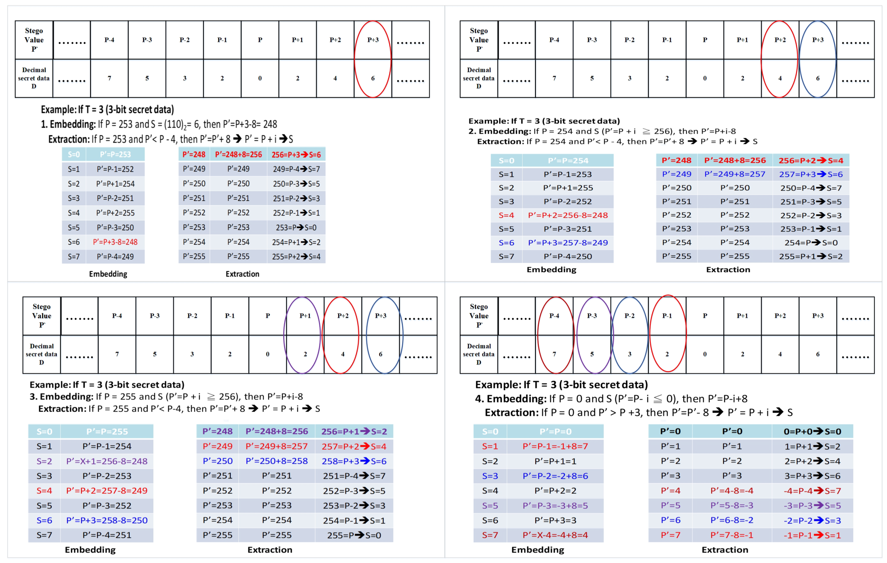
Figure 5 illustrates a steganographic data hiding method for embedding three-bit secret data (values 0–7) into pixel values using modular arithmetic, specifically when the threshold T = 3 . Four edge cases are shown based on the pixel value P: near the upper bound ( P = 253 , 254 , 255 ) and the lower bound ( P = 0 ). The embedding process adjusts P by adding or subtracting offsets (including + 8 or 8 ) to produce a modified stego-value P , ensuring the secret data can be embedded without exceeding pixel limits (0–255). When P is near the maximum (e.g., 255), values may wrap around, and when P is near zero, underflow is handled similarly. During extraction, the method reverses the embedding logic by checking conditions, such as whether P is greater or less than P ± 4 , and applies the appropriate formula to retrieve the secret value S.

4. Evaluation Metrics

The following metrics are used to evaluate the proposed methodology, and the results show that the scheme has a better embedding capability compared to previous schemes.

4.1. Embedding Capacity

This metric quantifies the total embedding capacity, representing the number of secret bits contained within the host image. It is formally defined in Equation (3), where the embedding rate, expressed in bits per pixel (bpp), is determined by dividing the total count of embedded bits by the overall pixel count of the cover image.
b p p = Number of Bits Embedded Number of Pixels in the Cover Image .

4.2. Peak Signal-to-Noise Ratio (PSNR)

PSNR measures the similarity between two images in terms of decibels (dB). It is calculated using Equation (4):
PSNR = 10 · log 10 MAX 2 MSE .
The mean squared error (MSE) between the cover image (CI) and the stego-image (SI) is defined by Equation (5):
MSE ( CI , SI ) = 1 O P k = 1 O l = 1 P C ( k , l ) S ( k , l ) 2 .
Here, O and P represent the dimensions of the image, while C ( k , l ) and S ( k , l ) are the pixel values of the cover and stego-images, respectively.
The comprehensive comparison in Table 2 reveals the significant advancements of the proposed method over Chi et al.’s [17] method in terms of the embedding capacity (EC), peak signal-to-noise ratio (PSNR), and structural similarity index (SSIM). Tested on standard images like Lena and Baboon across thresholds (from T = 2 to T = 5), our method consistently achieves a higher EC, demonstrating its superior ability to embed more data. What is more, despite this increased capacity, the proposed method largely maintains or even improves the image quality, which is reflected in its generally higher or comparable PSNR values. Its SSIM values are also predominantly superior, particularly at lower thresholds, indicating better visual fidelity. In essence, the proposed method offers substantial improvements that refer to the significant quantitative gains our method achieves over Chi et al.’s approach [17] by effectively balancing increased data capacity with the preservation of image quality. As detailed in Table 2, our technique provides a higher EC, reaching up to 686,874 bits, while also maintaining or improving PSNR and SSIM values. These metrics are standard for evaluating steganography and image processing, and they objectively demonstrate the superior trade-off between embedding capacity and visual quality. The proposed method “effectively balances the increase in data capacity with the preservation of image quality”. This means that we can embed a much larger amount of data without causing noticeable visual degradation. For instance, our PSNR values remain consistently above a certain threshold (e.g., 40 dB) and SSIM values stay close to 1.0. Therefore, the proposed technique achieves a strong balance between a high embedding capacity and maintained image quality, making it a promising approach for secure and efficient data hiding. The method demonstrates robust adaptability across different image types and payload sizes, outperforming existing methods in most metrics.
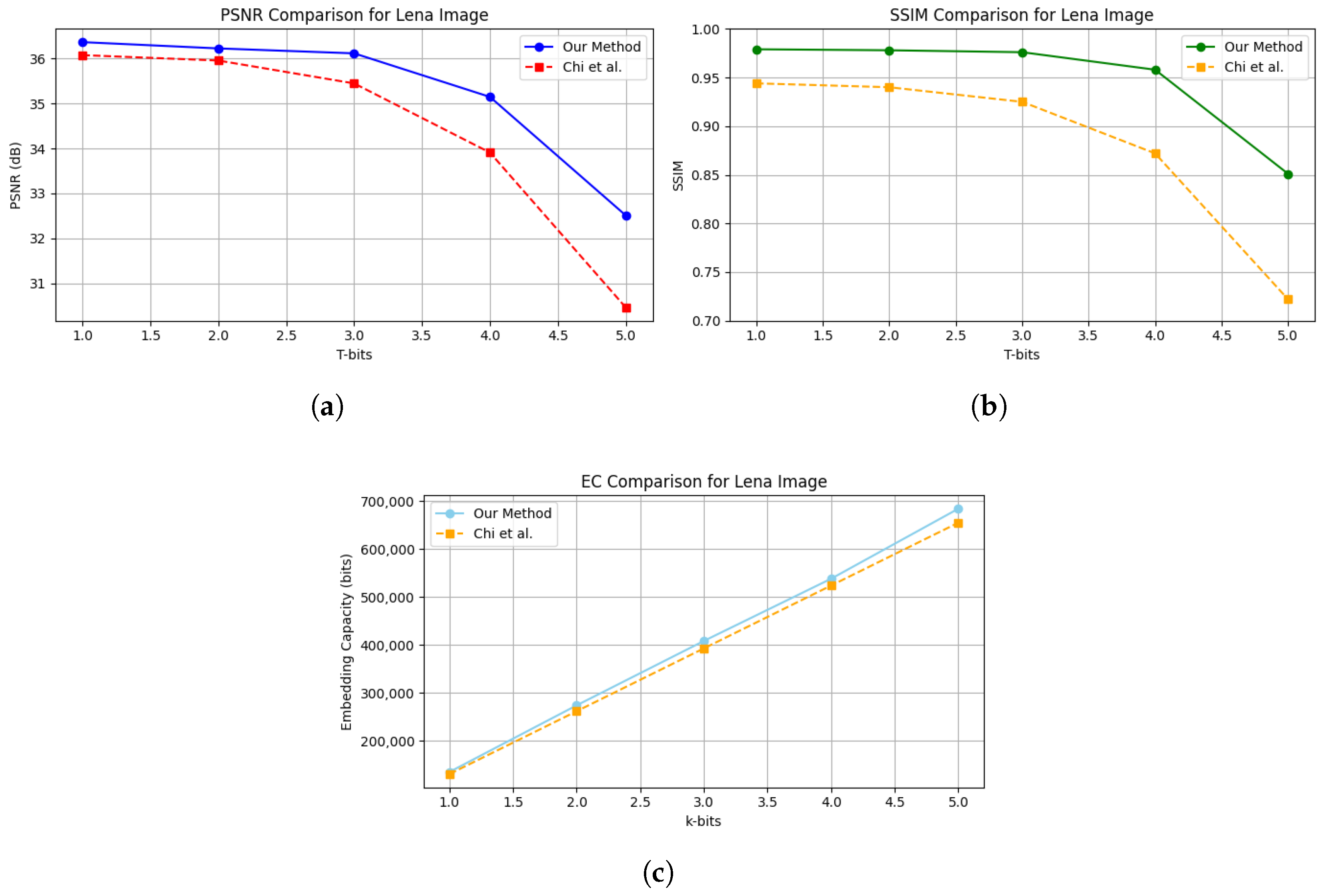
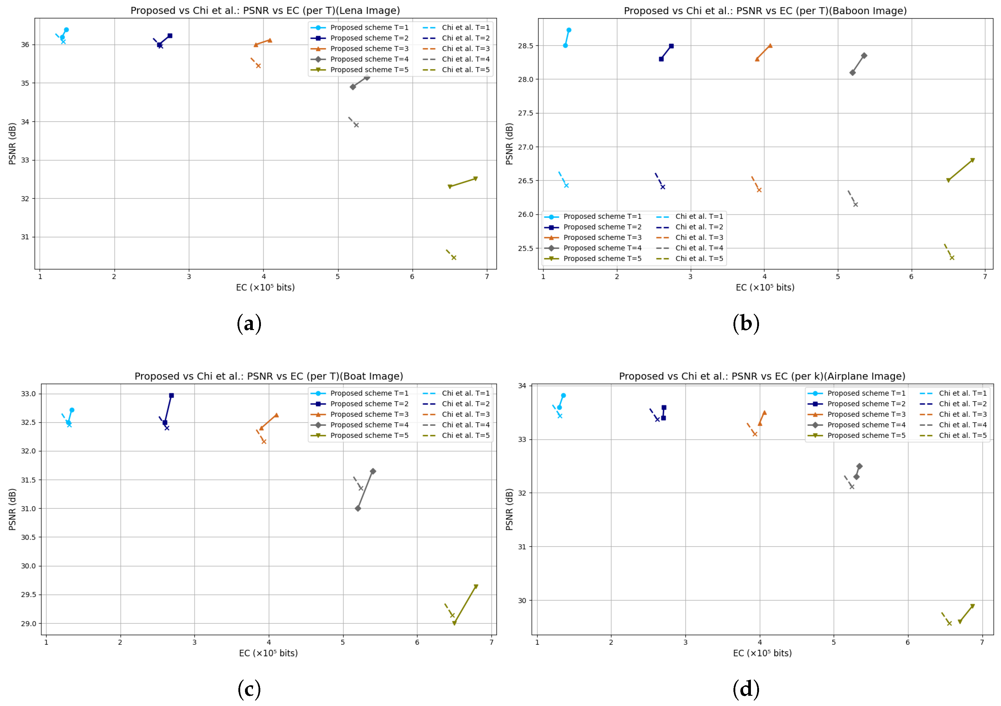
Figure 6 illustrates a comparative analysis of EC and PSNR between the method proposed in this work and that of Chi et al. [17] across six standard test images: Lena, Boat, Couple, Airplane, Baboon, and Pepper. Figure 7 and Figure 8 present a detailed comparison between the proposed method and Chi et al.’s method for the Lena and Airplane images across varying values of T-bit secret data (from 1 to 5). Figure 7a and Figure 8a show the PSNR trend, where the proposed method maintains comparable or slightly improved PSNR values as T increases. Figure 7b and Figure 8b display SSIM values, indicating that the proposed method consistently achieves higher structural similarity, suggesting better image fidelity. Figure 7c and Figure 8c illustrate the EC, where the proposed method outperforms the method of Chi et al. across all T values, demonstrating improved data hiding capability without sacrificing visual quality. Figure 9 illustrates the comparison of PSNR versus EC across different values of T (from T = 1 to T = 5) for four standard images: Lena, Baboon, Boat, and Airplane. Each subplot contrasts the proposed method (solid arrows) with Chi et al.’s method (dashed arrows) at each T level. The plots show that the proposed scheme generally achieves higher PSNR at comparable or higher EC values, indicating superior visual quality preservation while embedding more data. The consistent upward and rightward shifts of the proposed method across T values highlight its efficiency and robustness in balancing fidelity and capacity.
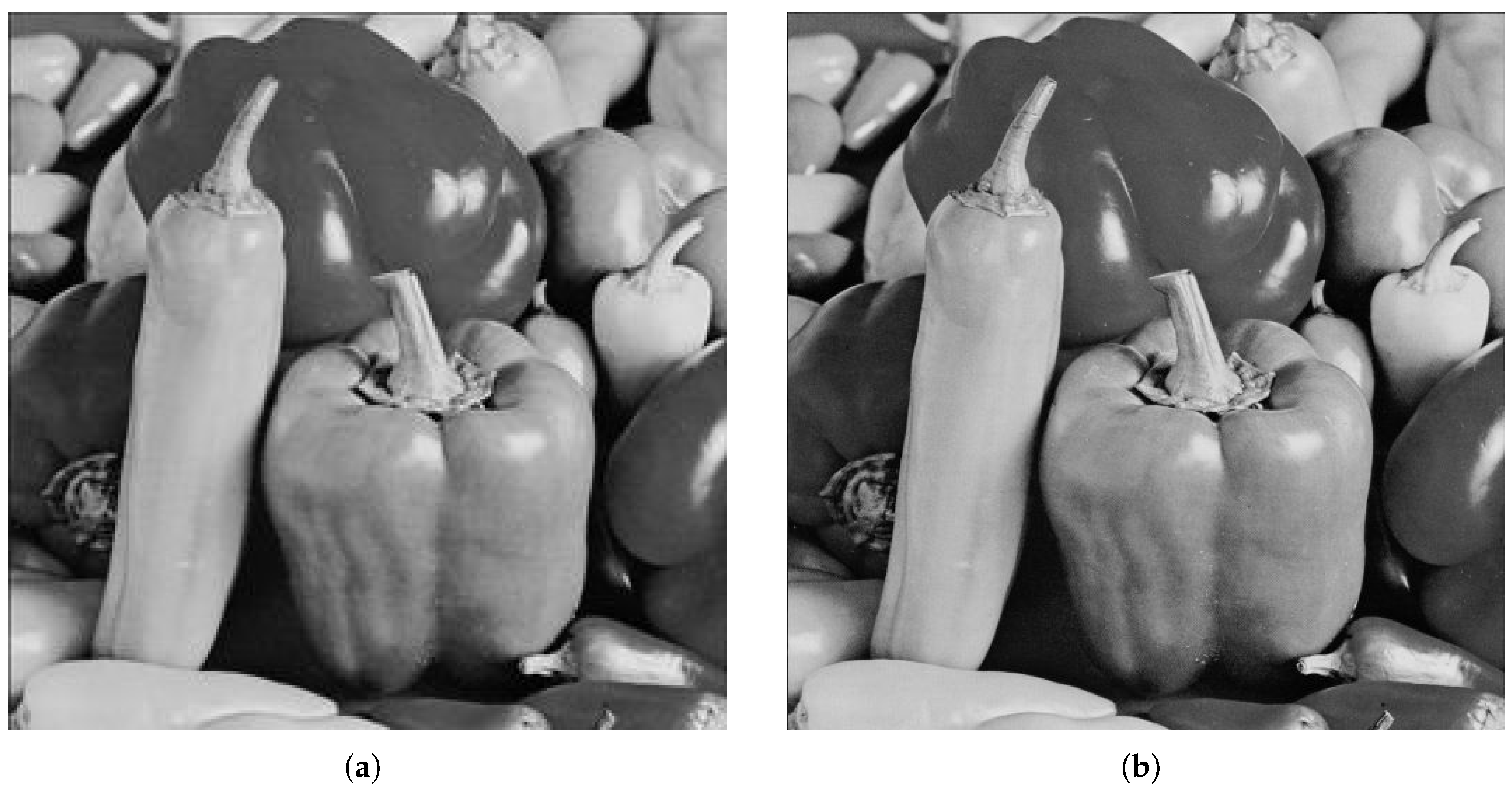
Table 3 highlights the comparison of PSNR with different methods, showing that our research has a higher PSNR than other methods. Figure 10 shows a visual comparison between the original cover image (a) and the corresponding stego-image (b) after data embedding. The figure illustrates the imperceptibility of the embedding process, showing that the stego-image closely resembles the original image with minimal visual distortion.
Also, the proposed method’s computational complexity is determined by two main operations: neighborhood voting for pixel prediction and lookup table mapping for embedding and extracting data. Both are lightweight, relying on simple integer math and table indexing, which makes our method very efficient.
Unlike deep learning approaches, our method avoids heavy training or model inference, which significantly cuts down on overhead. Our experiments on standard images (like the Lena and Baboon images) confirm that both embedding and extraction can be carried out in real time on a standard desktop, with no need for special hardware. Since the algorithm only performs local calculations and uses a fixed-size lookup table, its complexity scales linearly with the number of pixels in the image. This means the method remains efficient even with high-resolution images. Ultimately, our scheme strikes a great balance between embedding performance and computational efficiency, making it ideal for practical applications that require both speed and low complexity.
The proposed data hiding technique has broad applications in real-world scenarios that demand both a high embedding capacity and imperceptibility. For example, in medical imaging, the method can embed critical patient information or authentication codes directly into images, ensuring the integrity of diagnostic data. Similarly, in military communications, this method’s ability to conceal large amounts of sensitive data while remaining undetectable makes it ideal for secure and covert exchanges. Despite its strengths, the method has certain limitations. Its robustness may be compromised in highly dynamic or lossy environments where images undergo aggressive compression, scaling, or filtering. Furthermore, the computational cost of the prediction and lookup operations could be a constraint for real-time applications on devices with limited resources.

4.3. Security of Proposed Scheme

By making sure that the changes made during embedding are both small and statistically insignificant, the suggested approach shows resilience to steganalysis. By employing prediction-based embedding, where pixel values are estimated using local neighborhood information, the introduced changes closely follow the natural image structure. This minimizes observable abnormalities in statistical distributions, such as histograms, which are frequently exploited by steganalysis methods like RS analysis or chi-square tests. Additionally, no noticeable artifacts or unusual patterns are generated because the embedding process adaptively distributes modifications based on the local pixel context, retaining good visual quality and uniformity in structural elements. The technique thereby improves the security of the concealed communication by providing more resilience against both visual inspection and statistical steganalysis.

5. Conclusions

This article introduces a refined data hiding scheme leveraging voting-based pixel value prediction. This research introduces a novel approach that combines a voting-based pixel prediction method with a lookup-table-guided embedding strategy. This fusion enables a high-capacity, low-distortion, and fully reversible data hiding technique. Initially, a voting mechanism is employed to estimate pixel intensities. Subsequently, secret data are directly embedded into the predicted pixel values via a predefined look-up table. The extraction process involves reapplying the identical voting strategy to predict pixel intensities. The embedded data are recovered by analyzing the residual between the predicted and stego-pixel values, which is then inversely mapped using the look-up table to retrieve the original T-bit binary sequence. The proposed approach enhances both the prediction method and the data embedding strategy by considering the amount of data being hidden. Our improved scheme outperforms in (EC, PSNR, and SSIM. It allows the technique to maintain a relatively high PSNR, even when only a small amount of data are embedded.

Author Contributions

K.F. proposed the idea and wrote this paper; N.-I.W. and C.-S.C. discussed and reviewed the methodology and manuscript; M.-S.H. discussed, supervised, and reviewed the methodology and manuscript. All authors have read and agreed to the published version of the manuscript.

Funding

The National Science and Technology Council, Taiwan (ROC), partially supported this research under contract no.: NSTC 113-2221-E-468-016.

Data Availability Statement

No new data were created or analyzed in this study. Data sharing is not applicable to this article.

Conflicts of Interest

The authors declare no conflicts of interest.

References

  1. Fang, G.; Wang, F.; Zhao, C.; Chang, C.C.; Lyu, W.L. Reversible data hiding based on chinese remainder theorem for polynomials and secret sharing. Int. J. Netw. Secur. 2025, 27, 4. [Google Scholar]
  2. Ren, F.; Zeng, M.M.; Wang, Z.F.; Shi, X. Reversible data hiding in encrypted binary images based on improved prediction methods. Int. J. Netw. Secur. 2025. Available online: http://ijns.jalaxy.com.tw/contents/ijns-v99-n6/ijns-2099-v99-n6-p28-0.pdf (accessed on 28 August 2025).
  3. Ragab, H.; Shaban, H.; Ahmed, K.; Ali, A.-E. Digital image steganography and reversible data hiding: Algorithms, applications and recommendations. J. Image Graph. 2025, 13, 1. [Google Scholar] [CrossRef]
  4. Johnson, N.F.; Jajodia, S. Exploring steganography: Seeing the unseen. Computer 1998, 31, 26–34. [Google Scholar] [CrossRef]
  5. Du, Y.; Yin, Z.; Zhang, X. High capacity lossless data hiding in jpeg bitstream based on general vlc mapping. IEEE Trans. Dependable Secur. Comput. 2020, 19, 1420–1433. [Google Scholar] [CrossRef]
  6. Xian, Y.; Wang, X.; Teng, L. Double parameters fractal sorting matrix and its application in image encryption. IEEE Trans. Circuits Syst. Video Technol. 2021, 32, 4028–4037. [Google Scholar] [CrossRef]
  7. Liang, X.; Tang, Z.; Wu, J.; Li, Z.; Zhang, X. Robust image hashing with isomap and saliency map for copy detection. IEEE Trans. Multimed. 2021, 25, 1085–1097. [Google Scholar] [CrossRef]
  8. Yan, X.; Lu, Y.; Yang, C.-N.; Zhang, X.; Wang, S. A common method of share authentication in image secret sharing. IEEE Trans. Circuits Syst. Video Technol. 2020, 31, 2896–2908. [Google Scholar] [CrossRef]
  9. Chen, Y.-Y.; Hsia, C.-H.; Kao, H.-Y.; Wang, Y.-A.; Hu, Y.-C. An image authentication method for secure internet-based communication in human-centric computing. J. Internet Technol. 2020, 21, 1893–1903. [Google Scholar]
  10. Liu, L.; Wang, A.; Chang, C.-C. Separable reversible data hiding in encrypted images with high capacity based on median-edge detector prediction. IEEE Access 2020, 8, 29639–29647. [Google Scholar] [CrossRef]
  11. He, W.; Cai, Z.; Wang, Y. Flexible spatial location-based pvo predictor for high-fidelity reversible data hiding. Inf. Sci. 2020, 520, 431–444. [Google Scholar] [CrossRef]
  12. Geetha, R.; Geetha, S. Efficient rhombus mean interpolation for reversible data hiding. In Proceedings of the 2018 3rd IEEE International Conference on Recent Trends in Electronics, Information & Communication Technology (RTEICT), Bangalore, India, 18–19 May 2018; pp. 1007–1012. [Google Scholar]
  13. Huang, C.-T.; Lin, C.-Y.; Weng, C.-Y. Dynamic information-hiding method with high capacity based on image interpolating and bit flipping. Entropy 2023, 25, 744. [Google Scholar] [CrossRef]
  14. Yavuz, E. Reversible data hiding in encrypted images using chaos theory and Chinese Remainder Theorem. Pattern Anal. Appl. 2025, 28, 120. [Google Scholar] [CrossRef]
  15. Sanjalawe, Y.; Al-E’mari, S.; Fraihat, S.; Abualhaj, M.; Alzubi, E. A deep learning-driven multi-layered steganographic approach for enhanced data security. Sci. Rep. 2025, 15, 4761. [Google Scholar] [CrossRef] [PubMed]
  16. Yao, Y.; Wang, J.; Chang, Q.; Ren, Y.; Meng, W. High invisibility image steganography with wavelet transform and generative adversarial network. Expert Syst. Appl. 2024, 249, 123540. [Google Scholar] [CrossRef]
  17. Chi, H.; Chang, C.-C.; Lin, C.-C. Data hiding methods using voting strategy and mapping table. J. Internet Technol. 2024, 25, 365–377. [Google Scholar]
  18. Jung, K.-H.; Yoo, K.-Y. Data hiding method using image interpolation. Comput. Stand. Interfaces 2009, 31, 465–470. [Google Scholar] [CrossRef]
  19. Lee, C.-F.; Huang, Y.-L. An efficient image interpolation increasing payload in reversible data hiding. Expert Syst. Appl. 2012, 39, 6712–6719. [Google Scholar] [CrossRef]
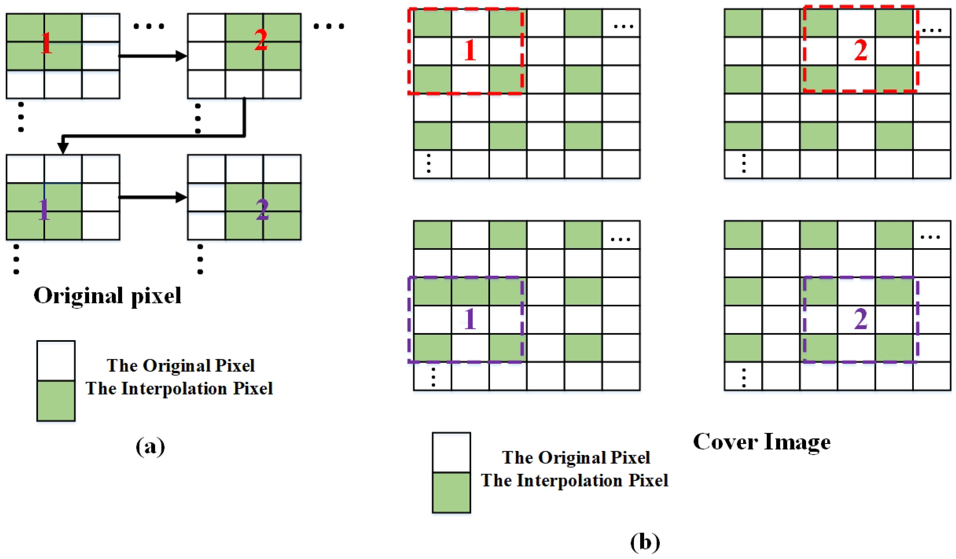
Figure 1. Image segmentation: (a) upsampling; (b) block-based processing.
Electronics 14 03498 g001
Figure 2. Examples of five types of prediction.
Electronics 14 03498 g002
Figure 3. Example of the embedding process.
Electronics 14 03498 g003
Figure 4. Example of the extraction process.
Electronics 14 03498 g004
Figure 5. Four cases of improved methodology.
Electronics 14 03498 g005
Figure 6. Comparison of EC and PSNR for Chi et al.’s [17] method and the proposed method: (a) Lena image, (b) Boat image, (c) Couple image, (d) Airplane image, (e) Baboon image, and (f) Pepper image.
Electronics 14 03498 g006
Figure 7. Comparison in terms of (a) PSNR, (b) SSIM, and (c) EC for the Lena image with Chi et al.’s [17] method.
Electronics 14 03498 g007
Figure 8. Comparison in terms of (a) PSNR, (b) SSIM, and (c) EC for the Airplane image with Chi et al.’s [17] method.
Electronics 14 03498 g008
Figure 9. Comparison of images (a) Lena (b) Baboon (c) Boat (d) Airplane between the proposed scheme and Chi et al. [17] for different embedding capabilities.
Electronics 14 03498 g009
Figure 10. Comparison between the original image (a) and stego-image (b).
Electronics 14 03498 g010
Table 1. The mapping table for embedding data.
Stego value P P 5 P 4 P 3 P 2 P 1 P P + 1 P + 2 P + 3 P + 4
Decimal secret data D9753102468
Table 2. Comparison with different schemes on EC, PSNR, and SSIM.
ImageMetricT = 2T = 3T = 4T = 5T = 2T = 3T = 4T = 5
Chi et al. [17] Proposed Method
LenaEC262,145393,217524,289655,361274,399408,708538,493684,538
PSNR35.9635.4533.9130.4636.2336.1235.1532.51
SSIM0.94030.92520.87200.72230.97840.97650.95810.8512
PeppersEC262,139393,118521,709634,751268,346407,293538,802683,234
PSNR33.9633.6432.5629.9032.6932.6131.2828.01
SSIM0.90380.89030.84230.70980.96470.96180.88240.7656
BaboonEC262,083393,052524,033654,811273,577407,988535,518682,674
PSNR26.4126.3726.1525.3628.4928.5028.3526.80
SSIM0.86480.86000.84260.78310.99360.99280.98980.9779
BoatEC262,145393,217524,177647,081268,687410,362539,779678,808
PSNR32.4032.1831.3629.1432.9732.6331.6529.64
SSIM0.90250.89240.85400.74670.95860.89950.86090.7551
BarbaraEC262,145393,217524,289655,331270,583408,793538,716683,462
PSNR28.2228.1227.7926.6735.2335.1534.2331.30
SSIM0.90330.89280.85530.74700.98350.98240.96760.8549
CoupleEC262,031392,839522,269646,126274,005406,291548,023680,247
PSNR32.5332.2931.4729.2528.4928.5028.3526.80
SSIM0.92370.91400.87900.77470.99360.99280.98980.9779
AirplaneEC262,145393,217524,289655,346270974406149534210686874
PSNR33.3833.1032.1229.5833.6033.5032.5029.89
SSIM0.95670.94020.88160.72490.9640.9470.8510.732
Table 3. Comparison of PSNR with different methods.
Image[18][19][14]Ours
Lena26.8230.1524.2032.51
Peppers25.9928.1324.2028.01
Airplane24.6627.4324.2029.89
Disclaimer/Publisher’s Note: The statements, opinions and data contained in all publications are solely those of the individual author(s) and contributor(s) and not of MDPI and/or the editor(s). MDPI and/or the editor(s) disclaim responsibility for any injury to people or property resulting from any ideas, methods, instructions or products referred to in the content.