Abstract
The highly complex memristive chaotic map provides an excellent alternative for engineering applications. To design a memristive chaotic map with high complexity, this paper proposes a new three-dimensional memristive chaotic map (named MLM) by cascading and coupling a non-locally active memristor with a locally active memristor. The dynamical behaviors of MLM are revealed through phase diagrams, Lyapunov exponent spectra, bifurcation diagrams, and dynamic distribution diagrams. Notably, the internal frequency of MLM exhibits unique LE-controlled behavior and shows an extension of the chaotic parameter range. The high complexity of MLM is validated through the use of Spectral entropy (SE) and C0, and Permutation Entropy (PE) complexity algorithms. Subsequently, a pseudorandom number generator (PRNG) based on MLM is designed. NIST test results validate the high randomness of the PRNG. Finally, the STM32 hardware platform is used to implement MLM, and attractors under different parameters are measured by an oscilloscope, verifying the numerical analysis results.
1. Introduction
The memristor, due to its unique nonlinear characteristics and memory effect, has attracted the attention of many scholars. It is widely applied in fields such as artificial neural networks [1], neural morphology computing [2,3], chaotic circuits [4,5], chaotic systems [6,7], and others. The research on the memristor has a history of several decades, first proposed in 1971 [8]. It became the fourth fundamental electronic component, alongside resistors, inductors, and capacitors, due to its establishment of a relationship between charge and flux. Since then, its theory has been continuously refined by its proposer, Professor Chua [9,10,11]. Another important milestone occurred in 2008, when HP Labs reported the first physically realized memristor, which provided the first validation of the memristor’s feasibility [12]. This breakthrough offered a valuable reference for further research on memristors.
Chaotic systems can be classified into continuous chaotic systems and discrete chaotic systems (i.e., chaotic maps). They exhibit unpredictability and high complexity, characterized by inherent randomness, noise-like behavior, sensitivity to initial conditions, ergodicity, and boundedness [13]. Therefore, chaotic systems are often chosen as a backup option for many applications based on randomness, such as secure communication and data encryption [14,15]. Information security is a fundamental requirement in today’s information age, and the growing demand for security has driven the development of chaotic system research. As a nonlinear system, a chaotic system is composed of nonlinear terms. Therefore, memristors, which possess nonlinear characteristics, have become an excellent option for constructing chaotic systems. It has been proven that memristor-based chaotic systems can exhibit complex dynamic behaviors, with memristors playing a key role in generating complex chaos. Bao et al., by using a memristor to replace the coupling resistor in the realization circuit of a three-dimensional chaotic system with one saddle and two stable node-foci, present a novel memristive hyperchaotic system that exhibits coexisting infinitely many hidden attractors [16]. Zhou et al., by replacing the resistor in a Twin-T network with a generalized flux-controlled memristor, propose a simple fourth-order memristive Twin-T oscillator. By adjusting the parameters, the system can generate various types of chaotic attractors [17]. Ma et al. study a novel and simple chaotic circuit composed of a memristor, a memcapacitor, and a linear inductor connected in parallel. The researchers then establish the dimensionless mathematical model for the circuit and discover 19 different chaotic attractors. Additionally, several special phenomena are observed, such as state transition, chaos degradation, and multiple coexisting attractors [18]. Hu et al. propose a new chaotic system with only one equilibrium point by introducing a smooth quadratic flux-controlled memristor into the VB2 chaotic system. This system features 14 uniquely shaped attractors and exhibits multistable and transient behaviors [19].
Multi-scroll attractors, an important research topic in continuous chaotic systems, have attracted the attention of many researchers [20,21]. Lai et al. propose a new memristor model characteristic using a hyperbolic function series. By integrating different numbers of memristors into a Hopfield neural network (HNN), they create a memristive HNN capable of generating grid-like multiple vortex attractors [22]. Wang et al. study an improved memristive chaotic system with multi-scroll and multi-pinched hysteresis loops through the function design technique. The multi-scroll and multi-pinched hysteresis loops are determined only by the time length. Then, from an application perspective, they propose an adaptive sliding mode synchronization approach for this multi-scroll and multi-pinched hysteresis loops memristive chaotic system, providing an effective approach for the robust design of uncertain systems [23]. The aforementioned research results focus on the study of memristors in continuous systems. Discrete memristors (DM) were only theoretically introduced by He et al. in 2020 [24], and their related theories were refined in 2022 [25]. Therefore, the development time of research on chaotic map of memristors based on DMs is still relatively short.
Compared to continuous chaotic systems, chaotic maps offer several irreplaceable advantages. For instance, continuous systems that exhibit hyperchaotic behavior must be at least four-dimensional [22], while many two-dimensional (2D) chaotic maps can generate chaotic behavior, and even exhibit hyperchaotic behavior [26]. Moreover, due to the differential form of chaotic maps, they align well with the design of digital circuits, making them suitable for applications such as digital image encryption and other related engineering fields; therefore, the study of memristive chaotic map is an important topic [27]. Peng et al. propose a DM model and incorporate it into the Hénon map, designing a memristor-based discrete Hénon map. The new map exhibits a broader chaotic region and greater complexity compared to the original Hénon map. The introduction of the memristor effectively enhances the chaotic characteristics of the Hénon map [28]. Li et al. propose a DM and couple it with four existing 1-dimensional (1D) discrete maps to construct four 2D memristive hyperchaotic maps. These 2D memristive maps exhibit complex dynamic behavior that depends on the memristor’s initial boost and the coupling strength. The analysis results indicate that the DM increases chaotic complexity, and these 2D memristive maps generate hyperchaos [29]. Yuan et al. propose the multi-DM cascading and parallel operation of DM. Additionally, basic cascading and parallel operations can be combined for hybrid operations to construct complex systems. Subsequently, three DMs are presented, and these are combined with the proposed structure to introduce three chaotic maps. Numerical analysis verifies their rich dynamic behavior, providing valuable references for the design of memristive chaotic maps [30]. Wang et al. construct a new 5D hyperchaotic map by adding four DMs, after parallel cascading hybrid operations, to a sine map. Numerical analysis reveals the complex dynamic characteristics of the map and demonstrates its unique super-multistable behavior [31]. Luo et al. propose three memristive chaotic maps, which exhibit hyperchaotic dynamics with high Lyapunov exponent, wide distribution of internal variables, and diverse multi-pulse discharge modes [32]. Lai et al. propose a 4D memristive hyperchaotic map, which exhibits complex dynamic behavior and high unpredictability [33]. Gao et al. introduced a novel discrete chaotic system using dual memristors. Through bifurcation diagrams, Lyapunov exponent spectra, and complexity analysis, it was verified that compared to a single memristor, this system exhibits richer and more complex dynamic behavior [34]. Recently, Bao et al. constructed discrete memristive Hopfield neural networks by using discrete memristors as the variable synaptic weights between neurons [35,36]. By incorporating a memristor with an internal multisegment state function into a two-neuron Hopfield neural network, they developed a novel discrete-time memristive two-neuron HNN (DMT-HNN) capable of generating complex multi-stripe/wave hyperchaos [35].
Additionally, there is a special type of memristor known as the locally active memristor (LAM), which has more complex dynamic characteristics than the non-locally active memristor. In recent years, Ma et al. propose a discrete LAM and introduce it into the existing 2D generalized square map (2D-GSM), resulting in a new three-dimensional chaotic map. Compared to the original system, the new map expands its hyperchaotic region after adding the locally active discrete memristor and is capable of generating more complex behaviors [37]. This proves that the discrete LAM can achieve the generation and enhancement of chaos. Subsequently, Zhao et al. propose a discrete model of the LAM and construct a three-dimensional (3D) memristive multi-well map (LAM-SCM map) by combining the LAM with the existing sine and cosine modulation (SCM) map. Numerical simulations reveal the memristor parameters’ dependence on the lossless displacement and self-shift of the multi-cavity attractor, as well as the initial boosting behavior, which characterizes the performance enhancement of the LAM on the existing SCM map [38].
However, current research on chaotic maps based on discrete active memristors remains limited and requires further advancement. Therefore, we propose a novel memristive map based on both non-locally active memristors and LAM, revealing its complex dynamic behaviors. The novelty and contributions of this work are summarized as follows:
(1) A 3-dimensional memristive chaotic map based on the coupling of non-locally active and locally active memristors is proposed for the first time.
(2) Internal frequency parameters are embedded within the trigonometric functions. The embedded parameters exhibit control over the chaotic map’s LEs and can also extend the map’s chaotic parameter range and enhance its complexity.
The rest of the paper is organized as follows: Section 2 introduces a LAM and a non-locally active memristor, and proposes a novel memristive chaotic map. Section 3 investigates the dynamical behavior of the proposed chaotic map, followed by an analysis of the map’s complexity. Section 4 designs an application for generating pseudo-random sequences based on the proposed map and verifies the practical feasibility of the discrete memristive chaotic map using the STM32 platform.
2. MLM Discrete Map
2.1. Cosine Memristor
According to Chua’s definition of a memristor, and the discretization method of continuous memristors [11], the mathematical model of an ideal charge-controlled discrete memristor is represented as follows [24]:
where q(t) represents the charge, M(q) represents the memristance, i(t) represents the bipolar periodic input current, and v(t) represents response voltage.
Cosine discrete memristor is commonly used to construct chaotic maps in discrete memristors, showcasing remarkable chaotic behavior. Its model is as follows:
According to the cosine modulation method proposed in the recent literature, the modulated cosine memristor (MCM) is as follows:
To verify the memristor fingerprints of the modulated memristor, a bipolar periodic signal in = A∙sin(ω∙n) is selected as the input. By varying the frequency and amplitude of the input signal, Figure 1 shows the memristor output signals as pinched hysteresis loops. Figure 1a presents the output curve of the memristor at different input frequencies when the input amplitude is 1.5; Figure 1b shows the response curve of the memristor at different input amplitudes when ω = 0.2 rad/s. It can be seen in Figure 1a, during the process of adjusting ω from 0.2 rad/s to 0.5 and finally to 3 rad/s, the side lobe area of the memristor’s output curve continuously decreases. When ω reaches 3 rad/s, the output of the memristor becomes a single-valued function of the input’s zero-crossing point. By changing the input amplitude A, Figure 1b shows the pinched hysteresis loops of the memristor with amplitudes adjusted to 0.5, 1, and 2 with A = 1.5, respectively. The above results verify the memristor fingerprints of the modulated memristor.
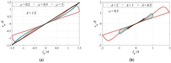
Figure 1.
The pinched hysteresis loops for MCM when applying the excitation current in = A∙sin(ωn): (a) for different ω (ω = 0.2, 0.5, or 3 rad/s) at A = 1.5; (b) for different A (A = 0.5, 1, or 2) at ω = rad/s.
2.2. Locally Active Discrete Memristor
According to the literature, the mathematical model of the bistable locally active discrete memristor (LADM) is as follows [39]:
In the above mathematical model, in represents the input signal applied to the memristor, vn represents the output signal of the memristor, qn represents the charge, and M(qn) represents the memristance. The parameters a, b, and c represent the memristor parameters. In the following discussion, a, b, and c will be fixed as 0.1, 1.1, and −0.1, respectively.
Similarly to the cosine memristor described above, a bipolar periodic signal in = A∙sin(ω∙n) is selected as the input signal for the LADM to test its memristor fingerprints. The output response of the LADM at different frequencies or amplitudes of the input signal is shown in Figure 2. In Figure 2a, the fingerprints of the memristor’s pinched hysteresis loops, where the side lobes passing through the origin progressively shrink into a single-valued function as the input signal frequency increases, is shown. In Figure 2a, the characteristic of the sidelobes of the hysteresis loop passing through the origin continuously contracting to a single valued function as the input signal frequency increases is demonstrated. By modulating the amplitude of the input signal, Figure 2b shows the pinched hysteresis loops with a ‘8’ shape at the zero-crossing point, when the input amplitudes are 0.5, 1, and 2 with ω = 0.5. These test results indicate that the LADM satisfies the definition of a memristor [11].
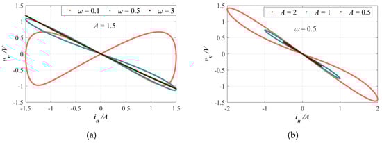
Figure 2.
The pinched hysteresis loops for LADM when applying the excitation current in = A∙sin(ωn): (a) for different ω (ω = 0.1, 0.5, or 3 rad/s) at A = 1.5; (b) for different A (A = 0.5, 1, or 2) at ω = 0.5 rad/s.
After determining the basic memristor fingerprints of the LADM, its non-volatile property is also an important characteristic [38]. According to the analysis method proposed in the literature [11], we can use the power-off plot (POP) to analyze the non-volatile of the memristor. It describes the relationship between qn+1 − qn and qn when in = 0. Therefore, the following equilibrium equation can be obtained:
When the curve in the power-off plot (POP) intersects the qn axis at two or more points with a negative slope, the memristor exhibits non-volatile characteristics [11]. The POP of the memristor are shown in Figure 3a. It can be observed that the power-off curve intersects the qn axis at three points, indicating three equilibrium points for the memristor. Among these, E2 is the equilibrium point with a positive slope, meaning it is unstable, while E1 and E3 are equilibrium points with a negative slope, indicating that they are asymptotically stable. When the input current (in) of the memristor is zero, the memristor will converge to one of the asymptotic equilibrium points, E1 (when q0 < 0) or E3 (when q0 > 0). As shown in the asymptotically stable memory plot (Figure 3b), the curve eventually converges to −1 or 1 as the number of iterations increases. The existence of E1 and E3 confirms the non-volatile characteristics of the memristor.
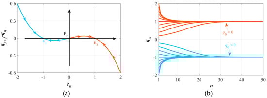
Figure 3.
Non-volatile verification: (a) POP curve; (b) Asymptotically stable memory plot.
The locally active characteristics of the LADM can be detected through its DC I–V plot. If there is a region with a negative slope in the DC I–V plot, the memristor can be classified as a locally active memristor. Therefore, by setting qn+1 − qn = 0, vn = V, and combining with Equation (4), we can derive
where I is the DC current, V is the DC voltage, and q is the internal state variable of the memristor.
When q continuously varies from −2 to 2, the DC I–V characteristics of the memristor are plotted in Figure 4. It can be clearly observed that the memristor exhibits two negative slope regions (blue and red), as well as two locally active regions. Therefore, the LADM can be classified as a locally active memristor.
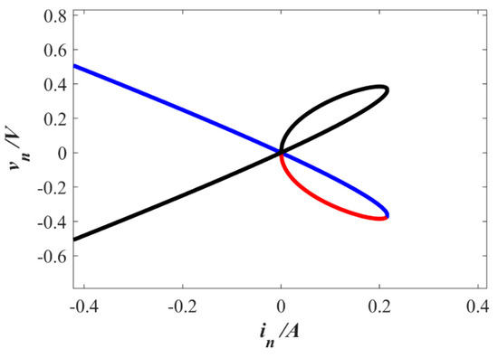
Figure 4.
DC I–V plot of LADM.
2.3. MLM Model
A novel three-dimensional memristive chaotic map (named MLM) is proposed by cascading the MCM behind the LADM and parallel coupling the two memristors with a sine nonlinear term. The structural diagram is shown in Figure 5.
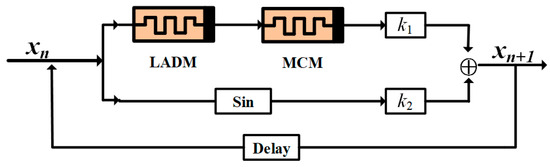
Figure 5.
The structure diagram of MLM.
Therefore, the mathematical model of the proposed memristive chaotic map is expressed as follows:
where k1 and k2 are coupling parameters, d1 and d2 are the internal frequency parameters, which will serve as the control parameters for the memristive chaotic map.
2.4. Analysis of Fixed Points
The fixed point (x*, y*, z*) of the MLM can be obtained by solving the following equation:
Through Equation (8), we can conclude that when x = 0, the three fixed points of the MLM are (x, y, z) = (0, 0, 0), (x, y, z) = (0, 1, 0), and (x, y, z) = (0, −1, 0). The stability of these fixed points can be determined by the Jacobian matrix. Therefore, the Jacobian matrix of the map is as follows:
where j11 = k1∙tanh(y)∙cos(d2∙z) + k2∙d1∙cos(d1∙x), j12 = k1∙x∙cos(d2∙z)∙(1 − (tanh(y))2), j13 = − d2∙k1∙x∙tanh(y)∙sin(d2∙z), j31 = cos(z + x∙tanh(y))∙tanh(y), j32 = x∙cos(z + x∙tanh(y))∙(1 − (tanh(y))2), j33 = cos(z + x∙tanh(y)). Therefore, we can obtain the Jacobian matrix for the fixed point (0, 0, 0):
It can be concluded that λ1 = k2∙d1, λ2 = b, λ3 = 1. The map is stable only when all the eigenvalues are inside the unit circle. Therefore, the stability of the map depends on whether |λ1| or |λ2| is greater than 1. When |λ1| and |λ2|are both less than or equal to 1, the map is stable. When |λ1| or |λ2| is greater than 1, the map is unstable. Therefore, the stability of the map depends on k2, d1, and b.
For (0, 1, 0) and (0, −1, 0), by using their Jacobian matrices, we can obtain the eigenvalues for (0, 1, 0) as {λ1 = k1∙tanh(1) + 1, λ2 = −3a + b, λ3 = 1}, and for (0, −1, 0) as {λ1 = k1∙tanh(−1) + 1, λ2 = −3a + b, λ3 = 1}. It can be seen that in this case, the stability of the map depends on k1, a, and b.
3. Dynamics Analysis
In this section, various numerical methods and evaluation metrics are employed to analyze the complex dynamical behaviors of the MLM, including Lyapunov exponent spectra, bifurcation diagrams, phase diagrams, and dynamic distribution maps. The Lyapunov exponents (LE) are calculated using Wolf’s Jacobi algorithm [40]. Additionally, the complexity of the MLM is analyzed using Spectral Entropy (SE), C0, and Permutation Entropy (PE) complexity algorithms.
3.1. Parameters Relied Dynamics
The bifurcation process and Lyapunov exponent spectrum controlled by a single parameter have greatly facilitated the in-depth understanding of the attractor evolution mechanism. They provide us with a direct visual window to help reveal the evolution processes of state evolution in chaotic systems. The Lyapunov exponent (LE) quantifies the sensitivity to initial conditions and the unpredictability in chaotic systems. Therefore, the coupling parameters (k1, k2) and internal frequency parameters (d1, d2) are used as control parameters, with the initial conditions (IC) (x0, y0, z0) set to (1, 1, 1).
3.1.1. Coupling Parameters Relied Dynamics
With (k2, d1, d2) = (4, 1, 1), the dynamic evolution of the system as k1 varies from −1.4 to 1.4 is shown in Figure 6a. It can be observed that the dynamic evolution for k1 ∈ [−1.4, 0) is almost symmetric with respect to the y-axis compared to k1 ∈ (0, 1.4). Therefore, analyzing the system for k1 ∈ (0, 1.4] provides insight into the evolution process across the entire range. When k1 ∈ (0, 1), the majority of cases exhibit LE1 > 0, indicating that the system is primarily in a chaotic state within this range. Additionally, in this range, there are a few instances where LE1 ≤ 0, indicating the appearance of rare periodic windows. For k1 ∈ (1, 1.067) and k1 ∈ (1.195, 1.292), the system is in a periodic state, while for k1 ∈ (1.067, 1.195) and k1 ∈ (1.292, 1.4), the system remains in a chaotic state.
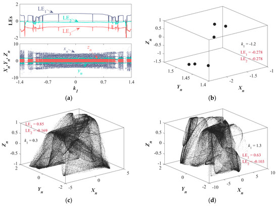
Figure 6.
Set IC = (1, 1, 1), LE spectrums, bifurcation diagrams, and phase diagrams: (a) LE spectrums and bifurcation diagrams of {k1 ∈ [−1.4, 0], (k2, d1, d2) = (4, 1, 1)}; (b–d) phase diagrams of k1 = 1.2, k1 = 0.3, and k1 = 1.3.
As k1 changes, the system evolves attractors with different topological structures. Figure 6b–d show the period-6 attractor (k1 = −1.2) and two types of chaotic attractors (k1 = 0.85 and k1 = 1.3).
With (k1, d1, d2) = (1,1,1), the LEs spectrum and corresponding bifurcation diagram for k2 ∈ [0, 6] are shown in Figure 7a. For k2 ∈ (0, 2.63), the map exhibits a periodic state with a period of 1. As k2 continues to increase, in the interval k2 ∈ (2.63, 2.84) the system evolves into a quasi-periodic attractor with a maximum LE of 0, as shown in Figure 7b for the quasi-periodic attractor at k2 = 2.83. In the interval (2.84, 4), the system continuously shifts between periodic and chaotic states, with the periodic attractor of period-11 at k2 = 2.9 shown in Figure 7c. When k2 extends further to (4, 6), the chaotic state occupies the majority of the parameter space, with a few periodic windows emerging. The chaotic attractor at k2 = 5.5 is shown in Figure 7d.
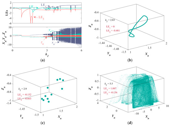
Figure 7.
Set IC = (1, 1, 1), LE spectrums, bifurcation diagrams, and phase diagrams: (a) LE spectrums and bifurcation diagrams of {k2 ∈ [0, 6], (k1, d1, d2) = (1, 1, 1)}; (b–d) phase diagrams of k2 = 2.83, k2 = 2.9, and k2 = 5.5.
3.1.2. Internal Frequencies Relied Dynamics
In this subsection, the internal frequencies d1 and d2 are analyzed as controllable variables to reveal the dynamic evolution of the map, with (k1, k2) fixed at (1, 4). The LEs spectrum and bifurcation diagrams for d1 ∈ [1, 20] are presented in Figure 8a. Overall, LE1 of the map shows a gradual increase, while LE2 and LE3 remain largely unchanged and both are less than 0. In more detail, when d1 is relatively small, i.e., d1 ∈ [1, 3.59], periodic windows appear as d1 changes. As d1 continues to evolve, the attractors of the map also undergo continuous evolution, as shown in Figure 8c,d for the three chaotic attractors at d1 = 2, d1 = 4, and d1 = 20.
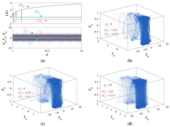
Figure 8.
Set IC = (1, 1, 1), LE spectrums, bifurcation diagrams, and phase diagrams: (a) LE spectrums and bifurcation diagrams of {d1 ∈ [1, 20], (k1, k2, d2) = (1, 4, 1)}; (b–d) phase diagrams of d1 = 2, d1 = 4, and d1 = 20.
By comparing the internal frequency d1, the map exhibits different behaviors when d2 changes. As seen in Figure 9a, overall, LE1 of the map also shows a gradual increase. The difference is that LE2 and LE3 also show an upward trend. When d2 rises to 4.23, LE2 becomes positive, and LE2 continues to increase as d2 increases. At this point, the map exhibits two positive LEs, indicating the emergence of hyperchaos. The map exhibits chaotic characteristics in two dimensions. A hyperchaotic attractor (at d2 = 20) is shown in Figure 9d, while chaotic attractors at d2 = 2 and d2 = 4 are shown in Figure 9b and Figure 9c, respectively.
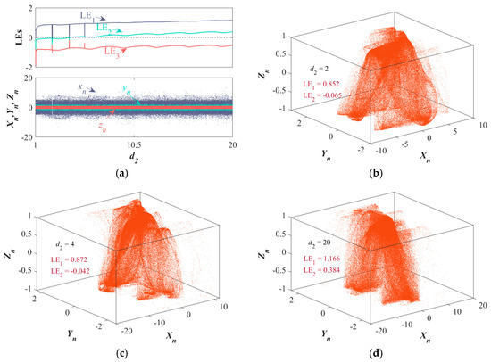
Figure 9.
Set IC = (1, 1, 1), LE spectrums, bifurcation diagrams, and phase diagrams: (a) LE spectrums and bifurcation diagrams of {d2 ∈ [1, 20], (k1, k2, d1) = (1, 4, 1)}; (b–d) phase diagrams of d2 = 2, d2 = 4, and d2 = 20.
To further reveal the effects of internal frequencies d1 and d2 on the map, their research range has been expanded. Setting d2 = 1 and d1 ∈ [1, 1010], the LE spectrum and bifurcation diagram are shown in Figure 10a. It can be seen that the bifurcation diagram remains generally stable. LE1 increases continuously as log10(d1) grows, and visually, it is apparent that LE1 forms a straight line, revealing a linear relationship between LE1 and log10(d1), meaning LE1 and 10d1 exhibit a linear correlation. The phenomenon of LE2 and LE3 is consistent with that in Figure 8a, where they remain nearly constant and less than or equal to 0. When setting d1 = 1, the analysis range for d2 is expanded to [1, 1015], and Figure 10b shows the dynamic evolution of the map as d2 ∈ [1, 1015]. Meanwhile, the bifurcation diagram also remains stable overall. As d2 increases, both LE1 and LE2 gradually rise, eventually coinciding. Within the range d2 ∈ [105, 1015], LE1 and LE2 with d2 exhibit an approximately linear relationship, while LE3 remains around 0. Therefore, the parameter d1 controls LE1, and d2 controls both LE1 and LE2.
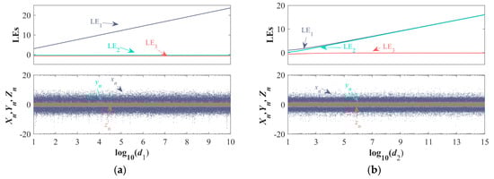
Figure 10.
Set IC = (1, 1, 1), LE spectrums and bifurcation diagrams: (a) for d1 ∈ [1, 1010] and (k1, k2, d2) = (1, 4, 1); (b) for d2 ∈ [1, 1015] and (k1, k2, d1) = (1, 4, 1).
According to Figure 10a, when log10(d1) = 1, LE1 = 2.995, and when log10(d1) = 10, LE1 = 23.72. Therefore, we can deduce the approximate relationship between LE1 and d1. For d1 ∈ [1, 1010], with IC = (1, 1, 1) and (k1, k2, d2) = (1, 4, 1), the relationship is as follows:
According to Figure 10b, when log10(d2) = 5, (LE1, LE2) = (4.692, 4.436), and when log10(d2) = 15, (LE1, LE2) = (16.11, 16.04). Therefore, for d2 ∈ [105, 1015], with IC = (1, 1, 1) and (k1, k2, d1) = (1, 4, 1), the approximate relationship between (LE1, LE2) and d2 is as follows:
By using Equations (8) and (9), we can effectively control the system’s LEs, providing us with a convenient control method.
3.2. Complexity Analysis
Complexity analysis plays a crucial role in assessing the similarity between chaotic sequences and ideal random sequences, making it an essential tool for the dynamical characterization of chaotic systems [41]. There is a positive correlation between the complexity of chaotic sequences and their closeness to ideal random sequences: the higher the complexity, the closer the chaotic sequence is to an ideal random sequence. Complexity analysis can be divided into behavioral complexity and structural complexity, offering two fundamental perspectives for studying chaotic systems. Structural complexity algorithms are commonly used in dynamic analysis, where they evaluate the complexity of sequences by examining their frequency and energy spectrum characteristics within the transformation domain.
3.2.1. Spectral Entropy Complexity Analysis
The study of system complexity provides crucial theoretical guidance for the application of chaotic systems in various fields, including cryptographic communication. Spectral entropy (SE) in structural complexity algorithms is used to analyze the complexity of MLM, with the SE calculated by applying a Fourier transform in combination with Shannon entropy with its range being [0, 1]. To better reflect the energy information of the signal, the sequence L(n) for the chaotic sequence {x(n), n = 0, 1, 2, 3, …, N − 1}, generated by a chaotic system of length n, is obtained through the following equation:
Subsequently, perform a discrete Fourier transform (DFT) on X (n) to obtain M (n)
where k = 0, 1, …, N − 1. By taking the first half of the sequence for calculation, the relative power spectrum of the transformed sequence M(k) is computed. According to Parseval theorem, the power spectrum value at a certain frequency point is determined by the following equation:
where i is an integer i ∈ [0, N/2 − 1]. The total power of the sequence can be obtained from Equation (13):
The probability of the relative power spectrum of the sequence is calculated as follows:
From the relationship between S(i) and Stotal, it is known that (p0 + ⋯ + pN/2−1) = 1. By combining this with Shannon entropy methods, the SE can be obtained from Equation (15):
To facilitate comparative analysis, the SE is normalized. The formula for the normalized SE is shown in Equation (16) [42]:
The SE distribution on the two-dimensional plane (k2 − k1), with fixed values of (d1, d2) as (1, 1) and {k1 ∈ [−1.4, 1.4], k2 ∈ [0, 6]}, is shown in Figure 11a. In this diagram, darker colors represent higher SE values, while the white areas indicate that the map is in a divergent state. It can be observed that, within the given parameter range, the SE is greater than 0.9 in most of the area, with the maximum value around 0.9503.

Figure 11.
Set (d1, d2) = (1, 1) and {k1 ∈ [−1.4, 1.4], k2 ∈ [0, 6]}: (a) the SE complexity distribution diagrams; (b) the dynamic distribution diagram.
Furthermore, to further reveal the SE distribution, a dynamic distribution diagram representing the map’s dynamic behaviors is plotted in Figure 11b. Different color blocks represent various dynamic behaviors, specifically: dark blue, green, purple, dark red, dark cyan, blue, yellow, and orange correspond to the single-period (SP), period-2 (P2), period-4 (P4), period-8 (P8), multi-period (MP), quasi-periodic (QP), chaotic (CH), and hyper-chaotic (HCH) attractors, respectively. The black areas indicate the divergent state of the map, which corresponds to the white areas in Figure 11a. By comparing Figure 11a,b, it can be observed that when the map is in a chaotic state, it exhibits high SE, while the SE corresponding to its periodic states is relatively low.
3.2.2. C0 Complexity Analysis
To further validate the high complexity of the map, its C0 complexity is analyzed. The C0 complexity is also based on the discrete Fourier transform, but it reflects the proportion of irregularities in the sequence, with a range of [0, 1]. The higher the proportion of irregular components in the sequence’s energy, the more its signal characteristics approach those of a random sequence, thereby reflecting the system’s complexity.
The steps for calculating the measured value are as follows.
For the chaotic sequence {x(n), n = 0, 1, 2, 3, …, N − 1}, perform a discrete Fourier transform (DFT) on x(n) to obtain F(k)
where k is an integer k ∈ [0, N − 1]. Subsequently, the mean square value of F(k) is calculated using the following equation:
Let
where r(r > 0) is the control parameter. The inverse Fourier transform of M(k), denoted as m(k), is obtained from Equation (20)
where n = 0, 1, 2, …, N − 1. Finally, the C0 algorithm’s complexity calculation is defined as in Equation (21).
The C0 complexity for the two-dimensional parameters {k1 ∈ [−1.4, 1.4], k2 ∈ [0, 6]} is plotted in Figure 12. It can be seen that Figure 12 corresponds with Figure 11a,b, and the C0 complexity of the map is 0.9933.
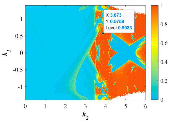
Figure 12.
Set (d1, d2) = (1, 1) and {k1 ∈ [−1.4, 1.4], k2 ∈ [0, 6]}, the C0 complexity distribution diagram.
3.2.3. Permutation Entropy Complexity Analysis
Permutation Entropy (PE) is an important tool used to assess the complexity of time series. It quantifies the dynamic characteristics of a sequence by analyzing the arrangement patterns of data points within the sequence. By performing combinatorial analysis on the time series, permutation entropy can quantitatively describe the complexity of the sequence, i.e., its uncertainty or degree of disorder. A higher permutation entropy value typically indicates that the system’s behavior is more complex and difficult to predict, while a lower permutation entropy value may suggest that the system’s behavior is more regular and predictable. The calculation process is as follows:
First, for the chaotic sequence of length N, {x(n), n = 0, 1, 2, 3, …, N − 1}, phase space reconstruction is performed, yielding:
where m is the embedding dimension, τ is the delay time, and k is the number of X. The number of elements in each X is m.
Then, the elements of Xi are sorted in ascending order to obtain the sorted array Y = [j1, …, jm], i = 1, 2, …, k. Taking Xi with m = 4 as an example, if Y = [3, 1, 4, 2], it represents
In addition, if there are equal elements in Xi, they are sorted according to their original order in the sequence. For each X, we can obtain a sequence Sl = [j1, …, jm], where l = 1, 2, …, k and k ≤ m!. Subsequently, we can calculate the permutation entropy HP:
where Pj is the probability of the occurrence of the symbol sequence, and the maximum value of HP is ln(m!). To facilitate comparison and analysis, HP is normalized, as shown in Equation (25).
The PE distribution for the two-dimensional parameters {k1 ∈ [−1.4, 1.4], k2 ∈ [0, 6]} is plotted in Figure 13. It can be seen that Figure 13 corresponds with Figure 11a,b and Figure 12. The process of the spectral color gradually transitioning from dark blue to light yellow corresponds to an increasing PE.
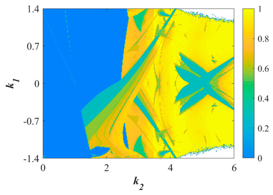
Figure 13.
Set (d1, d2) = (1, 1) and {k1 ∈ [−1.4, 1.4], k2 ∈ [0, 6]}, the PE distribution diagram.
Overall, the analysis of SE, C0, and PE complexity confirms the high complexity of the map. This indicates that the map exhibits high complexity, and the chaotic sequences it generates possess strong security features
3.2.4. The Impact of Internal Frequencies on Complexity Distribution
The internal frequencies d1 and d2 have the ability to regulate the dynamics of the map. To analyze their impact on the dynamical behavior and complexity of the map, the dynamic distribution map, SE, C0, and PE complexity distribution for {k1 ∈ [−1.4, 1.4], k2 ∈ [0, 6]} are plotted in Figure 14, where Figure 14(a1–a4) correspond to (d1 = 104, d2 = 1) and Figure 14(b1–b4) correspond to (d1 = 1, d2 = 104).
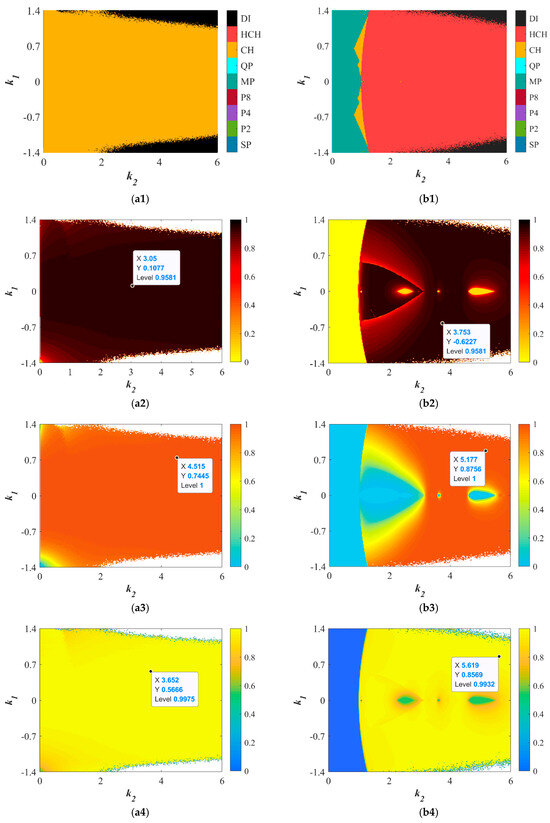
Figure 14.
Set {k1 ∈ [−1.4, 1.4], k2 ∈ [0, 6]}: (a1) the dynamic distribution diagram of (d1, d2) = (1, 104); (a2) the SE complexity distribution diagrams of (d1, d2) = (1, 104); (a3) the C0 complexity distribution diagrams of (d1, d2) = (1, 104); (a4) the PE distribution diagrams of (d1, d2) = (1, 104); (b1) the dynamic distribution diagram of (d1, d2) = (104, 1); (b2) the SE complexity distribution diagrams of (d1, d2) = (104, 1); (b3) the C0 complexity distribution diagrams of (d1, d2) = (104, 1); (b4) the PE distribution diagrams of (d1, d2) = (104, 1).
When (d1 = 104, d2 = 1), the map only exhibits chaotic and divergent behaviors across the entire parameter range. Almost the entire chaotic region has an SE, C0, and PE complexity above 0.95, with the maximum values reaching 0.9581 for SE, 1 for C0 complexity, and 0.999 for PE. As shown in Figure 14(b1), when (d1 = 1, d2 = 104), the entire parameter range consists of multi-periodic, chaotic, hyper-chaotic, and divergent behaviors, with hyper-chaos occupying most of the range. The SE, C0, and PE complexity in the hyper-chaotic region are generally higher than in the multi-periodic and chaotic areas.
Overall, the internal frequencies d1 and d2 can enhance the chaotic parameter range of the system and increase its complexity.
To highlight the advantages of MLM, it is crucial to compare it with other target maps. To this end, the discrete maps from references [29,34,39,41,42] are selected as comparison objects, the parameters and initial values of MLM are set to (k1, k2, d1, d2) = (1, 4, 1, 1015), IC = (1, 1, 1). Table 1 summarizes the comparison results between MLM and other maps. The comparison items include LE, SE, and C0. It can be seen that key metrics such as LE and SE for MLM are significantly higher than those of other maps, demonstrating the superiority of MLM.

Table 1.
Comparison of (LEs, SE, C0, PE) between different maps.
4. Application in PRNG
4.1. Pseudo-Random Numbers Generator
Pseudorandom number generator (PRNG) is widely used in various fields, such as Monte Carlo simulations [45,46], encryption algorithms [47], and machine learning [48]. Due to the chaotic nature of chaotic systems, they exhibit a high degree of compatibility with PRNGs. Considering that MLM can generate complex dynamic behaviors, particularly hyperchaotic attractors, a MLM-PRNG has been designed.
Two sets of parameters for the MLM are used as the test for the PRNG. They are: {(k1, k2, d1, d2) = (1, 4, 1, 1), IC = (1, 1, 1)} and {(k1, k2, d1, d2) = (1, 5, 100, 1), IC = (1, 1, 1)}. When (k1, k2, d1, d2) is set to (1, 4, 1, 1) and (1, 5, 100, 1), two chaotic sequences of length n are generated, denoted as X(k1, k2, d1, d2)=(1, 4, 1, 1) = {x(1), x(2), ⋯, x(n), ⋯} and X(k1, k2, d1, d2)=(1, 5, 100, 1) = {x(1), x(2), ⋯, x(n), ⋯}. Then, each element of XK is converted into a 52-bit binary number G(n) using the IEEE 754 floating-point standard. The converted set of G(n) forms a binary sequence. Next, the digits from position 35 to 42 in the binary sequence are used as the PRN, which can be represented by Equation (26).
In practical applications, considering the limitations of hardware resources, the computation speed of PRNG algorithms is a crucial factor to consider. Therefore, the execution speed of MLM-based PRNG was analyzed. We conducted performance tests using Matlab 2018b on a PC, with the following steps: (1) select 10 different keys to generate 10 hyper-chaotic sequences of length A, and generate pseudo-random numbers based on these sequences; (2) record the time required to generate each pseudo-random number; (3) calculate the average generation speed of the 10 sets of pseudo-random numbers. The test results show that when A = 106, the execution time of the PRNG is 0.378 s. When A = 107, the execution time is 3.4 s, and when A = 2 × 10⁷, the execution time is 6.77 s.
4.2. NIST SP800-22 Test
The high randomness of the pseudorandom numbers (PRNs) generated by the PRNG is a prerequisite for its application in engineering. Therefore, the National Institute of Standards and Technology (NIST) SP800-22 is selected to test and analyze the randomness of the generated PRNs [49]. NIST SP800-22 is a comprehensive and rigorous testing standard, consisting of 15 subtests. Each subtest outputs a p-value to determine whether the sequence passes the subtest. In NIST SP800-22, statistical error is measured by using a significance level α as the standard for evaluating p-values. According to the recommendations in Ref. [49], α is set to 0.01. In our experiment, the randomness of 120 binary sequences, each of length 106, is chosen as the test subject. Each subtest of the 15 subtests generates a p-value for each binary sequence in the test set. Therefore, 120 p-values are generated in each subtest. When the p-value output by the subtest is greater than α, it is considered that the binary sequence has passed the subtest. The ratio of the sequences that pass a subtest to the total test sequences is called the pass rate the subtest, which is a key indicator of the randomness of the binary sequences. When the significance level α and the number of binary sequences is 120, the minimum pass rate is 0.9628. In addition to the pass rate, another key indicator is p-valueT, which, together with the pass rate, characterizes whether the PRN has high randomness. The process for calculating p-valueT is as follows: first, the interval [0, 1] is divided into ten equal subintervals. Then, the number of p-values within each subinterval is calculated. Finally, a χ2 test is applied to the distribution of the p-values to obtain p-valueT. When p-valueT is greater than 0.0001, it indicates that the sequence has passed the subtest.
Table 2 lists the test results of the random numbers generated by the PRNG in the NIST SP800-22 test. It can be seen that, under both sets of parameters, the pass rate and p-valueT of the PRNs generated by the PRNG are both greater than 0.9628 and 0.0001, respectively. This indicates that the designed PRNG is capable of generating PRNs with high randomness.
Table 2.
The NIST SP800-22 test results of the proposed PRNG with (k1, k2, d1, d2) = (1, 4, 1, 1) or (1, 5, 100, 1), and IC = (1, 1, 1).
4.3. Information Entropy
Information entropy (IE) is an important numerical analysis method for measuring the robustness of the PRNs generated by the PRNG. A larger IE indicates that the PRN has strong robustness, while a smaller IE suggests weak randomness and predictability. Therefore, IE is selected to test the robustness of the PRNs generated by the designed PRNG, and its calculation method is as follows:
where N is the number of bits in each element of the PRN (N = 8), and p(PRNsi) is the probability of each PRNsi. The ideal value of H(PRNs) is N. In our testing. We selected 10 sets of PRNs with random keys as the test objects, and the average value of these 10 sets of test results is 7.975444829495733. The tested value is very close to the theoretical value of N (=8), which verifies the robustness of the PRNs.
4.4. Autocorrelation Analysis
The autocorrelation analysis of the PRNs reflects whether the sequence exhibits repeating patterns, periodicity, or correlation. The formula for calculating autocorrelation is as follows:
where AC refers to the correlation between the sequence signal As and the signal B offset k positions from A, and its range is between [−1, 1]. As is the number of matches between the original sequence and the shifted sequence, and D is the number of mismatches. An AC value close to 1 indicates that most of the bits are the same. When AC is close to −1, it indicates that most of the bits are opposite [50]. An AC value closer to 0 means that the number of same and opposite bits is equal. In this test, a PRN sequence with a length of 240,000 bits was used as the test object. The parameters are set as (k1, k4, d1, d2) = (1, 4, 1, 1), IC = (1, 1, z0), where z0 is a controllable variable. To simultaneously verify the randomness of the PRNs and test the robustness of the PRNG’s chaotic characteristics under different IC, z0 is assigned five different random values. The test results are shown in Figure 15, where the AC values of all five groups of PRNs are very close to 0. This validates the high randomness of the PRNs as well as the robustness of the PRNG.
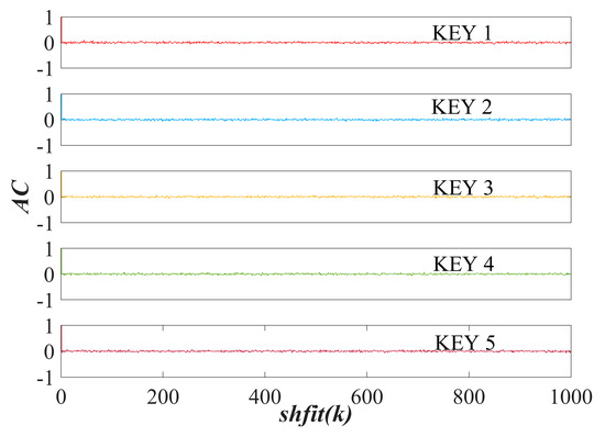
Figure 15.
Autocorrelation analysis under the five secret keys when parameters and IC are set as a (k1, k4, d1, d2) = (1, 4, 1, 1), IC = (1, 1, z0), where z0 = KEY 1, z0 = KEY 2, z0 = KEY 3, z0 = KEY 4, or z0 = KEY 5.
5. Hardware Implementation
The digital hardware platform is an excellent alternative for implementing memristor-based chaotic maps, as its internal computational processes naturally align with the iterative operations of chaotic maps. Therefore, the STM32F103 microcontroller is selected to realize MLM and validate the real-world feasibility of MLM. First, we need to encode the mathematical model of the MLM and its corresponding parameters. The program is then loaded into the microcontroller via J-Link for online debugging. Finally, the generated chaotic signals are transmitted through the DAC8552 to the UNI-T UTD2102CM digital oscilloscope. The DAC8552 is a 16-bit Digital-to-Analog Converter, and it has a resolution of 16 bits, meaning it can represent 216 = 65,536 different discrete output levels. In the experiment, the output range of the DAC8552 is −5 V to +5 V. According to the formula: Least Significant Bit(LBS) = (Vmax − Vmin)/65,535 ≈ ±152.6 μV, therefore the quantization error of the DAC8552 is LBS/2 = ±76.3 μV. In addition, the sampling frequency of the DAC8552 is typically determined by the microcontroller controlling it, with a maximum value of 1 MSPS. Therefore, the sampling frequency of the DAC8552 is set to 1 MSPS.
The minimum system board with microcontroller STM32F103C8T6, analog-to-digital converter DAC8552, and related peripheral interface circuits constitute the required experimental digital hardware platform, as shown in Figure 16.
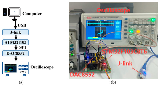
Figure 16.
Circuit experiment: (a) Overall hardware flowchart; (b) actual hardware facilities.
To verify the feasibility of the chaotic map, three sets of parameters {(k1, k2, d1, d2) = (0.6, 3.4, 1, 1), (k1, k2, d1, d2) = (0.7, 3.2,1, 1), (k1, k2, d1, d2) = (0.8, 3.4, 1, 1)} were used to obtain attractors in the x–y plane, which serve as references. The numerical simulation attractors are shown in Figure 17a–c. The attractors generated by the STM32 are presented in Figure 17d–f, and they exhibit a high degree of consistency with the results from the numerical simulation platform shown in Figure 17a–c. This demonstrates the feasibility of the hardware implementation and provides potential applications for the MLM in practical engineering.
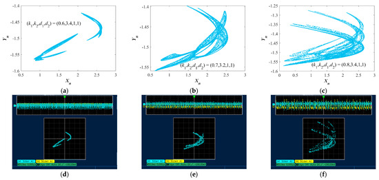
Figure 17.
Three chaotic attractors of three sets of parameters {(k1, k2, d1, d2) = (0.6, 3.4, 1, 1), (k1, k2, d1, d2) = (0.7, 3.2, 1, 1), (k1, k2, d1, d2) = (0.8, 3.4, 1, 1)}: (a–c) numerical simulation results; (d–f) hardware experiment results.
6. Conclusions
This paper proposes a novel three-dimensional memristive chaotic map (named MLM) by sine-modulating a cosine discrete memristor, cascading it with a locally active memristor, and coupling them with a sine nonlinear term. For the first time, non-locally active and locally active memristors are coupled to construct the chaotic map. The dynamical behaviors dependent on the parameters are analyzed through phase diagrams, Lyapunov exponent spectra, bifurcation diagrams, and dynamic distribution maps. Two internal frequencies of this map exhibit distinct control behaviors: d1 controls LE1, while d2 controls both LE1 and LE2. The control trend shows that as the internal frequencies increase, the system’s Lyapunov exponents (LEs) also rise. Concurrently, as d1 and d2 increase, the chaotic parameter range expands, and the periodic window contracts, providing an effective way to control the map’s performance. In practical encryption applications, the expansion of the chaotic range allows the MLM-based encryption system to have a broader parameter space, while the strong chaotic characteristics provide guarantees for the encryption performance of the encryption system. The high complexity of the map is confirmed through SE, C0, and PE algorithms. A pseudorandom number generator (PRNG) based on MLM is then designed, and NIST tests confirm its high randomness. Finally, the map is implemented on the STM32 hardware platform, and attractors captured by the oscilloscope validate the numerical analysis results.
Author Contributions
H.S. and Q.W. conceived and carried out the project. H.S. wrote the manuscript. K.L. Whole analysis and reviewing. K.L. and Y.C. supervising and reviewing. Z.Y.: Manuscript revision. All authors have read and agreed to the published version of the manuscript.
Funding
This work is supported by the Guizhou Provincial Basic Research Program (Natural Science): ZK [2024] (652), the Science and Technology Program of Guiyang: (ZK[2024]-1-2), the Guizhou Provincial Scientific and Technological Achievements Transformation and Industrialization Program (DS[2025] General 001).
Data Availability Statement
The original contributions presented in this study are included in the article. Further inquiries can be directed to the corresponding author.
Conflicts of Interest
The authors declare that they have no conflicts of interest.
References
- Zhang, Y.; Zhuang, J.; Xia, Y.; Bai, Y.; Cao, J.; Gu, L. Fixed-time synchronization of the impulsive memristor-based neural networks. Commun. Nonlinear Sci. Numer. Simul. 2019, 77, 40–53. [Google Scholar] [CrossRef]
- Yao, P.; Wu, H.; Gao, B.; Tang, J.; Zhang, Q.; Zhang, W.; Yang, J.J.; Qian, H. Fully hardware-implemented memristor convolutional neural network. Nature 2020, 577, 641–646. [Google Scholar] [CrossRef] [PubMed]
- Kumar, S.; Wang, X.; Strachan, J.P.; Yang, Y.; Lu, W.D. Dynamical memristors for higher-complexity neuromorphic computing. Nat. Rev. Mater. 2022, 7, 575–591. [Google Scholar] [CrossRef]
- Yang, F.; Zhou, P.; Ma, J. An adaptive energy regulation in a memristive map linearized from a circuit with two memristive channels. Commun. Theor. Phys. 2024, 76, 035004. [Google Scholar] [CrossRef]
- Sivaganesh, G.; Srinivasan, K.; Fozin, T.F.; Pradeep, R.G. Emergence of chaotic hysteresis in a second-order non-autonomous chaotic circuit. Chaos Solitons Fractals 2023, 174, 113884. [Google Scholar] [CrossRef]
- Li, Y.; Li, C.; Zhong, Q.; Liu, S.; Lei, T. A memristive chaotic map with only one bifurcation parameter. Nonlinear Dyn. 2024, 112, 3869–3886. [Google Scholar] [CrossRef]
- Lin, H.; Wang, C.; Du, S.; Yao, W.; Sun, Y. A family of memristive multibutterfly chaotic systems with multidirectional initial-based offset boosting. Chaos Solitons Fractals 2023, 172, 113518. [Google Scholar] [CrossRef]
- Chua, L. Memristor—The missing circuit element. IEEE Trans. Circuit Theory 1971, 18, 507–519. [Google Scholar] [CrossRef]
- Chua, L.O.; Kang, S.M. Memristive devices and systems. Proc. IEEE 1976, 64, 209–223. [Google Scholar] [CrossRef]
- Chua, L.O. The Fourth Element. Proc. IEEE 2012, 100, 1920–1927. [Google Scholar] [CrossRef]
- Chua, L. Everything You Wish to Know About Memristors But Are Afraid to Ask. Radioengineering 2015, 24, 319–368. [Google Scholar] [CrossRef]
- Strukov, D.B.; Snider, G.S.; Stewart, D.R.; Williams, R.S. The missing memristor found. Nature 2008, 453, 80–83. [Google Scholar] [CrossRef]
- Wang, P.; Wang, Q.; Sang, H.; Li, K.; Yu, X.; Xiong, W. Dynamic analysis of a novel 3D chaotic map with two internal frequencies. Sci. Rep. 2025, 15, 5952. [Google Scholar] [CrossRef]
- Zhou, L.; Lin, Z.; Tan, F.; Chen, P. Multi-image encryption based on new two-dimensional hyperchaotic model via cyclic shift coding of deoxyribonucleic acid. Expert Syst. Appl. 2025, 281, 127475. [Google Scholar] [CrossRef]
- Zourmba, K.; Effa, J.Y.; Fischer, C.; Rodríguez-Muñoz, J.D.; Moreno-Lopez, M.F.; Tlelo-Cuautle, E.; Nkapkop, J.D.D. Fractional order 1D memristive time-delay chaotic system with application to image encryption and FPGA implementation. Math. Comput. Simul. 2025, 227, 58–84. [Google Scholar] [CrossRef]
- Bao, B.C.; Bao, H.; Wang, N.; Chen, M.; Xu, Q. Hidden extreme multistability in memristive hyperchaotic system. Chaos Solitons Fractals 2017, 94, 102–111. [Google Scholar] [CrossRef]
- Zhou, L.; Wang, C.; Zhang, X.; Yao, W. Various Attractors, Coexisting Attractors and Antimonotonicity in a Simple Fourth-Order Memristive Twin-T Oscillator. Int. J. Bifurc. Chaos 2018, 28, 1850050. [Google Scholar] [CrossRef]
- Ma, X.; Mou, J.; Liu, J.; Ma, C.; Yang, F.; Zhao, X. A novel simple chaotic circuit based on memristor–memcapacitor. Nonlinear Dyn. 2020, 100, 2859–2876. [Google Scholar] [CrossRef]
- Hu, C.; Tian, Z.; Wang, Q.; Zhang, X.; Liang, B.; Jian, C.; Wu, X. A memristor-based VB2 chaotic system: Dynamical analysis, circuit implementation, and image encryption. Optik 2022, 269, 169878. [Google Scholar] [CrossRef]
- Yuan, F.; Wang, G.; Wang, X. Extreme multistability in a memristor-based multi-scroll hyper-chaotic system. Chaos Interdiscip. J. Nonlinear Sci. 2016, 26, 073107. [Google Scholar] [CrossRef] [PubMed]
- Shen, Y.; Li, Y.; Li, W.; Yao, Q.; Gao, H. Extremely multi-stable grid-scroll memristive chaotic system with omni-directional extended attractors and application of weak signal detection. Chaos Solitons Fractals 2025, 190, 115791. [Google Scholar] [CrossRef]
- Lai, Q.; Wan, Z.; Kuate, P.D.K. Generating Grid Multi-Scroll Attractors in Memristive Neural Networks. IEEE Trans. Circuits Syst. I Regul. Pap. 2023, 70, 1324–1336. [Google Scholar] [CrossRef]
- Wang, S. A novel memristive chaotic system and its adaptive sliding mode synchronization. Chaos Solitons Fractals 2023, 172, 113533. [Google Scholar] [CrossRef]
- He, S.; Sun, K.; Peng, Y.; Wang, L. Modeling of discrete fracmemristor and its application. Chaos Interdiscip. J. Nonlinear Sci. 2020, 26, 073107. [Google Scholar]
- He, S.; Zhan, D.; Wang, H.; Sun, K.; Peng, Y. Discrete Memristor and Discrete Memristive Systems. Entropy 2022, 24, 786. [Google Scholar] [CrossRef]
- Wang, M.; An, M.; Zhang, X.; Iu, H.H.-C. Two-Variable Boosting Bifurcation in a Hyperchaotic Map and Its Hardware Implementation. Nonlinear Dyn. 2022, 111, 1871–1889. [Google Scholar] [CrossRef]
- Wang, X.; Teng, L.; Jiang, D.; Leng, Z.; Wang, X. Triple-image visually secure encryption scheme based on newly designed chaotic map and parallel compressive sensing. Eur. Phys. J. Plus 2023, 138, 156. [Google Scholar] [CrossRef]
- Peng, Y.; Sun, K.; He, S. A discrete memristor model and its application in Hénon map. Chaos Solitons Fractals 2020, 137, 109873. [Google Scholar] [CrossRef]
- Li, H.; Hua, Z.; Bao, H.; Zhu, L.; Chen, M.; Bao, B. Two-Dimensional Memristive Hyperchaotic Maps and Application in Secure Communication. IEEE Trans. Ind. Electron. 2021, 68, 9931–9940. [Google Scholar] [CrossRef]
- Yuan, F.; Xing, G.; Deng, Y. Flexible cascade and parallel operations of discrete memristor. Chaos Solitons Fractals 2023, 166, 112888. [Google Scholar] [CrossRef]
- Wang, Q.; Tian, Z.; Wu, X.; Li, K.; Sang, H.; Yu, X. A 5D super-extreme-multistability hyperchaotic map based on parallel-cascaded memristors. Chaos Solitons Fractals 2024, 187, 115452. [Google Scholar] [CrossRef]
- Luo, D.; Wang, C.; Deng, Q.; Yang, G. Discrete memristive hyperchaotic maps with high Lyapunov exponents. Nonlinear Dyn. 2025. [Google Scholar] [CrossRef]
- Lai, Q.; Wang, H.; Zhao, X.-W.; Ahmad, M. Shuffle medical image encryption scheme based on 4D memristive hyperchaotic map. Nonlinear Dyn. 2025, 113, 12289–12307. [Google Scholar] [CrossRef]
- Gao, S.; Iu, H.H.-C.; Erkan, U.; Simsek, C.; Toktas, A.; Cao, Y.; Wu, R.; Mou, J.; Li, Q.; Wang, C. A 3D Memristive Cubic Map with Dual Discrete Memristors: Design, Implementation, and Application in Image Encryption. IEEE Trans. Circuits Syst. Video Technol. 2025, 35, 7706–7718. [Google Scholar] [CrossRef]
- Bao, H.; Wang, R.; Tang, H.; Chen, M.; Bao, B. Discrete Memristive Hopfield Neural Network with Multi-Stripe/Wave Hyperchaos. IEEE Internet Things J. 2025, 12, 20902–20912. [Google Scholar] [CrossRef]
- Bao, H.; Fan, J.; Hua, Z.; Xu, Q.; Bao, B. Discrete Memristive Hopfield Neural Network and Application in Memristor-State-Based Encryption. IEEE Internet Things J. 2025, 12, 31843–31855. [Google Scholar] [CrossRef]
- Ma, M.; Yang, Y.; Qiu, Z.; Peng, Y.; Sun, Y.; Li, Z.; Wang, M. A locally active discrete memristor model and its application in a hyperchaotic map. Nonlinear Dyn. 2022, 107, 2935–2949. [Google Scholar] [CrossRef]
- Zhao, Q.; Bao, H.; Zhang, X.; Wu, H.; Bao, B. Complexity enhancement and grid basin of attraction in a locally active memristor-based multi-cavity map. Chaos Solitons Fractals 2024, 182, 114769. [Google Scholar] [CrossRef]
- Ma, M.; Lu, Y.; Li, Z.; Sun, Y.; Wang, C. Multistability and Phase Synchronization of Rulkov Neurons Coupled with a Locally Active Discrete Memristor. Fractal Fract. 2023, 7, 82. [Google Scholar] [CrossRef]
- Wu, G.-C.; Baleanu, D. Jacobian matrix algorithm for Lyapunov exponents of the discrete fractional maps. Commun. Nonlinear Sci. Numer. Simul. 2015, 22, 95–100. [Google Scholar] [CrossRef]
- Li, K.; Wang, Q.; Zheng, Q.; Yu, X.; Liang, B.; Tian, Z. Reducible-dimension discrete memristive chaotic map. Nonlinear Dyn. 2024, 113, 861–894. [Google Scholar] [CrossRef]
- He, S.; Sun, K.; Wang, H. Complexity Analysis and DSP Implementation of the Fractional-Order Lorenz Hyperchaotic System. Entropy 2015, 17, 8299–8311. [Google Scholar] [CrossRef]
- Wang, Q.; Zhang, X.; Zhao, X. Color image encryption algorithm based on novel 2D hyper-chaotic system and DNA crossover and mutation. Nonlinear Dyn. 2023, 111, 22679–22705. [Google Scholar] [CrossRef]
- Gu, Y.; Bao, H.; Xu, Q.; Zhang, X.; Bao, B. Cascaded Bi-Memristor Hyperchaotic Map. IEEE Trans. Circuits Syst. II 2023, 70, 3109–3113. [Google Scholar] [CrossRef]
- Kárpáti, A.; Kárpáti, V.; Szécsi, L. Vector Coupled Map Lattice PRNG for Monte Carlo Rendering. Period. Polytech. Electr. Eng. Comp. Sci. 2025. [Google Scholar] [CrossRef]
- Bauke, H.; Mertens, S. Random numbers for large-scale distributed Monte Carlo simulations. Phys. Rev. E 2007, 75, 066701. [Google Scholar] [CrossRef]
- Al-Mhadawi, M.M.; Albahrani, E.A.; Lafta, S.H. Efficient and secure chaotic PRNG for color image encryption. Microprocess. Microsyst. 2023, 101, 104911. [Google Scholar] [CrossRef]
- Dahiya, P.; Shumailov, I.; Anderson, R. Machine Learning needs Better Randomness Standards: Randomised Smoothing and PRNG-based attacks. In Proceedings of the 33rd USENIX Security Symposium (USENIX Security 24), Philadelphia, PA, USA, 14–16 August 2024. [Google Scholar]
- Rukhin, A.; Soto, J.; Nechvatal, J.; Barker, E.; Leigh, S.; Levenson, M.; Banks, D.; Heckert, A.; Dray, J. A Statistical Test Suite for Random and Pseudorandom Number Generators for Cryptographic Applications. Booz-Allen and Hamilton Inc.: Mclean, VA, USA, 2001. [Google Scholar]
- Murillo-Escobar, D.; Vega-Pérez, K.; Murillo-Escobar, M.A.; Arellano-Delgado, A.; López-Gutiérrez, R.M. Comparison of two new chaos-based pseudorandom number generators implemented in microcontroller. Integration 2024, 96, 102130. [Google Scholar] [CrossRef]


Disclaimer/Publisher’s Note: The statements, opinions and data contained in all publications are solely those of the individual author(s) and contributor(s) and not of MDPI and/or the editor(s). MDPI and/or the editor(s) disclaim responsibility for any injury to people or property resulting from any ideas, methods, instructions or products referred to in the content. |
© 2025 by the authors. Licensee MDPI, Basel, Switzerland. This article is an open access article distributed under the terms and conditions of the Creative Commons Attribution (CC BY) license (https://creativecommons.org/licenses/by/4.0/).