A Dual-Mode Competitive Risk Framework for Electronic Devices Using the Fréchet-Chen Model

Abstract

Electronic devices (EDs) exhibit complex failure patterns throughout their lifetime, with failure modes (FaM) can be monotonic, non-monotonic, or a combination of both. This complexity is increased by using advanced semiconductors and flexible electronics, which introduce variability in degradation mechanisms. Although multiple reliability models exist, many lack flexibility or practical applicability in this context. This work proposes a novel competing risk (CR) model that combines the Fréchet and Chen distributions, called Fréchet-Chen Competitive Risk (FCCR). This model allows for modeling the minimum time to failure between two relevant FaMs. Its key mathematical properties and applicability to real-life scenarios are analyzed. Parameter estimation is performed using maximum likelihood (MLE) and Bayesian inference (BEM) using Hamiltonian Monte Carlo (HMC), which provides a robust basis for analysis. Two case studies with real-life ED data validate the model, demonstrating its superior fit and predictive capability compared to classical models. Furthermore, the effect of FCCR parameters on system behavior is explored, highlighting its usefulness in accurately modeling complex failure patterns in EDs.

1. Introduction

Recent advances in the design and manufacturing technology of EDs have led to non-monotonic hazard rate functions (HRFs), where more than one FaM may dominate during the device’s lifetime. This complexity arises from the high density of semiconductors in modern EDs, rendering conventional reliability lifetime models often based on monotonic failure rates insufficient to capture these scenarios.

Jones [1], Al Mutairi et al. [2], Sindhu et al. [3], has highlighted the importance of using reliability models with flexible properties that allow for adequate adjustment to the different stages of a device’s life cycle. This adaptability is crucial for obtaining accurate conclusions regarding product quality. Wang et al. [4] laid the groundwork for analyzing devices with non-monotonic behavior. Operating conditions, cumulative damage, a poor maintenance plan, and the device’s environmental adaptation are factors that reliability models must include.

Ikonen et al. [5], Jiang [6], Li et al. [7], Friederich and Lazarova-Molnar [8] has revealed additional critical factors, particularly how warranty periods and maintenance strategies significantly impact end-user experience with EDs. These findings highlight the need for reliability analysis methods to evolve alongside manufacturing technology advancements.

However, traditional approaches using classical distributions (Weibull, exponential, lognormal) face two major limitations:

• Their inability to accurately represent non-monotonic failure patterns like the bathtub hazard curve rate (BHCR).
• Restriction to single FaM often leads to biased behavioral representations of EDs.

Various methodological approaches have been reported for modeling failure patterns in EDs, covering monotonic and non-monotonic behaviors. Particularly noteworthy are those models that propose extensions or modifications of classical reliability distributions. In this context, Lai et al. [9] reformulated the Weibull distribution (WD) using a new parameter derived from constraints on integrated beta distributions. In this same line, El-Morshedy et al. [10] modified the WD by adding a parameter from the Odd function; however, the practical application of this model is not very viable due to not being able to define the change points between the infant mortality stage and wear-out. Reddy et al. [11] incorporated a variable scale parameter to capture uncertainty in the intervals between failures. Advancing this line, Shama et al. [12] developed a generalized four-parameter version of the WD, demonstrating its effectiveness in modeling non-monotonic behaviors. Lemonte [13] extended the exponential distribution with two additional shape parameters, managing to represent BHCR, although with restricted applicability to short operating cycles. Later, Arshad et al. [14] overcame this limitation through a linear exponential generalization adaptable to various classical reliability distributions. In addition, works such as those by [15,16,17,18] have enriched this methodological field. However, these models share fundamental practical limitations: their accuracy critically depends on the quality and completeness of the available data, which in scenarios with limited or noisy information can lead to underfitting problems and an inaccurate representation of the lifetime data.

Another methodological line consists of summing multiple HRFs to combine properties of the base distributions and generate hybrid models, known as additive models. For example, Xie et al. [19] proposed the Additive Weibull Distribution (AWD), obtained by summing two WD HRFs, which gives it great flexibility to fit different life patterns. Following this logic, Mohammad et al. [20] introduced the Additive Xgamma-Burr XII Distribution to analyze failure times in EDs; yet, this model has limitations in accurately detecting the two change points that characterize some data sets, compared to non-parametric methods. More recently, Thach [21] extended the concept by combining three WD HRFs into the so-called Triple AWD, a six-parameter model capable of adapting to monotonic and non-monotonic behaviors. Nonetheless, its high complexity in parameter estimation and difficulty of interpretation make it impractical for reliability applications. Additional studies employing additive methodologies are documented in [22,23]. The main problem with many additive models for practical implementation is that they fail to consider how parameters affect device behavior. HRFs often exhibit “J” or “V” shapes, indicating that the models do not adequately identify BHCR periods. This skews the data, as the models fail to consider the potential for FaMs to modify part behavior throughout their lifespan.

Given the limitations of the aforementioned models, an alternative reliability analysis based on CR methodology is proposed. These models allow the overall reliability to be broken down into components associated with each FaM, facilitating the individual estimation of failure probabilities by cause and allowing a more precise characterization of the ED’s behavior throughout its useful life. Recent literature has developed various methodological advances in CR models. Sarhan et al. [24] laid the theoretical foundations by analyzing fundamental statistical properties of CR models and establishing a framework for their generalization. In the applied aspect, Singh [25] proposed the Perks-WD model to characterize the failure times corresponding to one of the two FaM modes in his experimental data. Additionally, Dutta et al. [26], Shi et al. [27,28] approached CR models from an innovative perspective, developing a unified hybrid censoring scheme through generalizations for exponential families. Other works using the CR methodology can be consulted in [29,30,31].

Nevertheless, if the failure times of the ED exhibit both monotonic and non-monotonic behavior, the previously discussed models may not provide an adequate fit. In such cases, the analysis requires more robust models capable of handling multiple FaMs with different, or even both non-monotonic, failure patterns. This limitation arises because the CR models are primarily based on extensions or variations of classical reliability distributions, which may lack the flexibility to capture such complex behaviors accurately.

Alternative reliability distributions with greater modeling flexibility have been proposed to address these limitations on CR Models. One such distribution that has gained significant attention in the literature is the Fréchet distribution (FrD) [32]. The FrD has lighter tails, which capture infant mortality and accelerate aging in the part; practically, this means that the FrD acts in the initial stage of ED maturation, calculating its initial performance before the established warranty period expires. The FrD can better adapt to data with complex trends in the failure rate, such as those exhibited by EDs.Recent studies, such as [33,34,35], have applied the FrD in the context of reliability analysis.

In addition to the FrD, the Chen distribution (ChD) [36] has been another distribution that has gained great relevance in the analysis of ED lifetimes. Unlike the FrD, the ChD has its heavy-tailed behavior, making it especially suitable for representing extreme events or failures occurring at large times, as is often the case with wear-out in EDs. This property is particularly advantageous when devices exhibit high initial resistance and fail only after long operational periods, a behavior that classical models such as the Weibull (under certain parameterizations), exponential, or lognormal distributions may fail to capture accurately. Furthermore, the ChD is appropriate for modeling the time to the most extreme failure in scenarios where multiple competing failure mechanisms may be present. Examples of the application of the ChD in the context of reliability can be seen in [37,38,39], where the results obtained in these works show that the ChD can be a very useful alternative to classical models.

Based on the above considerations, this paper proposes using the FrD and ChD distributions within the CR modeling framework to construct a hybrid model capable of capturing the typical behavior described by the BHCR and the dynamics introduced by dual FaMs in EDs. This leads to the formulation of the FCCR, which integrates the light-tailed characteristics of the FrD distribution with the hazard rate flexibility of the ChD distribution. The FCCR model is built upon specific assumptions and acknowledges certain limitations for its implementation, as discussed below.

• FCCR Assumptions:

  1.

  The FaMs are mutually exclusive. Therefore, if a failure event is captured, the others are discarded.

  2.

  The FaMs are independent of each other, meaning the occurrence of one does not affect the probability of others. For this reason, the model does not consider the correlation between failures.

  3.

  Each FaM follows its probability distribution related to the FrD or ChD.

• FCRR limitations:

  1.

  The devices under analysis exhibit two primary FaMs, which are the most prevalent throughout their useful life.

  2.

  Data considered censored exceed the maximum test time, so it is assumed that censoring is unrelated to any specific FaM.

The objectives and motivation for presenting this new model, focused on reliability, are as follows:

• Introduce an alternative model capable of characterizing non-monotonic behavior, considering the specific cause of the failure rate through non-classical reliability distributions.
• To enhance FCCR application to reliability engineers, various properties related to the characterization of ED lifetimes and maintenance are introduced and analyzed.
• Two methods for estimating FCCR parameters are presented and analyzed. The first method is based on the MLE. The second method uses the Bayesian Framework via the HMC.
• A comparative study is conducted to evaluate the FCCR methodology against other models that share similar characteristics, using ED data featuring dual failure behaviors and monotone/no-monotone or both monotone failure modes.
• Analyze the influence of the proposed model parameters on device lifetimes, to facilitate their application in reliability studies.

This paper is organized as follows: Section 2 introduces the preliminary notation and describes the FCCR model. Section 3 develops the mathematical properties of the model, with emphasis on its application to reliability analysis. Section 4 details the MLE and BEM using the HMC algorithm. Section 5 presents two comparative case studies between FCCR and competing models. Section 6 offers a physical interpretation of the parameters in the context of reliability, based on the results of the case studies. Finally, Section 7 concludes with key findings and proposes future research directions.

2. Preliminary Notation and FCCR Model Description

Let us assume that $\mathfrak{c}$ represents the FaMs linked to the ED under analysis and that these are categorized as ${\mathbb{C}}_1,{\mathbb{C}}_2\dots {\mathbb{C}}_{\mathfrak{c}}$. In turn, for each FaM represented by ${\mathbb{C}}_{\omega }$, the ED failure time is described by a random variable ${\chi }_{\omega },\omega =1,\dots ,\mathfrak{c}$, which is recorded along the FaM associated with the ED. When all FaM are present in the ED, the observed failure time in the ED represents the minimum of all failure times, which we will denote as $\mathbb{P}$.

The above represents that the random variable that defines all the failure times of the ED under analysis is denoted by $\chi =min({\chi }_1,\dots ,{\chi }_{\mathfrak{c}})$. With this information, it is possible to derive the functions of the FCCR model given $\chi$.

2.1. Preliminary Notation

Based on the assumptions described at the beginning of this section, the functions, $S_{\omega }\left(t\right)$, $f_{\omega }\left(t\right)$ and $h_{\omega }\left(t\right)$, which represent the Survival Function (SF), the Probability Density Function (PDF), and the HRF respectively under the CR methodology are expressed as follows:

The PDF $f_{\omega }\left(x\right)$ representing the probabilities of the different FaM $\omega$ is expressed as:

$$f_{\omega }\left(x\right)=\sum _{\omega =1}^{\mathfrak{c}}{f}_{\omega }\left(x\right)\prod _{\rho =1,\rho \ne \omega }^{\mathfrak{c}}{S}_{\rho }\left(x\right)=\sum _{\omega =1}^{\mathfrak{c}}{h}_{\omega }\left(x\right)\prod _{\rho =1}^{\mathfrak{c}}{S}_{\omega }\left(x\right).$$

(1)

For each FaM ${\mathbb{C}}_{\omega }$, the $S_{\omega }\left(t\right)$ is defined by:

$$S_{\omega }\left(x\right)=Pr({\chi }_1>x,\dots ,{\chi }_{\omega }>x)=\prod _{\omega =1}^{\mathfrak{c}}{S}_{\omega }\left(x\right)=exp\left[-\sum _{\omega =1}^{\mathfrak{c}}{\int }_0^x{h}_{\omega }\left(u\right)du\right].$$

(2)

The HRF $h_{\omega }\left(x\right)$ can be represented mathematically as:

$$h_{\omega }\left(x\right)=h_1\left(x\right)+h_2\left(x\right)+\dots +h_{\omega }\left(x\right)=\sum _{\omega =1}^{\mathfrak{c}}{h}_{\omega }\left(x\right),$$

(3)

where, $h_{\omega }\left(x\right)$ expresses a particular FaM, which is associated with the HRF with the ${\omega }^{th}$ risk or cause, which is defined by:

$$h_{\omega }\left(x\right)=\underset{\Delta x\to 0}{lim}{\displaystyle \frac{Pr\left(\chi <x+\Delta x,\mathfrak{c}=\omega |\chi \ge x\right)}{\Delta x}}.$$

2.2. FCCR Model

We define the failure time attributed to ${\mathbb{C}}_1$ as a random variable ${\chi }_1$ that follows a FrD. The corresponding  PDF  is given by:

$$f_1\left(x\right)=\theta \beta x^{-\theta -1}{e}^{-\beta x^{-\theta }},x>0,$$

(4)

where $\theta ,\beta >0$ are the scale and shape parameters respectively.

In turn, let ${\mathbb{C}}_2$ be the failure time that occurs under a random variable ${\chi }_2$ which is characterized by the ChD whose PDF is determined by:

$$f_2\left(x\right)=\alpha \lambda x^{\lambda -1}{e}^{\left(x^{\lambda }-\alpha e^{x^{\lambda }}+\alpha \right)},x>0,$$

(5)

where $\lambda ,\alpha >0$ are the scale and shape parameters respectively.

Given Equations (4) and (5), let us start from the fact that for the reliability analysis, we have P EDs, which are built with the same internal components and under the same manufacturing processes, and the operation of these ED are independent of each other. In turn, the EDs under analysis has two FaM identified as FaM1 and FaM2, that is, $\mathfrak{c}=2$. Also, let ${\chi }_{\mathsf{ı},1},{\chi }_{\mathsf{ı},2}$ be the record of ı’s failure time of FaM1 and FaM2, respectively, these failures are in the range $\mathsf{ı}=1,\dots ,\mathfrak{c}$ where ${\chi }_{\mathsf{ı},1}\sim \mathrm{FrD}(\beta ,\theta )$ and ${\chi }_{\mathsf{ı},2}\sim \mathrm{ChD}(\alpha ,\lambda )$, so it is assumed that two FaMs describe the model with properties of modeling monotone and non-monotone behaviors.

Therefore, the $S\left(x\right)$ and $h\left(x\right)$ for each FaM are defined as:

For FaM1 based on Equation (4):

$$S_1\left(x\right)=e^{-\beta x^{-\theta }},h_1\left(x\right)=\theta \beta x^{-\theta -1}$$

For FaM2 based on Equation (5):

$$S_2\left(x\right)=e^{\left(-\alpha \left(e^{x^{\lambda }}-1\right)\right)},h_2\left(x\right)=\alpha \lambda x^{\lambda -1}{e}^{x^{\lambda }}$$

By defining ${\chi }_{\mathsf{ı}}=min({\chi }_{\mathsf{ı},1},{\chi }_{\mathsf{ı},2})$, with which the failure times are determined and considering the distributions of said FaM.

The PDF based on the FaM1 and FaM2 based on Equations (4) and (5) and by substituting them in Equation (1), we obtain:

$$f(x,\zeta )=\left(\theta \beta x^{-\theta -1}+\alpha \lambda x^{\lambda -1}{e}^{x^{\lambda }}\right)e^{\beta x^{-\theta }-\alpha e^{x^{\lambda }}+\alpha },x>0,$$

(6)

where $\zeta ={(\beta ,\theta ,\alpha ,\lambda )}^{\prime }$ constitutes a continuous vector where $\alpha ,\beta >0$ and $\lambda ,\theta >0$. It is worth remembering that the model presented in Equation (6) runs under the assumption that the two FaMs follow a random variable derived from FrD and ChD; thus, the FCCR model is constructed.

On the other hand, the FCCR survival function can be obtained from the $s_1\left(x\right)$ and the $s_2\left(x\right)$ defined for each FaM; then, the FCCR function $S\left(x\right)$ is defined by:

$$S(x,\zeta )=e^{\beta x^{-\theta }-\alpha e^{x^{\lambda }}+\alpha },x>0.$$

(7)

The Cumulative Distribution Function (CDF) of the FCCR, represented by $F\left(x\right)$, is defined as follows:

$$F(x,\zeta )=1-e^{\beta x^{-\theta }-\alpha e^{x^{\lambda }}+\alpha },x>0.$$

(8)

The HRF of the FCCR is obtained, which can be calculated from $h_1\left(x\right)$ and $h_2\left(x\right)$ of the FaM. Therefore, by replacing them in Equation (3), we obtain:

$$\begin{array}{c}\hfill h(x,\zeta )=\sum _{\omega =1}^2{h}_{\omega }\left(x\right)\therefore \\ \hfill h(x,\zeta )=\left[\theta \beta x^{-\theta -1}+\alpha \lambda x^{\lambda -1}{e}^{x^{\lambda }}\right],x>0.\end{array}$$

(9)

It is important to highlight that the total HRF $h(x,\zeta )$, defined in Equation (9), is strictly positive for all $x>0$. This is ensured because both terms in the summation $\theta \beta x^{-\theta -1}$ and $\alpha \lambda x^{\lambda -1}{e}^{x^{\lambda }}$ are positive for $x>0$ under the model’s assumptions $\theta ,\beta ,\alpha ,\lambda >0$. Hence, the model guarantees HRF positivity over the entire definition interval.

In Figure 1, some shapes of the HRF for the FCCR are shown for different values of $\zeta$.

Furthermore, the Cumulative Hazard Function (CHF) $H(x,\zeta )$, which allows identifying the dominant failure mode within a specific time interval and thereby guiding the selection of the most suitable maintenance strategy, is defined as $H(x,\zeta )={\int }_0^{x}h(t,\zeta )dt$. Accordingly, by substituting Equation (9), the CHF for the FCCR is expressed as:

$$H(x,\zeta )=-\beta x^{-\theta }+\alpha e^{x^{\lambda }}-\alpha ,x>0.$$

(10)

3. Mathematical Properties of the FCCR for Reliability Analysis

This section outlines the key statistical properties of the proposed FCCR model, emphasizing its relevance for reliability and maintenance analysis of EDs. The aim is to highlight its practical applicability and to provide practitioners with the necessary tools to implement the methodology effectively.

3.1. Moments

The moment function offers valuable information about various quality characteristics of the device under study. This function can derive key reliability metrics such as the Mean Time To Failure (MTTF), variance, skewness, and kurtosis. These indicators are crucial for evaluating the device’s performance and behavior throughout its operational lifetime.

The moment function can be obtained as follows. Let $\chi$ be a continuous variable with the FCCR parameters denoted by $\beta ,\theta ,\alpha ,\lambda \in {\mathbb{R}}_{>0}$ (where ${\mathbb{R}}_{>0}$ denotes positive real numbers). The $r^{\mathrm{th}}$ moment of $\chi$ can be expressed as:

$$E\left(X^r\right)={\displaystyle \frac{r{e}^{\alpha }}{\lambda }}\sum _{n=0}^{\infty }\sum _{m=0}^{\infty }\left[{\displaystyle \frac{{\beta }^n{(-\alpha )}^m}{n!m!}}{m}^{{\displaystyle \frac{r-1-n\theta }{\lambda }}}\Gamma \left({\displaystyle \frac{r-1-n\theta }{\lambda }}+1\right)\right]$$

(11)

where $\Gamma (.)$ represents the complete gamma function. In Appendix A, the demonstration of this property of the FCCR is presented.

The existence of the $r^{th}$ moment depends on the convergence of the double infinite series in Equation (11). Specifically, the inner term contains $\Gamma \left({\displaystyle \frac{r-1-n\theta }{\lambda }}+1\right)$, which is only defined for ${\displaystyle \frac{r-1-n\theta }{\lambda }}+1>0$. Therefore, for all terms in the series to be well-defined and finite, it is required that: $r>1+n\theta -\lambda \mathrm{for}\mathrm{all}n\in \mathbb{N}$. This imposes an upper bound on the values of n, unless r is large enough. Consequently, the $r^{th}$ moment exists if the above condition holds and the resulting series converges.

An essential element that emerges from Equation (11) is the calculation of the MTTF, which measures the period between two failure instances. This metric is essential for reliability practitioners in developing ED quality, ranging from determining manufacturing costs that include the repair or replacement of the ED in case of entering the warranty period, the development of test plans to obtain the ED performance in work operating environments, and the development of maintenance strategies. Therefore, if we set $r=1$ in Equation (11), the MTTF of the FCCR can be estimated as:

$$MTTF={\displaystyle \frac{e^{\alpha }}{\lambda }}\sum _{n=0}^{\infty }\sum _{m=0}^{\infty }\left[{\displaystyle \frac{{\beta }^n{(-\alpha )}^m}{n!m!}}{m}^{{\displaystyle \frac{-n\theta }{\lambda }}}\Gamma \left({\displaystyle \frac{-n\theta }{\lambda }}+1\right)\right]$$

(12)

3.2. Mean Residual Lifetime (MRL)

The MRL is a property within reliability that answers the question: Given that a system has survived until a certain time t, what is the average additional time it is expected to operate before failing? In practice, the MRL is related to the concepts of durability and the degradation that the ED suffers in operating environments, so it is useful in predictive maintenance and replacement policies.

The MRL concept is based on the survival function established for the device under analysis; mathematically, it is related to the expected remaining life of a subject at time $\overline{x}$ and is expressed by the following relation: $\omega =\mathbb{E}(\chi -\overline{x}|\chi >\overline{x})$ where $\chi$ represents the lifetime of the ED under analysis.

Then, let $\omega \left(\overline{x}\right)$ be the MRL of $\chi$, which follows the proposed FCCR model, so the MRL of $\chi$ at the point $\tilde{x}$ is defined by:

$$\omega \left(\tilde{x}\right)={\displaystyle \frac{e^{\alpha e^{x^{\lambda }}-\beta x^{-\theta }}}{\lambda }}·\sum _{n=0}^{\infty }\sum _{m=0}^{\infty }\left[{\displaystyle \frac{{\beta }^n{(-\alpha )}^m}{n!m!}}{m}^{{\displaystyle \frac{n\theta -1}{\lambda }}}\Gamma \left({\displaystyle \frac{1-n\theta }{\lambda }},m{\overline{x}}^{\lambda }\right)\right],$$

(13)

where $\Gamma (a,b)$ represents the upper incomplete of the gamma function. The mathematical proof of the FCCR MRL can be found in Appendix A.

One aspect to consider is that MRL and HRF are two key elements in reliability analysis for EDs since these concepts correlate with each other in describing the ED throughout its useful life. The relationship between MRL and HRF is essential for practitioners to obtain accurate reliability evaluation, effective maintenance planning, and make informed engineering choices. One of the most notable differences of the MRL is that it offers more precise information than the HRF on maintenance processes and replacement schedules, in addition to indicating failures that occur beyond the time $\tilde{x}$; in contrast, the HRF offers device information when the failure occurs within a given time window $\tilde{x}$.

The link between MRL and HRF has been studied in reliability applications; for example, Viswakala and Abdul Sathar [40] presented practically the relationship between additive and multiplicative models, demonstrating that they do not imply reduced or proportional MRL. Škanata [41] demonstrated the importance of MRL and HRF in reliability analysis by providing insights into an item’s short- and long-term future operation. Other authors, such as Iscioglu [42], Volf [43], Kharazmi and Balakrishnan [44] proposed analysis through the change that HRFs take.

Mathematically, the connection between the MRL and HRF can be described as follows:

$${\omega }^{\prime }\left(\tilde{x}\right)=\omega \left(\tilde{x}\right)·h\left(\tilde{x}\right)-1.$$

The above can be described through the following relationship:

$$h\left(\tilde{x}\right)={\displaystyle \frac{{\omega }^{\prime }\left(\tilde{x}\right)+1}{\omega \left(\tilde{x}\right)}},$$

(14)

where ${\omega }^{\prime }\left(\tilde{x}\right)=d\omega \left(\tilde{x}\right)/dx$. Equation (14) establishes that $\omega \left(\tilde{x}\right)$ and $h\left(\tilde{x}\right)$ can independently determine the distribution of failure times of the ED denoted by $\chi$. In turn, the reciprocal of the MRL and HRF of $\chi$ is equivalent to $\omega \left(\tilde{x}\right)/\omega \to 0$. H. Olcay [45] proposed the relationship based on the shape of the HRF and the MRL; for this, he established that if $h\left(x\right)>1/\omega \left(0\right)$, the failure times of the device under analysis will have a BHCR. At the same time, the MRL will exhibit an inverted behavior to the BHCR. On the other hand, if $h\left(x\right)<1/\omega \left(0\right)$, the shape of the HRF will be an inverted BHCR, and the MRL will have a BHCR behavior.

Figure 2 illustrates the reciprocal relationship between the MRL and the HRF for the FCCR model. The results show that the change point in the MRL occurs consistently earlier than in the HRF, indicating that the MRL captures shifts in failure behavior before they are reflected in the hazard rate.

3.3. Risk Analysis

Risk analysis is an essential element for CR-based models. This type of analysis allows the study and quantification of the impact of multiple competing faults that cause the ED to fail, thereby guiding maintenance, redesign, or improvement decisions by showing which cause of failure is most critical under certain conditions.

In the case of the FCCR model, it is established that only two different FaMs will be present in the ED under analysis. For this purpose, we will represent the probability of risk Mode 1 as ${\rho }_1$, a function of the FrD HRF. On the other hand, let the probability of risk Mode 2 be ${\rho }_2$, a function of the ChD HRF. Then, the FaMs for the FCCR will be defined with the following lemmas:

Lemma 1.

For FaM1, given the FrD HRF with parameters $h_1(\beta ,\theta )$ defined in Section 2 and the FCCR survival function defined in Equation (7), the probability of risk for Mode 1 at time x in the presence of Mode 2 is defined by:

$${\rho }_1=e^{\alpha }\sum _{n=0}^{\infty }\sum _{m=0}^{\infty }{\displaystyle \frac{{(-\alpha )}^n{n}^m}{n!m!}}{\beta }^{1-{\displaystyle \frac{m\lambda }{\theta }}}\Gamma \left({\displaystyle \frac{m\lambda }{\theta }}\right)$$

(15)

The limits for which Equation (15) is true are set as follows. For $\alpha \to 0^{+}$, ${\rho }_1$ tends to $\beta$ if $m=0$ is excluded. If $\beta \to 0$, ${\rho }_1\to 0$ unless $\theta =m\lambda$. The expression requires $\alpha ,\lambda >0$ to avoid singularities at $\Gamma (·)$

Based on Equation (15), the probability of FaM2 risk can be determined from ${\rho }_2=1-{\rho }_1$. In turn, for FaM2, the following lemma can be used:

Lemma 2.

For FaM2, given the Chen HRF with parameters $h_2(\alpha ,\lambda )$ defined in Section 2 and the FCCR survival function defined in Equation (7), the probability of risk for Mode 2 at time x in the presence of Mode 1 is defined by:

$${\rho }_2=\alpha e^{\alpha }\sum _{n=0}^{\infty }\sum _{m=0}^{\infty }{\displaystyle \frac{{(-\alpha )}^n{\beta }^m}{n!m!}}{(m+1)}^{{\displaystyle \frac{n\theta }{\lambda }}-1}\Gamma \left(1-{\displaystyle \frac{n\theta }{\lambda }}\right)$$

(16)

The validity of Equation (16) requires that ${\displaystyle \frac{n\theta }{\lambda }}\notin {\mathbb{N}}^{+}$ to avoid singularities in the gamma function. Furthermore, if $\alpha \to 0^{+}$, then ${\rho }_2\to 0$, and if $\beta \to 0$, only the term with $m=0$ contributes. All parameters are assumed to be positive to ensure the expression is finite and well-defined.

The proofs of Equations (15) and (16) that express the probability of the failure modes can be seen in the Appendix A. In turn, the implementation of Lemmas 1 and 2 is presented in

Table 1. Calculations of the failure probabilities for FaM1 and FaM2 for some values of $\zeta =\beta ,\theta ,\alpha ,\lambda$ of the FCCR.

Parameter				Risk of Failure
$\mathit{\beta }$	$\mathit{\theta }$	$\mathit{\alpha }$	$\mathit{\lambda }$	${\mathit{\rho }}_{\mathbf{1}}$	${\mathit{\rho }}_{\mathbf{2}}$
$0.1$	$1\times {10}^{-2}$	$3\times {10}^{-2}$	$0.75$	$0.862$	$0.138$
$1\times {10}^{-2}$	$2\times {10}^{-5}$	$1\times {10}^{-5}$	$1.5$	$0.980$	$0.02$
$0.55$	$0.6$	$0.25$	$0.1$	$0.511$	$0.488$
$0.9$	1	$0.45$	$0.35$	$0.359$	$0.642$
1	$5\times {10}^{-3}$	$2\times {10}^{-5}$	1	$0.135$	$0.865$
$1.5$	$3\times {10}^{-3}$	$3\times {10}^{-3}$	$0.8$	$0.05$	$0.95$
$1.3$	$1.7$	$0.5$	$1.3$	$0.759$	$0.241$
$1.3$	$0.9$	$0.1$	$0.7$	$0.085$	$0.915$
$3.0$	$1\times {10}^{-4}$	$1\times {10}^{-6}$	$3\times {10}^{-2}$	$0.125$	$0.875$
$4.25$	$0.255$	$3\times {10}^{-9}$	$1.5$	$0.426$	$0.574$

for some values of the FCCR parameters.

At first glance, we can draw some conclusions about the effects of the vector $\zeta$ parameters for the FaMs established for the FCCR. The results in Table 1 show that when the parameter $\lambda >\beta$, the device under analysis will have a high probability of exhibiting failures associated with FaM1 $\left({\rho }_1\right)$, which the FrD HRF represents. In contrast, if the parameter $\beta >\lambda$, the opposite effect can be seen, that is, the part under analysis will exhibit a high probability of failures associated with FaM2 $\left({\rho }_2\right)$, represented by the ChD HRF. The interpretation of the effects of the parameters in the risk analysis of the part turns out to be of great importance for the design and behavior of the part in the operating environments, with which the root causes of the failures in the device under analysis can be identified, as well as the design of preventive maintenance strategies in order to extend the optimal operation of the product.

4. Methods for Estimating FCCR Parameters

One of the essential elements when performing reliability analysis of EDs is the estimation of the model parameters that describe the FaM and the ED lifetimes. Two perspectives have been proposed for FCCR to help practitioners observe the challenges and implications of the estimation methods. The first proposed perspective is through the MLE, one of the most popular methods for parameter estimation. The second approach is through BEM; this method has gained great relevance and popularity due to incorporating prior information on the device under analysis to offer better inference in the face of uncertainty.

4.1. Definition of the Likelihood Function

The definition of the likelihood function for the FCCR is established as follows: Given a random variable denoted by ${\chi }_{\mathsf{ı},\mathsf{\ell }}$, which is assumed to be independent and identically distributed over all the EDs under analysis, denoted by $\mathsf{ı}=1,2,\dots ,M$. Let us assume that ${\chi }_{\mathsf{ı},\mathsf{\ell }}$ is independent but not identically distributed for the FaM defined in the ED such that $\mathsf{\ell }=1,2,\dots ,r$. Therefore, the objective is to fully know the FaM for the first m units while there is a censorship of $M-m$ remaining observations. In practical terms, this means that for the $M-m$ pieces under analysis, only the censored times are known, while for the first m observations, they consist of the records of the failure times and the FaM.

Given the above, we can assume that the record of the sample information is expressed as: $(x_{1,\mathsf{\ell }},{\delta }_1),(x_{2,\mathsf{\ell }},{\delta }_2),\dots ,(x_{m,\mathsf{\ell }},{\delta }_m),\dots ,(x_{m+1},0),\dots ,(x_M,0)$. This leads to the likelihood function being expressed as:

$$\begin{array}{c}\hfill \mathcal{L}\left(D_{obs}\right|\zeta )=\prod _{\mathsf{ı}=1}^m\prod _{\mathsf{\ell }=1}^r{\left[f_{\mathsf{\ell }}\left(x_{\mathsf{ı}}\right)\prod _{𝚥=1,j\ne \mathsf{\ell }}^r{S}_{𝚥}\left(x_{\mathsf{ı}}\right)\right]}^{{\delta }_1=\mathsf{\ell }}\prod _{\mathsf{ı}=m+1}^M\prod _{𝚥=1}^r{S}_{𝚥}\left(x_{\mathsf{ı}}\right)\\ \hfill =\left[\prod _{\mathsf{ı}=m+1}^M\prod _{𝚥=1}^r{h}_{\mathsf{\ell }}{\left(x_{\mathsf{ı}}\right)}^{{\delta }_{\mathsf{ı}}}\right]\left[\prod _{\mathsf{ı}=1}^M\prod _{𝚥=1}^r{S}_{𝚥}\left(x_{\mathsf{ı}}\right)\right].\end{array}$$

However, since ${\chi }_{\mathsf{ı}}=min({\chi }_{\mathsf{ı},1},{\chi }_{\mathsf{ı},2})$ expresses the variable of the proposed FCCR model without any loss of generality and where each ED under analysis can experience one of the FaM (FaM1 or FaM2). The above expresses that for each ED under test denoted by ı, we will have a ${\chi }_{\mathsf{ı},1}$ and ${\chi }_{\mathsf{ı},2}$ which express the Time To Failure (TTF) for FaM1 and FaM2 for $\mathsf{ı}=1,2,\dots ,M$.

Likewise, for CR data with censored records which are expressed by ${\chi }_{\mathsf{ı}C}$, ${\chi }_{\mathsf{ı}}$ is reformulated so that it has the information of the censored data in such a way that ${\chi }_{\mathsf{ı}}=min({\chi }_{\mathsf{ı},1},{\chi }_{\mathsf{ı},2},{\chi }_{\mathsf{ı}C})$. With this, it is possible to define the indicator function as follows:

$${\delta }_{\mathsf{ı}}=\left\{\begin{array}{cc}1& ,{\chi }_{\mathsf{ı}}={\chi }_{\mathsf{ı}1}or{\chi }_{\mathsf{ı}2}\hfill \\ 0& ,{\chi }_{\mathsf{ı}}={\chi }_{\mathsf{ı}}c\hfill \end{array}\right.$$

As a result, the likelihood function for the CR data, with the observed dataset $D_{\mathrm{obs}}=(x,\delta )$, where $(x,\delta )=\left\{(x_1,{\delta }_1),\dots ,(x_M,{\delta }_M)\right\}$ is formally expressed as:

$$\mathcal{L}\left(D_{obs}\right|\zeta )=\prod _{\mathsf{ı}=1}^{M}h{\left(x_{\mathsf{ı}}\right|\zeta )}^{{\delta }_{\mathsf{ı}}}S\left(x_{\mathsf{ı}}\right|\zeta ).$$

(17)

Equation (17) can be optimized both analytically and numerically by utilizing its relationship with the CHF $H_{\chi }\left(x_{\mathsf{ı}}\right|\zeta )$, commonly used in reliability analysis. This reformulation enables a unified treatment of censored and failure time data, simplifying the likelihood function’s structure and improving the efficiency of gradient-based estimation procedures. Accordingly, Equation (17) can be re-expressed as:

$$\mathcal{L}\left(D_{obs}\right|\zeta )=\prod _{\mathsf{ı}=1}^{M}h{\left(x_{\mathsf{ı}}\right|\zeta )}^{{\delta }_{\mathsf{ı}}}{e}^{-{\sum }_{\mathsf{ı}=1}^M\left[H_{\chi }\left(x_{\mathsf{ı}}\right|\zeta )\right]},$$

(18)

where $H_{\chi }\left(x_{\mathsf{ı}}\right|\zeta )=\alpha \left(e^{x^{\lambda }}-1\right)-\beta x^{-\theta }$.

4.2. MLE for FCCR

To obtain the MLE of the FCCR, the log-likelihood function is required, so by taking Equation (9), Equation (10), and replacing it in Equation (18), the following is obtained:

$$\mathsf{\ell }\left(\zeta \right)=\sum _{\mathsf{ı}=1}^M\left\{{\delta }_{\mathsf{ı}}·ln\left[\theta \beta x^{-\theta -1}+\alpha \lambda x^{\lambda -1}{e}^{x^{\lambda }}\right]\right\}-\sum _{\mathsf{ı}=1}^M\left[\alpha \left(e^{x_{\mathsf{ı}}^{\lambda }}-1\right)-\beta x_{\mathsf{ı}}^{-\theta }\right].$$

(19)

Using Equation (19), the individual parameters within the vector $\zeta$ can be obtained by taking the partial derivatives of the log-likelihood function concerning each parameter, resulting in:

$${\displaystyle \frac{\mathsf{\partial }\mathsf{\ell }\left(\zeta \right)}{\mathsf{\partial }\beta }}=\sum _{\mathsf{ı}=1}^M\left[{\delta }_{\mathsf{ı}}·{\displaystyle \frac{\theta x_{\mathsf{ı}}^{-\theta -1}}{h(x_{\mathsf{ı}},\zeta )}}\right]+\sum _{\mathsf{ı}=1}^M{x}_{\mathsf{ı}}^{-\theta }$$

(20)

$${\displaystyle \frac{\mathsf{\partial }\mathsf{\ell }\left(\zeta \right)}{\mathsf{\partial }\theta }}=\sum _{\mathsf{ı}=1}^M\left[{\delta }_{\mathsf{ı}}·{\displaystyle \frac{\beta x_{\mathsf{ı}}^{-\theta -1}(1-\theta ln\left(x_{\mathsf{ı}}\right))}{h(x_{\mathsf{ı}},\zeta )}}\right]-\sum _{\mathsf{ı}=1}^M\left[\beta x_{\mathsf{ı}}^{-\theta }ln\left(x_{\mathsf{ı}}\right)\right].$$

(21)

$${\displaystyle \frac{\mathsf{\partial }\mathsf{\ell }\left(\zeta \right)}{\mathsf{\partial }\alpha }}=\sum _{\mathsf{ı}=1}^M\left[{\delta }_{\mathsf{ı}}·{\displaystyle \frac{\lambda x_{\mathsf{ı}}^{\lambda -1}{e}^{x_{\mathsf{ı}}^{\lambda }}}{h(x_{\mathsf{ı}},\zeta )}}\right]-\sum _{\mathsf{ı}=1}^M\left[e^{x_{\mathsf{ı}}^{\lambda }}-1\right].$$

(22)

$${\displaystyle \frac{\mathsf{\partial }\mathsf{\ell }\left(\zeta \right)}{\mathsf{\partial }\lambda }}=\sum _{\mathsf{ı}=1}^M\left[{\delta }_{\mathsf{ı}}·{\displaystyle \frac{\alpha x_{\mathsf{ı}}^{\lambda -1}{e}^{x_{\mathsf{ı}}^{\lambda }}\left(1+\lambda ln\left(x_{\mathsf{ı}}\right)+\lambda x_{\mathsf{ı}}^{\lambda }ln\left(x_{\mathsf{ı}}\right)\right)}{h(x_{\mathsf{ı}},\zeta )}}\right]-\sum _{\mathsf{ı}=1}^M\left[\alpha e^{x_{\mathsf{ı}}^{\lambda }}{x}_{\mathsf{ı}}^{\lambda }ln\left(x_{\mathsf{ı}}\right)\right],$$

(23)

where $h(x_{\mathsf{ı}},\zeta )$ corresponds to the expression introduced in Equation (9).

Another important element that can be derived from Equation (20) to Equation (23) is the Fisher Information Matrix (FIM), with which it is possible to estimate the variance and confidence intervals for the parameters of the vector $\zeta$ of the FCCR. Mathematically, the FIM of the FCCR is expressed as:

$$J\left(\zeta \right)=-\left[\begin{array}{cccc}{\vartheta }_{\beta ,\beta }& {\vartheta }_{\beta ,\theta }& {\vartheta }_{\beta ,\alpha }& {\vartheta }_{\beta ,\lambda }\\ ·& {\vartheta }_{\theta ,\theta }& {\vartheta }_{\theta ,\alpha }& {\vartheta }_{\theta ,\lambda }\\ ·& ·& {\vartheta }_{\alpha ,\alpha }& {\vartheta }_{\alpha ,\lambda }\\ ·& ·& ·& {\vartheta }_{\lambda ,\lambda }\end{array}\right],$$

(24)

where, the elements denoted by $\vartheta$ in the FIM are obtained from the second derivatives of Equation (20) to Equation (23). Since the current value of $\zeta$ is unknown, $J\left(\zeta \right)$ is treated as unknown. However, via the plug-in theorem, we can simplify the computation of the FIM through the MLE of $\zeta$. Therefore, we obtain:

$$J\left(\widehat{\zeta }\right)=J\left(\zeta \right){|}_{\zeta =\widehat{\zeta }}.$$

Since the objective is to obtain the confidence intervals (CI) of each vector $\zeta$ parameter, these can be determined through the following relationship.

$$\widehat{\zeta }\approx N\left(\widehat{\zeta },J{\left(\widehat{\zeta }\right)}^{-1}\right).$$

The asymptotic $100(1-\delta )\%$ CI for each parameter in ${\zeta }_{\varphi }$, with $\varphi =1,\dots ,4$, are obtained using the following equation:

$$\widehat{{\zeta }_{\varphi }}\pm Z_{(\varphi /2)}{\sqrt{J{\left(\widehat{\zeta }\right)}^{-1}}}_{\varphi \varphi },$$

(25)

where $Z_{(\varphi /2)}$ refers to the critical value from the standard normal distribution, and $\widehat{\zeta }$ is the parameter vector defined as $\left({\zeta }_{\varphi }\right)$ for $\varphi =1,2,3,4$, with components $\beta ,\theta ,\alpha ,\lambda$.

4.3. BEM for FCCR

The BEM equations are established assuming the FCCR parameters, $\zeta =(\beta ,\theta ,\alpha ,\lambda )$, possess a priori uncertainty and independence. This premise implies that:

$$\pi (\beta ,\theta ,\alpha ,\lambda )={\pi }_1\left(\beta \right|{\Xi }_1){\pi }_2\left(\theta \right|{\Xi }_2){\pi }_3\left(\alpha \right|{\Xi }_3){\pi }_4\left(\lambda \right|{\Xi }_4),$$

(26)

where ${\Xi }_q|q=1\dots ,4$ represents the vector of the hyperparameters of the FCCR, and in addition, Equation (26) represents the joint prior. Likewise, let us establish that for each parameter ${\Xi }_q|q=1\dots ,4$ established in the FCCR, they follow a gamma prior distribution in order to model prior uncertainty about the parameter, which is defined as:

$${\pi }_q\propto {{\rm Y}}_q^{{\psi }_q-1}{e}^{-{\tau }_q{{\rm Y}}_q},q=1,\dots ,4,$$

where ${\tau }_q,{{\rm Y}}_q>0$ denote the hyperparameters, and the constants of proportionality are given by ${\tau }_q^{{\psi }_q}/\Gamma \left({\psi }_q\right)$. In this study, we assume no prior knowledge about the hyperparameters. Therefore, we suggest selecting gamma priors whose means are approximately equal to the MLEs of the parameters. This approach is justified because the vector $\zeta$ parameters are defined on the domain $[0,\infty )$, which is compatible with non-informative settings. This choice allows sufficient flexibility to capture potential asymmetries in the posterior distributions along the sampling chains.

To determine the proportionality of the joint posterior of the FCCR, which is denoted by $Q\left(\zeta \right|D_{obs})$, it is necessary to consider the likelihood function established in Equation (18) and the joint prior defined in Equation (26), which leads to:

$$Q\left(\zeta \right|D_{obs})\propto \prod _{\mathsf{ı}=1}^{M}h{\left(x_{\mathsf{ı}}\right|\zeta )}^{{\delta }_{\mathsf{ı}}}\prod _{q=1}^4{{\rm Y}}_q^{{\psi }_q-1}·exp\left[-\sum _{q=1}^4{\tau }_q{{\rm Y}}_q-\sum _{\mathsf{ı}=1}^M{H}_{\chi }\left(x_{\mathsf{ı}}\right|\zeta )\right].$$

(27)

To ensure valid inferences from Equation (27), we verify that the posterior $Q\left(\zeta \right|D_{obs})$ is proper. To do this, we can observe that the posterior is a product of independent gammas for ${{\rm Y}}_q$ with (${\psi }_q,{\tau }_q>0$). The likelihood function $h{\left(x_{\mathsf{ı}}\right|\zeta )}^{{\delta }_{\mathsf{ı}}}$ is bounded if $h\left(x_{\mathsf{ı}}\right|\zeta )$ is defined within the limits of the vector parameters $\zeta >0$. Finally, the term $exp\left[-{\sum }_{\mathsf{ı}=1}^M{H}_{\chi }\left(x_{\mathsf{ı}}\right|\zeta )\right]$ decays exponentially when $\beta ,\theta ,\lambda >0$ and $\lambda$ is bounded, so $\int (Q\left(\zeta \right|D_{obs})d\zeta <\infty$.

However, normalization is not treatable by analytical methods, so using sampling techniques is necessary, making its employment in high-dimensional space and low exploration bias possible.

The four corresponding full conditional posterior densities from Equation (27) are expressed as:

$$\begin{array}{c}\hfill Q(\beta ={{\rm Y}}_1|\theta ,\alpha ,\lambda ,D_{obs})\propto h{\left(x_{\mathsf{ı}}\right|\zeta )}^{{\delta }_{\mathsf{ı}}}{{\rm Y}}_1^{{\psi }_1-1}\times exp\left[\sum _{\mathsf{ı}=1}^M\beta x_{\mathsf{ı}}^{-\theta }-{\tau }_1\beta \right],\\ \\ \hfill Q(\theta ={{\rm Y}}_2|\beta ,\alpha ,\lambda ,D_{obs})\propto h{\left(x_{\mathsf{ı}}\right|\zeta )}^{{\delta }_{\mathsf{ı}}}{{\rm Y}}_2^{{\psi }_2-1}\times exp\left[\sum _{\mathsf{ı}=1}^M\beta x_{\mathsf{ı}}^{-\theta }-{\tau }_2\theta \right],\\ \\ \hfill Q(\alpha ={{\rm Y}}_3|\beta ,\theta ,\lambda ,D_{obs})\propto h{\left(x_{\mathsf{ı}}\right|\zeta )}^{{\delta }_{\mathsf{ı}}}{{\rm Y}}_3^{{\psi }_3-1}\times exp\left[-\sum _{\mathsf{ı}=1}^M\left\{\alpha \left(e^{x_{\mathsf{ı}}^{\lambda }}-1\right)\right\}-{\tau }_3\alpha \right],\\ \\ \hfill Q(\lambda ={{\rm Y}}_4|\beta ,\theta ,\alpha ,D_{obs})\propto h{\left(x_{\mathsf{ı}}\right|\zeta )}^{{\delta }_{\mathsf{ı}}}{{\rm Y}}_4^{{\psi }_4-1}\times exp\left[-\sum _{\mathsf{ı}=1}^M\left\{\alpha \left(e^{x_{\mathsf{ı}}^{\lambda }}-1\right)\right\}-{\tau }_4\lambda \right].\end{array}$$

(28)

Assuming the squared error loss function, the Bayes estimators for the FCCR parameters $\beta ,\theta ,\alpha$ and $\lambda$, as given in Equation (28), are expressed as follows:

$${\widehat{{\rm Y}}}_q^{*}=\mathbb{E}\left({\zeta }_q\right|D_{obs})=\int \left[{{\rm Y}}_q·Q\left(\zeta \right|D_{obs})\right]d\zeta q=1,\dots ,4.$$

Since in Equation (28), it is established that the posterior distributions follow a known distribution form, which means that this can be difficult to find analytically. However, the sample points from these conditional distributions can be generated using a stochastic sampling method, such as the HMC algorithm, designed to explore complex probability distributions effectively. The choice of HMC over other sampling methods in the BEM process is driven by its high computational efficiency, as it leverages gradient information to propose new parameter states. Additionally, HMC tends to produce samples with lower autocorrelation than other algorithms and achieves greater efficiency per sample. It can generate more representative samples with fewer iterations; this is particularly beneficial for aligning sampling trajectories with the complex geometry of posterior distributions. From a reliability perspective, the HMC provides accurate estimates of parameters such as failure rate, mean time between failures, or expected lifetime while providing more accurate posterior distributions that allow for more reliable inferences.

The implementation of the low HMC for the FCCR model is set on the subsequent joint distribution $Q\left(\zeta \right|D_{obs})$, which is defined in Equation (27). To incorporate symmetry, we define $\upsilon$ as a positive definite covariance matrix and introduce a momentum variable ${\sigma }_{\mathsf{ı}}$, sampled from a multivariate normal distribution ${\sigma }_{\mathsf{ı}}\sim N_4(0,\upsilon )$. We also specify a small step size $\epsilon$ and denote the number of leapfrog steps by L. This setup is formalized in the Algorithm 1.

Algorithm 1 Application of HMC to the joint posterior inference in the FCCR model

1: Set ${\zeta }_0$, $logQ(\zeta \mid D_{\mathrm{obs}}),\upsilon ,\epsilon ,L$ for ${\zeta }_0={\beta }_0,{\theta }_0,{\alpha }_0,{\lambda }_0$. 2: for each iteration $\mathsf{ı}=1$ to $N-1$ do 3:    Sample momentum ${\sigma }_{\mathsf{ı}}\sim N_4(0,\upsilon )$ 4:    Perform the leapfrog integration beginning at $({\zeta }_{\mathsf{ı}},{\sigma }_{\mathsf{ı}})$ for L steps with a step size $ϵ$, resulting in the proposed state $({\zeta }^{*},{\sigma }^{*})$. 5:    Calculate the probability of acceptance $\varrho (\zeta ,\sigma )$: $$P=min\left(1,\varrho (\zeta ,{\zeta }^{*},\sigma ,{\sigma }^{*})\right),$$  where $$\varrho (\zeta ,{\zeta }^{*},\sigma ,{\sigma }^{*})={\displaystyle \frac{exp\left[logQ({\zeta }^{*}\mid D_{\mathrm{obs}})-\frac{{\sigma }^{{*}^{\prime }}{\upsilon }^{-1}{\sigma }^{*}}{2}\right]}{exp\left[logQ({\zeta }_{\mathsf{ı}}\mid D_{\mathrm{obs}})-\frac{{\sigma }_{\mathsf{ı}}^{\prime }{\upsilon }^{-1}{\sigma }_{\mathsf{ı}}}{2}\right]}}$$ 6:    Draw a random sample $u\sim U(0,1)$ 7:    Take: $${\zeta }_{ı+1}=\{\begin{array}{ll}{\zeta }^{\ast }& : ifu \le P\\ {\zeta }_{ı}& : elsewhere .\end{array}$$ 8: end for 9: return Sequence of samples $\{{\zeta }_1,{\zeta }_2,\dots ,{\zeta }_k\}$.

The described by Algorithm 1 establishes the procedure to generate the N sample points for the subsequent ones, which are established by ${\zeta }_k=\left({\zeta }_{k,q}\right|q=1,2,\dots ,4)$ and for $k=1,2,\dots ,N$. For the warm-up, the first sample point, that is, $N_0$, has been considered, so the remaining points $N-N_0$ are used to calculate the FCCR parameters for the BEM; for this purpose, the following relation is used:

$$\widehat{{\zeta }_q^{*}}\approx {\displaystyle \frac{1}{N-N_0}}\sum _{k=N_0+1}^N\left[{\zeta }_{k,q}\right],q=1,\dots ,4$$

The convergence of the sampler was assessed by running $n_0$ parallel chains. The mean of the posterior distributions for the FCCR parameters was then computed as follows:

$$\widehat{{\zeta }_q^{*}}\approx {\displaystyle \frac{1}{n_0(N-N_0)}}\sum _{k_0=1}^{n_0}\sum _{k=N_0+1}^N\left[{\zeta }_{k,q}^{k_0}\right],q=1,\dots ,4$$

(29)

To evaluate the convergence of the chains, we computed the scale reduction factor $\widehat{R}$, which is a weighted average of the variances between and within chains. According to Gelman et al. [46], convergence is indicated when $\widehat{R}<1.1$.

5. Case of Study

In this section, we present a practical application of the FCCR model in two real-life cases of EDs. Both datasets show censored information and exhibit BHCR behavior. Furthermore, the following considerations have been established for the analysis of both case studies:

I.

The parameters for each CR model within the MLE were estimated using RStudio v2025.05.0, employing the MaxLik [47] package and the Newton-Raphson optimization method.

II.

The BEM for FCCR was implemented in the RStan [48] Package in Rstudio. Three parallel chains were set up with 5000 subsequent samples (1000 burn-in), employing the NUTS algorithm that dynamically adjusts leapfrog steps. Gamma parameters were initialized with values previously obtained using MLE. The sampling process was executed using three processing cores to accelerate the calculations.

III.

For each case study, we assess model performance using the Akaike Information Criterion (AIC) and Bayesian Information Criterion (BIC), which balance goodness-of-fit against model complexity. To further validate the results, we conduct rigorous tests—specifically the Kolmogorov-Smirnov (KS), Anderson-Darling (AD), and Cramér-von Mises (CVM) tests—and report their corresponding p-values. Together, these metrics offer a robust framework for model selection, ensuring empirical accuracy, parsimony, and statistical coherence.

IV.

The Kaplan-Meier method has been used for the non-parametric representation of the EDS’s behavior in each case study, which is built as an accumulated product of conditional probabilities to survive at each time an event occurs.

V.

Table 2. HRF of the CR and Bathtub models considered for the comparative study.

Model	$\mathit{h}\left(\mathit{t}\right)$
Fréchet-Weibull Distribution (FWD) [35]	${\displaystyle \frac{\alpha \theta {\beta }^{\alpha }{\lambda }^{\alpha \theta }{x}^{-\left(1+\alpha \theta \right)}{e}^{-{\beta }^{\alpha }{\left(\frac{\lambda }{x}\right)}^{\alpha \theta }}}{1-e^{-{\beta }^{\alpha }{\left(\frac{\lambda }{x}\right)}^{\alpha \theta }}}}$
Flexible additive Chen-Gompertz (FACG) [31]	$\alpha \beta x^{\beta -1}{e}^{x^{\beta }}+\lambda e^{\lambda x-\theta }$
Additive Chen-Perks Distribution (ACP) [37]	$\beta \theta x^{\theta -1}{e}^{x^{\theta }}+{\displaystyle \frac{\alpha \lambda e^{\lambda x}}{1+\alpha e^{\lambda x}}}$
Chen-Weibull Distribution (CWD) [39]	$\alpha \beta x^{\beta -1}{e}^{x^{\beta }}+\lambda \theta x^{\theta -1}$
Additive Weibull Distribution (AWD) [19]	$\alpha \lambda x^{\lambda -1}+\beta \theta x^{\theta -1}$
Additive modified Weibull (AMW) [22]	$\alpha (\theta +\gamma x)x^{\theta -1}{e}^{\gamma x}+\lambda e^{\lambda x-\beta }$

presents the HRFs of the CR models used for comparison with the FCCR to demonstrate the proposed model’s efficiency. The selection of CR models for comparison was mainly based on those incorporating the FrD or ChD or variants derived from these base models.

VI.

Finally, the calculation of the parameters between the CR models defined in the Table 2 and the FCCR was done through the MLE to carry out the comparative study.

5.1. Case of Study I: Analysis of the Behavior of Electrode Failures

This case study aims to perform a reliability analysis on the data presented by Deganaksoy et al. [49]. These data represent the lifetimes of 58 electrodes in dielectric insulation (segments cut from bars) on the generator armature. The electrodes were tested using high-voltage stress (23–26 kV), where it was possible to identify that the electrodes exhibited two characteristic FaM, which were the following:

• Failure due to degradation (Mode D): The failures exhibited by electrodes under this classification were due to the degradation of internal components, i.e., wear and tear of the device itself. This type of failure usually appears in the later stages of the device’s lifespan.
• Failure due to an early problem (Mode E): In this case, the electrodes had defects in the insulation material, which is attributed to the device’s manufacturing process. These types of failures usually arise during the initial phase of the device’s lifespan.

Given the FaM described above, it was found that of the 58 electrodes placed under analysis, 18 were classified under Mode E failure. In contrast, 27 pieces suffered Mode D failures, and 13 pieces in the experiment continued to operate after the test time ended, so these were considered censored pieces for the analysis.

5.1.1. Estimation of the FCCR Model Parameters Using the MLE and BEM Approaches

Electrode lifetimes are analyzed by estimating the FCCR parameters using MLE. The log-likelihood and gradient functions obtained from Equations (19)–(23) were used.

Figure 3 shows the log-likelihood profile throughout the estimation of each parameter of the proposed model. As can be seen, each parameter has a concave shape and a single maximum, suggesting that the estimation was adequate.

The estimation under the BEM was performed following the configuration defined at the beginning of Section 5. Under this premise, the estimates and the posterior distributions for each parameter were obtained using the final $N-N_0$ iterations of the posterior samples, after discarding the initial $N_0$ burn-in iterations.

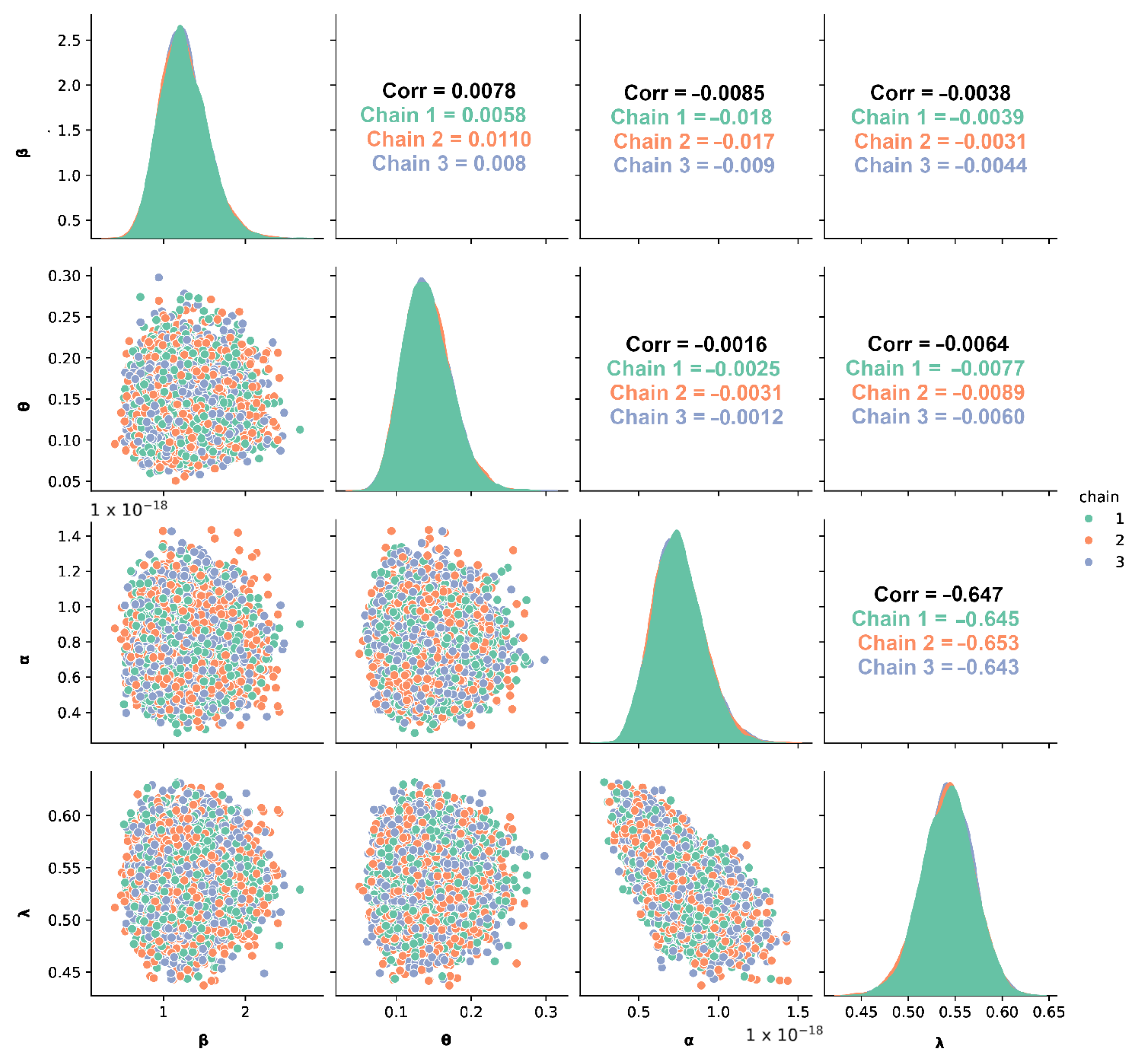
The Figure 4 shows the relationship between the parameters of the posterior sample points for the FCCR pairs and the posterior density curves of the parameters positioned along the diagonal of the scatter matrix. Regarding the form taken by the posterior densities for each HMC chain in each FCRR parameter, it is shown that they are practically symmetrical between chains, which suggests that the parameters are well-identified and that the chains have converged adequately.

In terms of the correlations between the FCCR model parameters, it is observed that most are small or negative, which favors the efficiency of BEM sampling and suggests that the different components of the model are well differentiated. This result also supports the independence assumption between the failure mechanisms considered in each electrode. From a reliability perspective, the pair $(\alpha ,\lambda )$, associated with the device wear phase (ChD), shows a high negative correlation. This indicates that, in the posterior region, an increase in $\alpha$ tends to be compensated by a decrease in $\lambda$, and vice versa. Although this suggests a close functional relationship between both parameters, their combination still adequately models the accelerated degradation phase of the electrode. On the other hand, the parameters $(\beta ,\theta )$, associated with early failures, show correlations close to zero, suggesting that failure mechanisms in the early stages of the device’s life may act independently. This reinforces the idea that different causes of failure manifest themselves with different trajectories within the system’s life cycle.

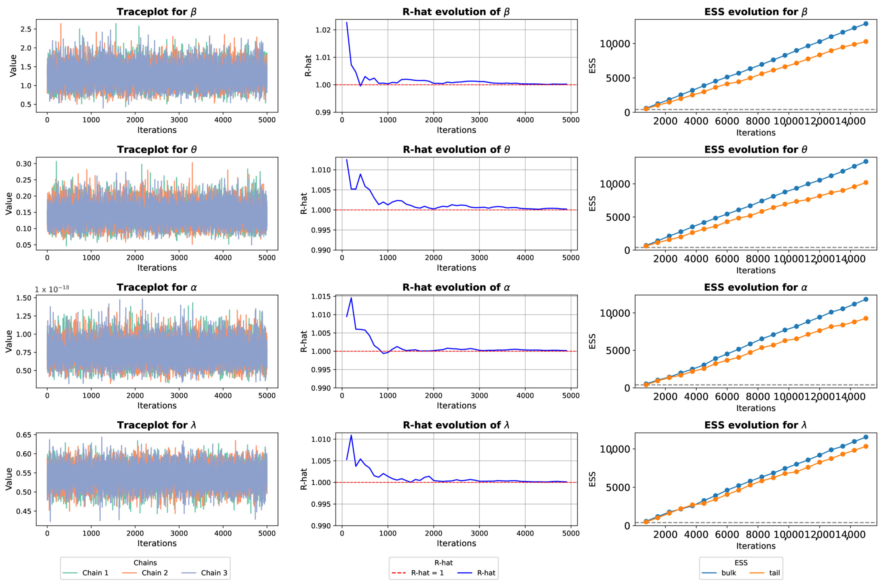
Figure 5 shows the performance of the estimates for the FCCR parameters under the BEM. The diagnosis obtained through the traceplot indicates that the patterns that seem stationary after the warm-up period, without evident trends or systematic patterns, which means that the jumps between values in the iterations show that the HMC algorithm is adequately exploring the parameter space without getting stuck in specific regions with good convergence between the parameters. This statement is supported by the graphical evolution of the $\widehat{R}\le 1.01$ and that the obtained values of the Effective Sample Size (ESS) are high, so the implementation designed in Algorithm 1 does represent the electrode data under the proposed model.

Table 3. Overview of FCCR parameter estimates from MLE and BEM in Electrode lifetime.

	Metrics	Parameters
		$\widehat{\mathit{\beta }}$	$\widehat{\mathit{\theta }}$	$\widehat{\mathit{\alpha }}$	$\widehat{\mathit{\lambda }}$
MLE	Parameter Value (StDev)	$1.715$$\left(0.125\right)$	$2.949\times {10}^{-2}(1.885\times {10}^{-3})$	$2.491\times {10}^{-7}(3.221\times {10}^{-8})$	$0.466$$\left(0.114\right)$
	$\%95CI$	$[1.470,1.960]$	$[2.579\times {10}^{-2},$$3.319\times {10}^{-2}]$	$[1.861\times {10}^{-7},$$3.122\times {10}^{-7}]$	$[0.243,0.689]$
	$KS\left(P_{K}S\right)$	$0.087$$\left(0.861\right)$	$LogLik=-263.112$	$AIC=534.224$
	$AD\left(P_{A}D\right)$	$0.275$$\left(0.877\right)$		$BIC=542.466$
	$CVM\left(P_{C}VM\right)$	$0.050$$\left(0.842\right)$		$\widehat{MTTF}=262.114$
BEM	Parameter Value (StDev)	$1.714$$\left(0.120\right)$	$2.951\times {10}^{-2}$$(1.801\times {10}^{-3})$	$2.493\times {10}^{-7}$$(3.334\times {10}^{-8})$	$0.465\left(0.113\right)$
	$\%95$HDI	$[1.479,1.949]$	$[2.599\times {10}^{-2},$$3.304\times {10}^{-2}]$	$[6.430\times {10}^{-8},$$5.155\times {10}^{-7}]$	$[0.244,0.687]$
	$\widehat{R}$	$1.0001$	$1.0000$	$1.0001$	$1.0004$
	$KS\left(P_{K}S\right)$	$0.082$$\left(0.857\right)$	$LogLik=-264.406$	$AIC=536.812$
	$AD\left(P_{A}D\right)$	$0.262$$\left(0.881\right)$		$BIC=545.054$
	$CVM\left(P_{C}VM\right)$	$0.048\left(0.853\right)$		$\widehat{MTTF}=260.847$

shows a summary of the estimates obtained for the FCCR under the MLE and BEM, as well as different evaluation metrics considered from the point of view of the reliability of the EDS. The relative difference between parameter estimates is below $2.5\%$, indicating that both methods adequately capture the performance of the electrodes under the proposed model. These slight differences do impact the information criteria: the log-likelihood and corresponding AIC and BIC values for MLE are slightly better (AIC $=534.224$, BIC $=542.466$) compared to BEM (AIC $=536.812$, BIC $=545.054$), suggesting that MLE achieves a marginally better trade-off between fit and model complexity. Nevertheless, the differences are small, and both approaches provide consistent estimates without overfitting.

These results are also reflected in the MTTF values, with MLE estimating an average electrode life of 262.114 h compared to 260.847 h under BEM. Finally, goodness-of-fit metrics presented by the KS, AD, and CVM tests show high p-values (all above $0.84$), indicating no significant evidence to reject the null hypothesis of good fit. This strongly supports the statistical validity of the FCCR model for the observed data.

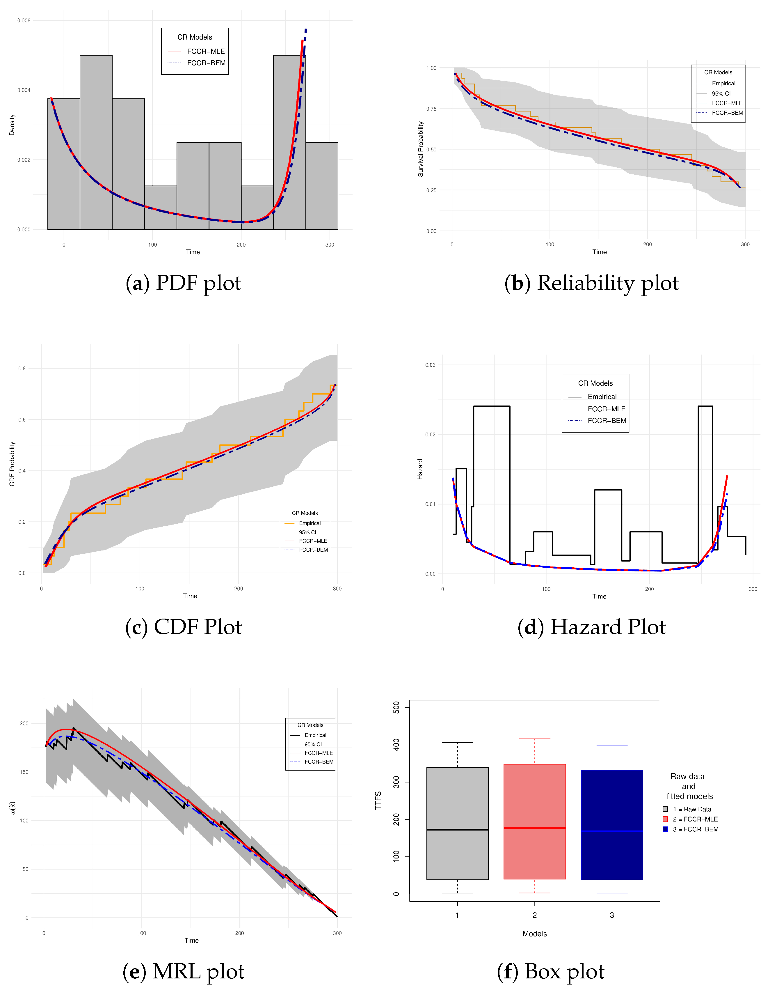
Figure 6 shows the graphic representation of the lifetimes of the electrodes, together with the securities adjusted by the FCCR model using the estimation methods by MLE and BEM. From a practical point of view, it can be seen that the shape of the PDF under the histogram follows the tendency of the data. In addition, the representations of the CDF and SF indicate that the FCCR closely follows the empirical curves generated with the Kaplan-Meier method, as for HRF, it is observed that the FCCR represents lifetimes as not monotonous, similar to the BHCR. Regarding MRL, both estimation methods offer a good adjustment, and their estimates are within the CI of $95\%$. Finally, the boxplot compares the empirical TTF with the FCCR under both estimation approaches. Significant differences between the variances of the groups (p-value = $0.6897$) suggest that both approaches properly reproduce the variability observed in the TTF.

5.1.2. Comparative Analysis of the FCCR Against Other CR Models

The evaluation of the FCCR performance is carried out through a comparative study in which other CR models were considered, which have been described in Table 2.

Table 4. Parameter estimates and summary statistics for Electrode lifetime data.

Model	P.E (SD)	Statistics
		$\mathit{L}\mathit{o}\mathit{g}\mathit{L}\mathit{i}\mathit{k}(\mathsf{\ell })$	$\mathit{A}$	$\mathit{B}$	$\mathit{K}\mathit{S}\left({\mathit{P}}_{\mathit{K}}\mathit{S}\right)$	$\mathit{A}\mathit{D}\left({\mathit{P}}_{\mathit{A}}\mathit{D}\right)$	$\mathit{C}\mathit{V}\mathit{M}\left({\mathit{P}}_{\mathit{C}}\mathit{V}\mathit{M}\right)$
FCCR	$\alpha =2.491\times {10}^{-7}$$(3.221\times {10}^{-8})$ $\lambda =0.466$$\left(0.114\right)$ $\beta =1.715$$\left(0.125\right)$ $\theta =2.949\times {10}^{-2}$$(1.885\times {10}^{-3})$	$-263.112$	$534.224$	$542.466$	$0.087$$\left(0.861\right)$	$0.275$$\left(0.877\right)$	$0.050$$\left(0.842\right)$
ACP	$\alpha =5.208\times {10}^{-5}$$(3.020\times {10}^{-3}),$ $\lambda =2.983\times {10}^{-2}$$(1.56\times {10}^{-3}),$ $\beta =1.110\times {10}^{-2}$$(3.215\times {10}^{-2}),$ $\theta =0.236$$\left(0.269\right)$	$-275.040$	$558.080$	$565.307$	$0.098$$\left(0.782\right)$	$0.498\left(0.748\right)$	$0.086$$\left(0.775\right)$
AWD	$\alpha =1.50\times {10}^{-2}$$(8.00\times {10}^{-3}),$ $\lambda =2.817$$(1.930\times {10}^{-}4)$ $\beta =8.85\times {10}^{-8}$$(1.66\times {10}^{-8})$ $\theta =0.452$$\left(0.121\right)$	$-279.517$	$567.035$	$575.276$	$0.106$$\left(0.695\right)$	$0.969$$\left(0.625\right)$	$0.114$$\left(0.652\right)$
AMW	$\alpha =1.390\times {10}^{-2}$$(1.240\times {10}^{-2}),$ $\lambda =1.591$$(1.340\times {10}^{-2}),$ $\beta =709.80$$\left(5.876\right),$ $\theta =0.377$$\left(0.183\right),$ $\gamma =7.20\times {10}^{-3}$$(1.401\times {10}^{-3})$	$-275.264$	$560.529$	$570.831$	$0.107$$\left(0.686\right)$	$0.816$$\left(0.698\right)$	$0.093$$\left(0.622\right)$
CWD	$\alpha =1.425\times {10}^{-3}$$(9.45\times {10}^{-4})$ $\lambda =4.061\times {10}^{-2}(3.086\times {10}^{-3})$ $\beta =0.328$$(1.669\times {10}^{-2})$ $\theta =0.164$$(1.112\times {10}^{-2})$	$-283.227$	$574.455$	$581.682$	$0.128$$\left(0.474\right)$	$1.569$$\left(0.510\right)$	$0.167\left(0.423\right)$
FACG	$\alpha =2.00\times {10}^{-3}(1.20\times {10}^{-3}),$ $\lambda =0.224$$(8.40\times {10}^{-2}),$ $\beta =0.323$$(1.60\times {10}^{-2}),$ $\theta =99.930$$\left(3.593\right)$	$-282.206$	$572.412$	$580.654$	$0.130$$\left(0.424\right)$	$1.703$$\left(0.477\right)$	$0.171\left(0.402\right)$
FWD	$\alpha =2.760\times {10}^{-2}$$(5.544\times {10}^{-3}),$ $\lambda =158.7$$\left(3.306\right),$ $\beta =4.266\times {10}^{-5}$$(2.358\times {10}^{-6}),$ $\theta =19.270$$\left(3.388\right)$	$-321.512$	$651.024$	$658.250$	$0.312$$\left(0.215\right)$	$2.558$$\left(0.236\right)$	$0.265\left(0.205\right)$

presents the parameter estimates for each of the models considered in Table 2, along with their respective fit statistics. Information for the FCCR model is also included, allowing a comprehensive comparison of the performance of the evaluated models. The results obtained show that the FCCR offers the highest log-likelihood value $(-263,112)$, indicating that it fits the electrode lifetimes better than the other models, where the ACP, which is its closest competitor, has a difference of more than 11 points $(-275.040)$. This difference is reflected in the fact that the AIC and BIC values are the lowest, which, from a practical point of view, shows us that the FCCR is the most parsimonious and effective model, since it achieves a good fit without resorting to an overly complex structure to describe the device’s behavior. Regarding the goodness-of-fit tests (KS, AD, and CVM), the FCCR model also stands out, presenting the lowest values for the corresponding statistics and high p-values (greater than 0.84), indicating an excellent fit of the theoretical distribution to the observed data. The second best model is the ACP, which we can also establish has a good adjustment. Still, the relative difference between the FCCR and the ACP is between 7–15%, which would prove that this degree of error comes out of the CIs that could be determined in the life of the electrode. In contrast, other models exhibit greater deviations between the fitted and empirical distributions, reflecting lower performance in this criterion.

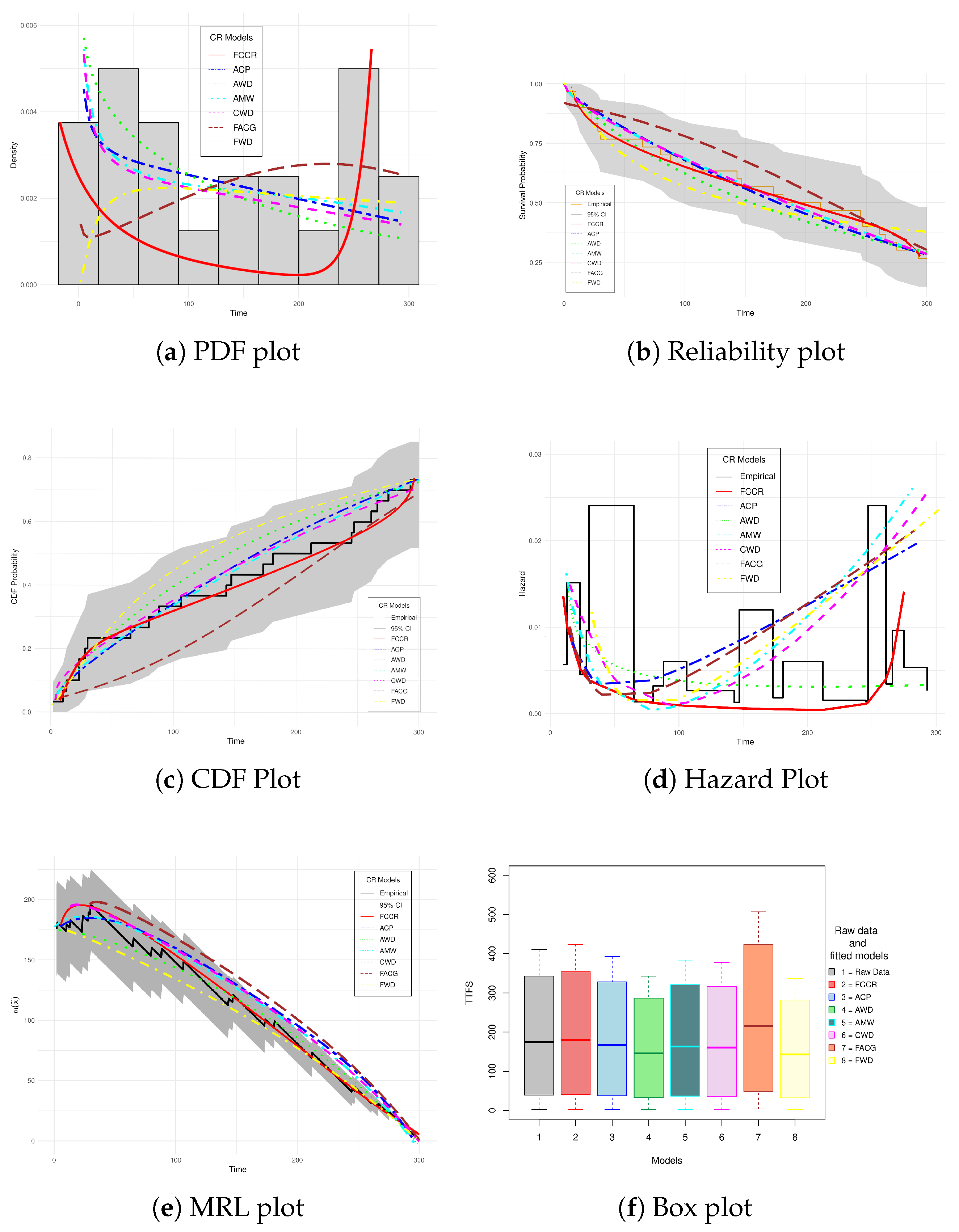
Figure 7 presents the reliability graphs of the FCCR model and the models considered in Table 2, which confirm the conclusions derived from Table 4. Furthermore, these graphs allow for a clear identification of the probability values obtained through the KS, AD, and CVM statistics, thus highlighting the practical effects of these criteria in the reliability analyses of EDs, where the impact of the shape of the reliability graphs is most evident.

Figure 7a shows the shape of the PDFs under the proposed methodology and the CR models considered for the comparative study. As can be seen, the FCCR offers a good description of the electrode behavior under real operating conditions; in turn, the ACP model provides a good fit, which indicates that the FCCR and ACP assign a higher probability to events in their optimal time range. Regarding the AWD, AMW, and CWD models, they show a greater dispersion of information, which can make them indicate failure events with a longer delay.The FACG and FWD models have noticeably lower densities than the other CR models, so that they will represent less probable events at the electrodes.

The SF shown in Figure 7b displays relevant information for practitioners to determine essential quality elements in the electrodes. As can be seen, the orange line in the graph represents the empirical reliability that the electrodes would take on under a normal usage rate; in this case, the FCCR and ACP models offer behavior close to the empirical. The AWD, AMW, and CWD models show intermediate performance, from which the practitioner can conclude whether these models would be a good option, since they have room for improvement. FWD and FACG show significant deviations, which suggests that there are failures in capturing the behavior of the electrodes.

Figure 7c shows the shape of the CDF, which allows obtaining the probability of failure of the electrodes throughout their useful life. Compared with the device’s empirical behavior, it is observed that the FCCR and ACP models fit the empirical CDF very well, offering highly competitive results. On the other hand, the AWD, AMW, ACW, and FACG models present probabilities that remain within the confidence intervals. Finally, the model with the worst performance is FWD, since it progressively moves away from both the empirical CDF and its confidence intervals.

A notable aspect of the behavior of electrode failures is demonstrated in the hazard graph shown in Figure 7d; as can be seen, the BHCR behavior is exhibited by the FCCR and the ACP; however, based on the statistics shown in Table 4, the FCCR offers a better description. Despite having BHCR properties, the other models briefly describe the normal operation stage of the electrodes, which would affect the design of the maintenance plans. Figure 7e shows the MRL of the electrodes under the different CR models. The FCCR is perceived as having a competitive performance concerning the empirical behavior, which leads to the proposed methodology more closely estimating the remaining useful life of the electrode under normal operating conditions.

Finally, the boxplot in Figure 7f shows the differences between random samples generated from the models considered in the comparative analysis and the TTFs dataset. From a practical reliability perspective, the FCCR model is similar to the original data, demonstrating the best performance among all the models considered.

Levene’s test supports this by verifying the homogeneity of variances, where the samples generally show a $p=0.0042$, indicating significant differences in the variances of all the models considered. When performing the pairwise test between the original data and each model, it was observed that the FCCR has a $p=0.746$, the ACP $p=0.737$ and the AWD $p=0.553$, which can be good candidates for the description of the electrodes throughout their useful life, since they do not present significant differences in terms of variance, which suggests a good agreement with the dispersion structure of the empirical data. The AMW models with a $p=0.116$ and the FACG $p=0.298$ are within the limits, but their performance is much lower. In contrast, the CWD $p=0.019$ and the FWD $p=0.007$ show statistically significant differences in the variance concerning the original data, which indicates a lower fit in terms of dispersion and variability of the failure times.

Taken together, these results confirm that the FCCR model fits the empirical distribution well and more faithfully reproduces the inherent variability of TTFs data compared to the other models.

Table 5. Empirical and predicted failure risks due to modes D and E for the trained models; Electrode lifetime.

Mode	Empirical Estimate	FCCR MLE	FCCR BEM	ACP	AWD	AMW	CWD	FACG	FWD
$\widehat{{\rho }_E}$	$0.40$	$0.382$	$0.385$	$0.300$	$0.254$	$0.049$	$0.179$	$0.074$	$0.157$
$\widehat{{\rho }_D}$	$0.60$	$0.618$	$0.615$	$0.700$	$0.746$	$0.951$	$0.821$	$0.928$	$0.843$

presents the probabilities of the empirical and estimated risks for each trained model for the FaMs defined for the electrode lifetimes. Empirically, it was determined that the electrodes have a probability of $60\%$ that Mode-D causes determine the FaM, and $40\%$ for the FaM defined by Mode-E. By observing the results obtained, the FCCR estimates that the FaM probabilities have $(0.618,0.382)$ for Mode-D and Mode-E, respectively, when the parameters are estimated through the MLE, and a probability of $(0.615,0.385)$ when the estimate is made using the BEM. This suggests that the FCCR model adequately captures the risk balance between the failure modes present in the part. Generally, we can establish that the ACP and AWD models correctly identify the FaM with the highest occurrence rate; however, the probabilities are higher in Mode-D, offsetting the probabilities of Mode-E.

In contrast, other models such as AMW, FACG, and CWD present significant deviations, especially in estimating Mode-E, where the predictions are significantly lower (for example, AMW predicts a risk of only 0.049 for Mode E). These deviations indicate a possible overestimation for the Mode-D and an underestimation for the Mode-E. This could have important practical implications if the model were used for maintenance decisions or failure cause prioritization. Overall, the results reflect that not all models adequately represent the empirical distribution of failure modes, with FCCR being the most robust in this specific case.

5.2. Case of Study II: Lifetimes and Downtimes of 30 Electronic Units (EUs)

This case study analyzes the behavior of 30 devices that were part of a field monitoring study as a subsystem of a larger-scale system. The experimental times were reported by Meeker et al. [50]. The methodology used to obtain the lifetimes involved subjecting the devices to real-life operating conditions with controlled stress levels. As a result of this evaluation under operating conditions, two FaMs were identified, which are described below:

• Mode S: This FaM resulted from the gradual accumulation of random damage due to voltage spikes on the power line during electrical storms, which ultimately caused a specific unprotected electronic component to fail. Such failures predominantly occurred during the early stages of the device’s operational life.
• Mode W: This FaM, resulting from typical wear and aging of the product, began to manifest after 100,000 use cycles.

Under the aforementioned FaMs, it was possible to identify that fifteen pieces experienced FaM of type S, while seven exhibited FaM characteristics of type W. The eight pieces have been censored for the analysis because they exceeded the limit of use cycles.

5.2.1. Estimation of the FCCR Model Parameters Using the MLE and BEM Approaches

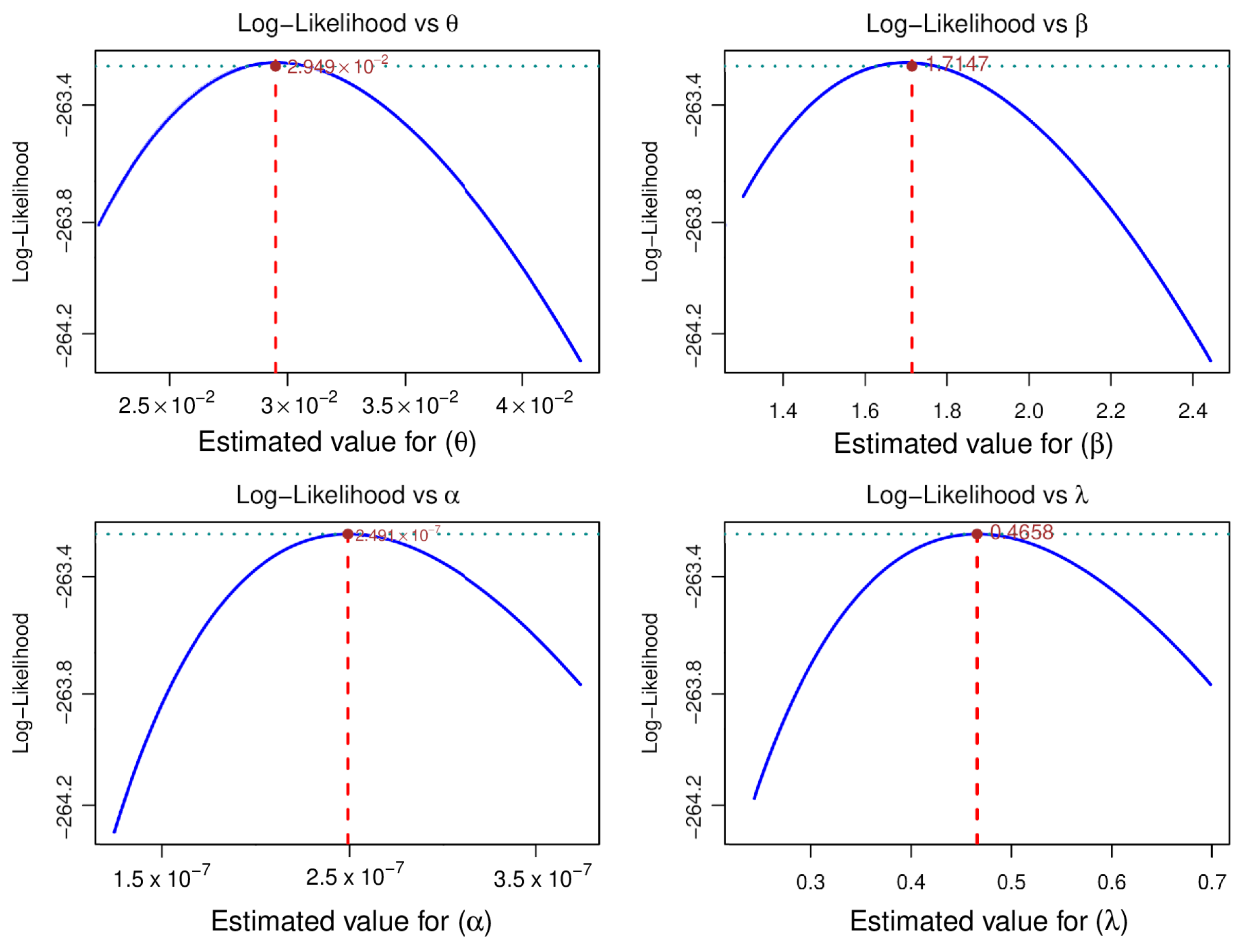
The lifetimes of these EUs were analyzed by the FCCR using two estimation approaches. First, the parameters $\beta$, $\theta$, $\alpha$, and $\lambda$ were estimated via MLE. Figure 8 displays the likelihood curves for each parameter, along with their maximizing estimates. The unimodal and concave profiles of these curves validate the robustness of the estimations.

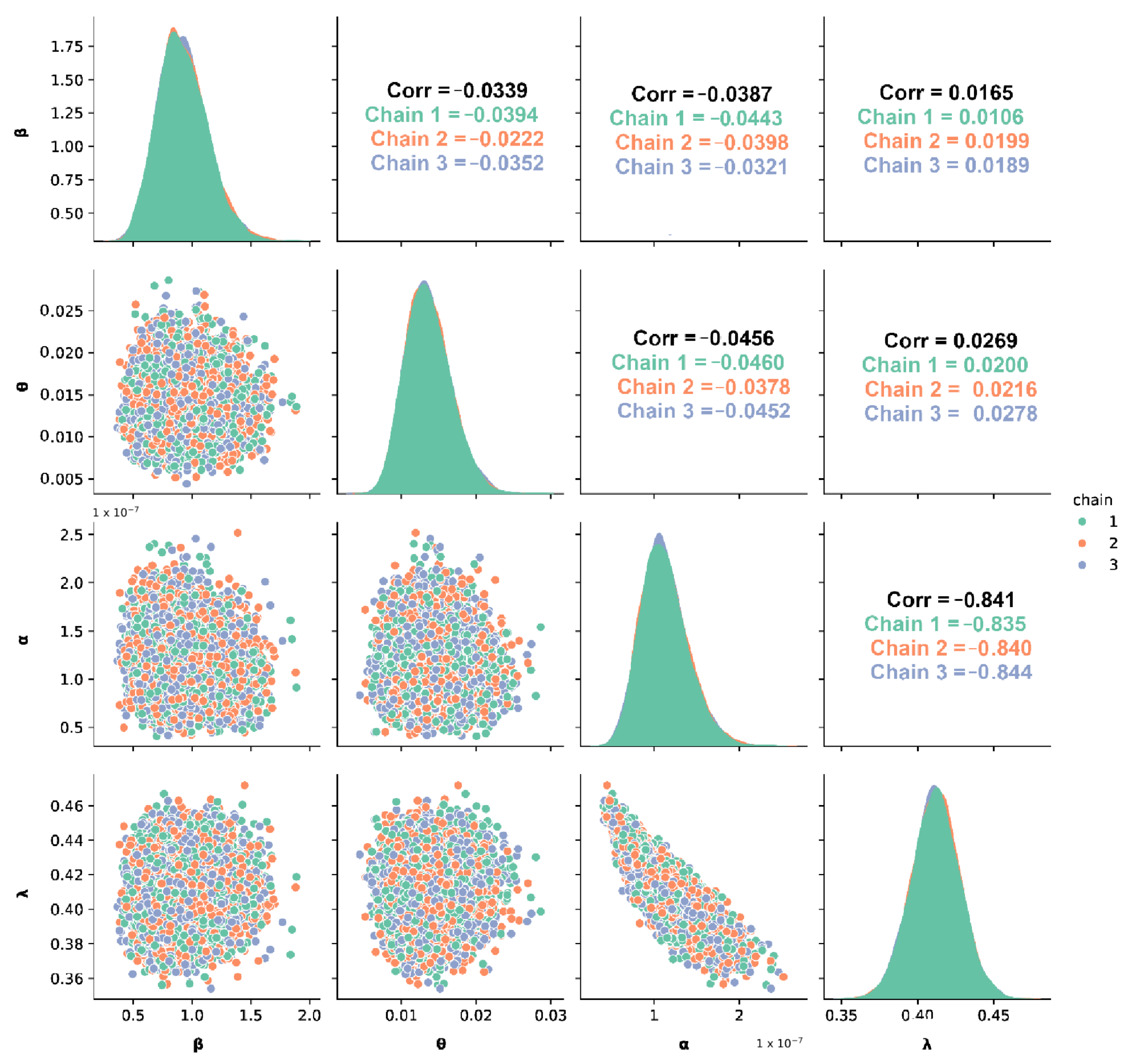
The scatterplot matrix in Figure 9 visualizes the posterior parameter dependencies for FCCR pairs, showing bivariate relationships in the off-diagonal panels and univariate kernel density estimates along the diagonal. The posterior densities for each parameter show symmetric shapes across all chains, with no evidence of observable bias; this indicates that the sampling algorithm converges adequately for the ED lifetimes analyzed in this case study. The values estimated using the BEM method are stable, ensuring robust inferences.

Regarding the correlations presented in the parameters, it can be seen that as in case study I, the pair $(\alpha ,\lambda )$ has the most negative correlation, which regulates the stage of wear in the device, so the behavior of these parameters from the practical point of view indicates how aggressive and rapid the wear is in the ED, this correlation indicates that the effects of wear are caused by causes such as the lack of preventive maintenance plans to avoid catastrophic failures in the ED, as well as external conditions that accelerate failure in the ED. The other combinations of the parameter pairs show that they are very close to zero, indicating that the FaM can remain independent under normal use conditions and with adequate maintenance plans.

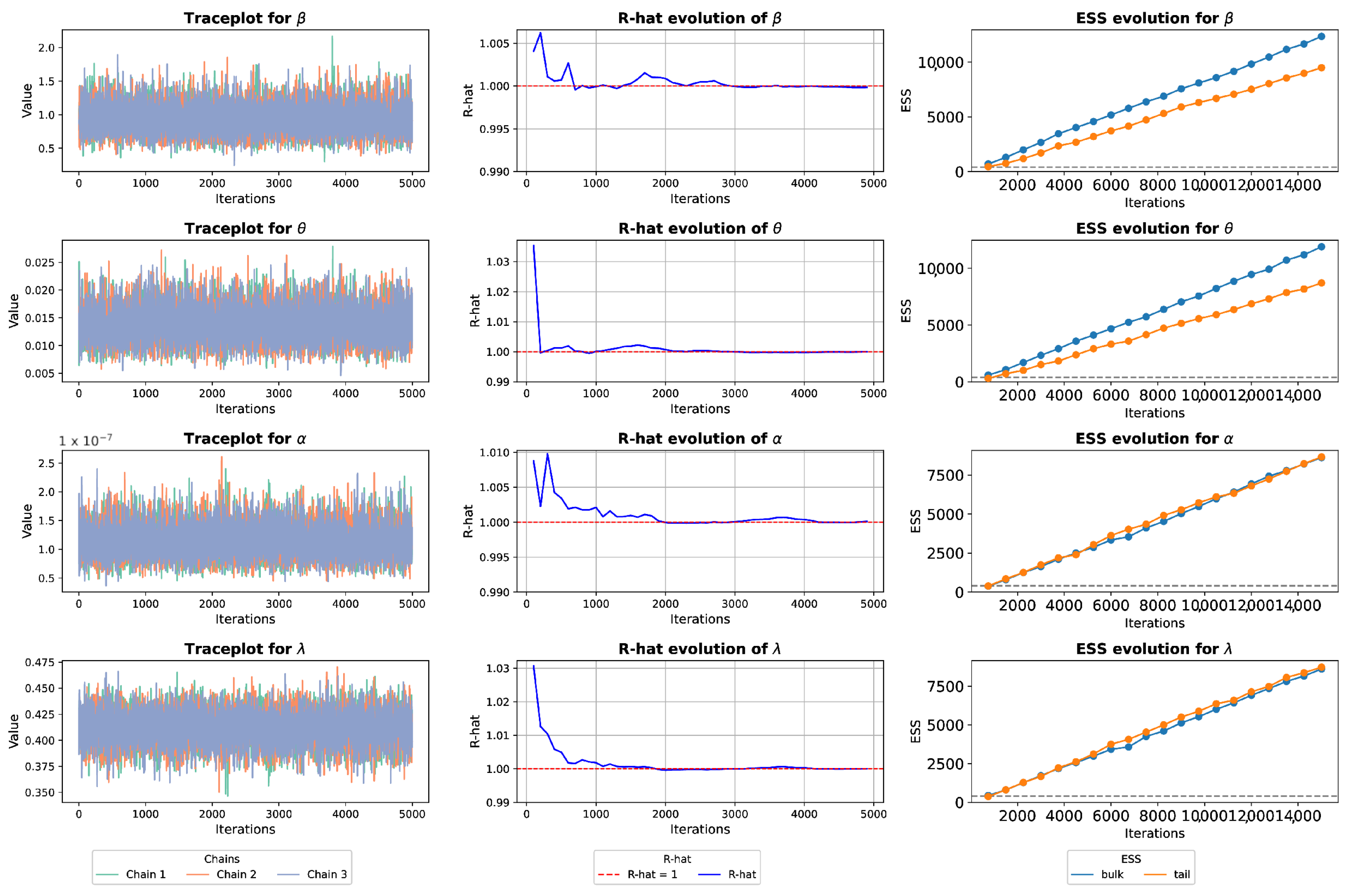
Figure 10 presents the performance graphs of the FCCR parameters estimated through the BEM. At first glance, it can be observed that the traceplot for each of the chains shows good mixing and no stationary patterns, which provides evidence that the algorithm has successfully converged. The previous statement is supported by the cumulative graph of $\widehat{R}$, where it can be seen that as the HMC chains run, the Gelman-Rubin criterion is met in all cases, that is, $\widehat{R}<1.1$. Finally, the evolution of the ESS shows high values, indicating that the chains explore the posterior space well and the parameter estimates are reliable.

Table 6. Overview of FCCR parameter estimates from MLE and BEM for EUs lifetime.

	Metrics	Parameters
		$\widehat{\mathit{\beta }}$	$\widehat{\mathit{\theta }}$	$\widehat{\mathit{\alpha }}$	$\widehat{\mathit{\lambda }}$
MLE	Parameter Value (StDev)	$1.298$$\left(0.115\right)$	$0.147$$(1.579\times {10}^{-2})$	$7.498\times {10}^{-19}$$(1.957\times {10}^{-20})$	$0.656$$\left(0.149\right)$
	$\%95CI$	$[1.0727,1.523]$	$[0.116,0.178]$	$[7.114\times {10}^{-19},$$7.882\times {10}^{-19}]$	$[0.364,0.948]$
	$KS\left(P_{K}S\right)$	$0.075$$\left(0.799\right)$	$LogLik=-132.198$	$AIC=272.396$
	$AD\left(P_{A}D\right)$	$0.249$$\left(0.815\right)$		$BIC=278.001$
	$CVM\left(P_{C}VM\right)$	$0.062$$\left(0.773\right)$	$\widehat{MTTF}=181.958$
BEM	Parameter Value (StDev)	$1.295$$\left(0.120\right)$	$0.151$$(1.329\times {10}^{-2})$	$7.495\times {10}^{-19}$$(2.798\times {10}^{-20})$	$0.655$$\left(0.158\right)$
	$\%95$HDI	$[1.060,1.530]$	$[0.125,0.177]$	$[6.946\times {10}^{-19},$$8.044\times {10}^{-19}]$	$[0.345,0.965]$
	$\widehat{R}$	$1.0002$	$1.0001$	$1.0003$	$1.0001$
	$KS\left(P_{K}S\right)$	$0.079$$\left(0.821\right)$	$LogLik=-134.356$	$AIC=276.712$
	$AD\left(P_{A}D\right)$	$0.258$$\left(0.833\right)$		$BIC=282.317$
	$CVM\left(P_{C}VM\right)$	$0.058$$\left(0.769\right)$	$\widehat{MTTF}=178.896$

summarizes the FCCR parameters for the two estimation approaches. The relative difference between the parameters is better than $3\%$. From a practical standpoint, this difference between the parameter estimates is reflected in the MTTF calculation and the fit statistics. For the MTTF, it can be seen that the FCCR-BEM is more conservative for the average life estimate, establishing that the EUs have an average life of $178.896$ h, while the FCCR-MLE establishes that the same units have $181.958$ h. These slight differences can be seen in the device reliability graphs under the two approaches.

The p-values associated with the goodness-of-fit tests (KS, AD, and CVM) for both estimation methods (MLE and BEM) are all greater than $0.77$, indicating no significant evidence to reject the hypothesis that the data originate from the fitted FCCR model. This suggests that the model adequately describes EUs’ observed lifetime behavior.

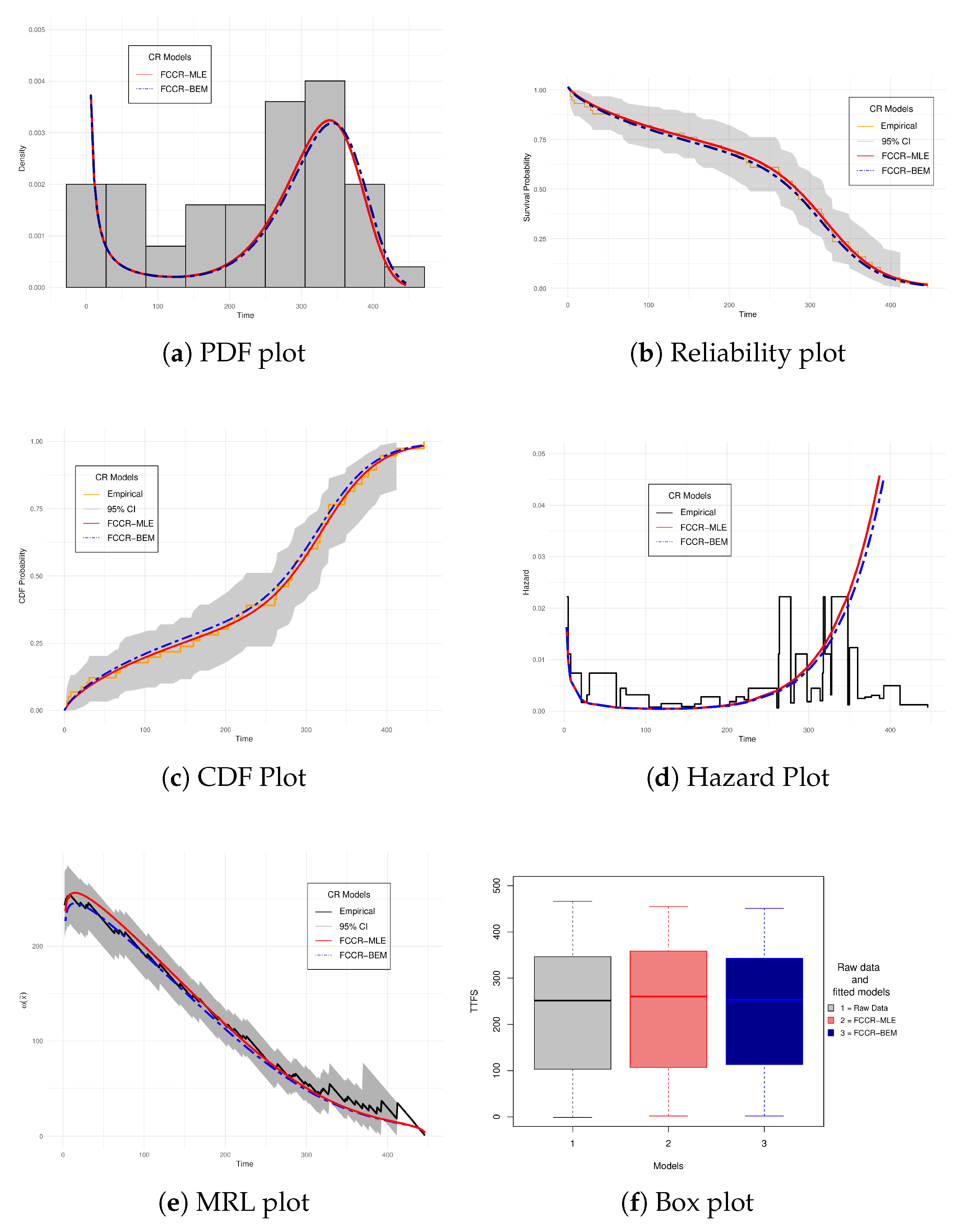
Figure 11 presents a graphical representation of the results shown in Table 6. The FCCR model, under both estimation schemes (MLE and BEM), adequately represents the lifetime behavior of the analyzed EUs. The shapes of the reliability, CDF, and MRL functions closely follow the empirical behavior estimated using the Kaplan-Meier method and remain within the confidence intervals. In the case of the HRF, it is observed that the devices exhibit a trend consistent with a BHCR.

Additionally, the boxplot comparing the empirical TTF versus those generated by both estimation methods reveals that the FCCR model, under both MLE and BEM, does not introduce significant differences in the data dispersion. This homogeneity in variability was corroborated by the Levene test, whose p-value > 0.86, supporting the hypothesis of equality of variances. This is relevant from a reliability perspective, as it suggests consistency in risk estimation without introducing additional variability through the estimation method.

5.2.2. Comparative Analysis of the FCCR Against Other CR Models

In the

Table 7. Parameter estimates and summary statistics for the EUs lifetime.

Model	P.E (SD)	Statistics
		$\mathit{L}\mathit{o}\mathit{g}\mathit{L}\mathit{i}\mathit{k}(\mathsf{\ell })$	$\mathit{A}$	$\mathit{B}$	$\mathit{K}\mathit{S}\left({\mathit{P}}_{\mathit{K}}\mathit{S}\right)$	$\mathit{A}\mathit{D}\left({\mathit{P}}_{\mathit{A}}\mathit{D}\right)$	$\mathit{C}\mathit{V}\mathit{M}\left({\mathit{P}}_{\mathit{C}}\mathit{V}\mathit{M}\right)$
FCCR	$\alpha =7.498\times {10}^{-19}$$(1.957\times {10}^{-20})$ $\lambda =0.656$$\left(0.149\right)$ $\beta =1.298$$\left(0.115\right)$ $\theta =0.147$$(1.579\times {10}^{-2})$	$-132.198$	$272.396$	$278.001$	$0.075$$\left(0.799\right)$	$0.249$$\left(0.815\right)$	$0.062$$\left(0.773\right)$
ACP	$\alpha =1.314$$\left(0.119\right),$ $\lambda =1.563\times {10}^{-3}$$(8.667\times {10}^{-4}),$ $\beta =9.957\times {10}^{-3}$$(1.690\times {10}^{-4}),$ $\theta =0.267$$(3.350\times {10}^{-3})$	$-142.506$	$293.013$	$297.3777$	$0.026$$\left(0.375\right)$	$0.032$$\left(0.393\right)$	$0.039$$\left(0.366\right)$
AWD	$\alpha =8.150\times {10}^{-3}$$(9.275\times {10}^{-4}),$ $\lambda =0.878$$\left(0.204\right)$ $\beta =7.323\times {10}^{-3}$$(9.610\times {10}^{-4})$ $\theta =3.048\times {10}^{-2}$$(4.024\times {10}^{-3})$	$-142.878$	$293.756$	$298.120$	$0.0178$$\left(0.280\right)$	$0.006$$\left(0.299\right)$	$0.0013$$\left(0.245\right)$
AMW	$\alpha =1.471\times {10}^{-2}$$(9.422\times {10}^{-3}),$ $\lambda =0.342$$(2.951\times {10}^{-3}),$ $\beta =116.971$$\left(0.857\right),$ $\theta =0.654$$\left(0.197\right),$ $\gamma =2.411\times {10}^{-3}$$(1.415\times {10}^{-3})$	$-141.869$	$293.738$	$300.744$	$0.019$$\left(0.278\right)$	$0.016$$\left(0.299\right)$	$0.014$$\left(0.257\right)$
CWD	$\alpha =1.391\times {10}^{-2}$$(5.831\times {10}^{-3})$ $\lambda =1.732\times {10}^{-2}$$(3.296\times {10}^{-3})$ $\beta =0.260$$(2.056\times {10}^{-2})$ $\theta =0.150$$(1.874\times {10}^{-2})$	$-143.037$	$294.074$	$298.438$	$0.132$$\left(0.521\right)$	$2.676$$\left(0.545\right)$	$0.138$$\left(0.501\right)$
FACG	$\alpha =1.302\times {10}^{-2}$$(1.447\times {10}^{-3}),$ $\lambda =0.722$$(4.558\times {10}^{-2}),$ $\beta =0.267$$(2.558\times {10}^{-2}),$ $\theta =289.99$$\left(7.114\right)$	$-142.119$	$292.236$	$297.843$	$0.025$$\left(0.347\right)$	$0.020$$\left(0.377\right)$	$0.037$$\left(0.297\right)$
FWD	$\alpha =2.760\times {10}^{-2}$$(5.544\times {10}^{-3}),$ $\lambda =158.7$$\left(3.306\right),$ $\beta =4.266\times {10}^{-5}$$(2.358\times {10}^{-6}),$ $\theta =19.270$$\left(3.388\right)$	$-151.512$	$311.024$	$316.629$	$0.312$$\left(0.215\right)$	$2.558$$\left(0.236\right)$	$0.265$$\left(0.205\right)$

, the results of the parameters for CR models are presented when performing the lifetimes of the EUs. From the statistical point of view, the FCCR model stands out for achieving the highest value of log-likelihood $(-132.198)$, which correlates with the lower AIC values $\left(272.396\right)$ and BIC $\left(278.001\right)$. This indicates that the FCCR not only has greater explanatory capacity, but also efficiently penalizes the complexity in the behavior of the units compared to the other competitive models. The closest models in log-likelihood are the FACG $\left(292.236\right)$ and the AMW $\left(293.738\right)$, although with significant differences.

Regarding adjustment goodness tests, the FCCR shows the best performance, with the highest values in all metrics: KS (p-value = 0.799), AD (p-value = 0.815), and CVM (p-value = 0.773), which suggests an optimal adjustment without significant discrepancies. In contrast, although the AWD has lower statistics (KS = 0.0178) and lower p-values (Ks = 0.280, Ad = 0.299, CVM = 0.245), it is less viable for practical applications in this context. Among the alternative models, the CWD presents the best performance after the FCCR, according to the criteria evaluated. Figure 12 shows the shapes taken by the reliability graphs with the estimated values in Table 7 and the lifetimes of the EUs.

Figure 12a presents the PDF shapes for each model studied. From a practical perspective, it can be observed that the FCCR offers a good representation concerning the histogram of the analyzed data, which confirms the statistics obtained in Table 7.

The SF graph in Figure 12b shows that the FCCR more closely follows the empirical behavior expressed by the EUs’ lifetimes. It is also possible to observe that the ACP, AMW, and CWD models are very close competitors and can offer important information for improving the ED or for establishing maintenance plans or guarantees for the ED under the operating conditions for which it was designed. It is also observed that, although other models considered, such as the FACG and the FWD, are within the limits of the Kaplan-Meier CI, their fit is poor, since they fail to adequately capture the general trend of the empirical curve.

A similar behavior can be seen in the CDF representation shown in Figure 12c, where the FCCR model shows a competitive advantage over the rest of the CR models. Models such as ACP, AWD, and CWD achieve a reasonable fit in the initial part of the empirical curve; however, they fail to capture the inflection points of the observed distribution adequately. The remaining models tend to fit in the extreme regions, but their overall performance is unsatisfactory despite being within the confidence interval.

Figure 12d shows the shape of the failure times of the EUs, clearly highlighting the capacity of the FCCR model compared to the other CR models. In particular, the FCCR allows for the representation of a failure rate behavior in the form of a BHCR, in which the three classic stages are distinguished: infant mortality, operational useful life, and final wear. This characteristic is especially useful from a practical point of view, since it facilitates the identification of the point of onset of early mortality, the period of stable operation, and the beginning of the aging phase, which allows specialists to define optimal maintenance plans to extend the useful life of the equipment. In contrast, the other CR models present an irregular representation of the BHCR or cannot model non-monotonic behaviors, demonstrating their lower flexibility in describing failure processes with a bathtub structure.

Figure 12e compares the MRL function estimated by each model and the empirical behavior. Once again, it is seen that the FCCR model presents the greatest agreement with the observed trend, which suggests that the estimate of the replacement rate of the EUs under this model is the most representative of the real operating conditions for which they were designed. In this sense, the AMW model constitutes the second-best alternative in terms of proximity to the empirical behavior. On the other hand, models such as FACG, FWD, and AWD, although they coincide with the empirical curve in certain sections, show significant deviations in others, as they are outside the CI range. This indicates that, from a practical perspective, their estimates may be biased and, therefore, less reliable for decision-making.

Finally, Figure 12f presents the boxplots for each CR model evaluated in this case study, comparing them regarding device lifetimes. The objective is to illustrate the variability of the random samples generated by the models and assess their similarity to the ED dataset. The results indicate that the sample distribution produced by the FCCR model closely aligns with the raw data. Levene’s test was applied to assess the homogeneity of variances among the TTFs estimated by the different models, yielding an overall p-value of 0.0354. This provides statistically significant evidence to reject the null hypothesis of equal variances, indicating that the variability in TTFs across the models is not homogeneous.

In the individual analysis, the FCCR model exhibits a p-value of 0.845, the highest among all CR models evaluated, suggesting greater consistency in the dispersion of its estimates concerning the empirical data. Other models with relatively high p-values include ACP (0.773), AMW (0.662), and CWD (0.591). However, a high p-value in this test does not necessarily imply a good overall fit. Therefore, practitioners should consider the overall performance of each model by examining the various graphical representations shown in Figure 12, to comprehensively evaluate their ability to describe the behavior of the device under study.

The risk associated with the two FaMs for the EDs in this case study is presented in

Table 8. Empirical and predicted failure risks due to modes S and W for the trained models; EUs lifetime.

Mode	Empirical Estimate	FCCR MLE	FCCR BEM	ACP	AWD	AMW	CWD	FACG	FWD
$\widehat{{\rho }_S}$	$0.682$	$0.680$	$0.675$	$0.602$	$0.518$	$0.785$	$0.558$	$0.998$	$0.595$
$\widehat{{\rho }_W}$	$0.318$	$0.320$	$0.325$	$0.398$	$0.518$	$0.215$	$0.442$	$0.002$	$0.405$

. Empirically, it was estimated that for Mode-S the probability is $0.682$ and for Mode-W it is $0.318$. It is seen that the FCCR under the MLE offers a probability of $0.680$ and $0.320$ for Modes S and W, respectively. Likewise, the FCCR under BEI offers results that are very close to the empirical estimates, so the FCCR represents the probability of the risk for the ED under analysis well.

The ACP model also correctly identifies FaMs with some degree of equilibrium, but underestimates the Mode-S FaM, which leads to bias. The AMW model is reasonably fit but tends to overestimate the Mode-S FaM. The AWD model considered that the FaMs have the same probability of failure, which is reasonable since the AWD model considers that a WD represents both FaMs. The CWD and FWD models underestimate the Mode-S FaM and inflate the Mode-W FaM compared to the real data, indicating that these models have high deviation. Finally, FACG assigns almost all FaMs to Mode-S, severely underestimating the wear mode.

Therefore, from a practical perspective, the FCCR model shows excellent performance concerning the statistical fit values, a good graphical representation of the EUs, and an adequate calculation of the FaM risk probability within the analyzed device.

6. Physical Interpretation of FCCR Model Parameters in Reliability Analysis

An essential element when proposing methodologies to describe EDs lifetimes within the scope of reliability is the interpretation of how parameters affect the performance and FaM of the device under analysis.

A literature review on predictive reliability models shows that many authors overlook this practical aspect. As a result, the proposed models frequently lack generalization capabilities and are valid only for the specific case studies in which they are implemented. This limitation represents an area of opportunity that the FCCR model systematically explores to provide practitioners with key data for decision-making. These decisions can range from design improvements to implementing preventive maintenance plans and predicting optimal operating conditions, thus ensuring the proper functioning of EDs.

Based on the results obtained from the analyzed case studies, a practical interpretation of the FCCR model parameters can be provided as follows:

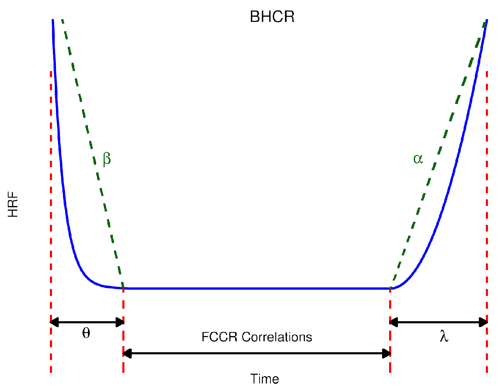
• $\beta$ (burn-in shape): represents the infant mortality stage, which will be found on the left side of the BHCR. Its estimated value will indicate how pronounced the exponential drop in this stage of the ED will be. $\beta$ in design environments, regulates the ED warranty times.
• $\theta$ (burn-in scale): gives practitioners the rate at which the device reaches normal use life, i.e., how quickly the ED matures and survives the effects of manufacturing and/or design processes.
• $\alpha$ (fatigue shape): controls the wear stage in the ED. This means it establishes the probability that the device’s internal components will fail to maintain optimal functioning before a catastrophic failure occurs. In the case of the BCHR representation, $\alpha$ is in the exponentially growing stage of said representation.
• $\lambda$ (fatigue scale): within the FCCR modulates how internal components lose physical and design properties to maintain full ED operation. This parameter is located in the exponentially increasing part of the BHCR.
• The correlations, except $(\alpha ,\lambda )$ and $(\beta ,\theta )$, are represented in the flat part of the graph (BHCR), which indicates the possible failures that may occur in the device as a consequence of the interactions that the internal components of the ED have.

Figure 13 shows the location and effect of the FCCR parameters on the HRF and BHCR for the EDs in reliability analysis cases. These elements allow reliability specialists to understand better how estimates influence the useful life of EDs, thus facilitating the optimization of warranty and maintenance plans.

7. Conclusions and Future Work

This paper presents a reliability model called FCCR to analyze EDs lifetimes. Among the characteristics of the proposed model is the representation of ED failures when these follow a monotonic, nonmonotonic, or both behaviors simultaneously. The model was built using the CR methodology, integrating the minimum variables of the FrD and ChD distributions. Using the methodological framework allows for a more flexible representation in datasets where two FaMs coexist, a context in which traditional reliability models have limitations. The assumptions on which the FCCR has been developed are that the two FaMs are considered independent in the ED, that is, the failure does not depend on another failure, and the events are mutually exclusive, which means that when a failure occurs, the others are discarded when recording the time of the event in the device. As limitations of the model are that in case of a high positive correlation, these affect the full identification of the cause of the FaM, the data are censored because they exceed the test time, and not because of a failure related to the device, and only the two most frequent FaMs in the ED are considered. All assumptions and limitations are specific to the CR methodology.

From a practical perspective in reliability analysis, essential mathematical properties have been presented and discussed to describe the behavior of EDs under design environments. These properties include moments, MTTF, and risk analysis to calculate the probability of FaM occurring during ED operation. Two approaches have been proposed for estimating FCCR parameters: the classical MLE approach and the use of BEM, which, through the HMC algorithm, made it possible to generate posterior samples to handle complex distributions and offer greater efficiency in parameter inference.

Two case studies were presented to verify the proposed model. The FCCR was compared statistically and from a reliability perspective with six other state-of-the-art models that share similar conditions and properties. The EDs considered in both cases exhibit dual FaM in their respective datasets and monotonic and nonmonotonic behaviors similar to those represented by the BHCR.

The results obtained from the case studies provide strong evidence for reliability practitioners regarding the applicability of the FCCR model in the analysis of EDs’ lifetimes. The summaries presented in Table 4 and Table 7 demonstrate that the proposed model exhibits competitive and in many cases superior performance compared to other models reported in the current literature, as supported by the corresponding statistical indicators. Moreover, the reliability curves shown in Figure 7 and Figure 12 reveal that the FCCR closely aligns with the empirical curves of the PDF, SF, CDF, and MRL, reinforcing the consistency of the statistical outcomes. Finally, the risk probabilities reported in Table 5 and Table 8 indicate that the FCCR accurately captures the failure associated with each FaM observed in the EDs. From a practical standpoint, these results highlight the FCCR’s ability to provide a robust balance between statistical estimation, graphical fit, and the computation of failure risk probabilities.

A fundamental contribution of this paper is the interpretation of the effects of the FCCR parameters on the reliability analysis of EDs. This interpretation concludes that $\beta ,\theta$ control the manner and speed at which the ED acts during its initial life stage. $\alpha ,\lambda$ modulate the shape and speed at which the ED suffers wear.

As a possible line of future work, extending the FCCR model to incorporate the modeling of a third FaM is proposed. To do this, the fault events in the piece can be represented by a vector and integrated through a location-scaling parameter into a regression scheme. This extension would allow greater flexibility in representing more complex fault patterns, in which more than two FaMs coexist. Another possible extension of the FCCR model is its incorporation into the Accelerated Life Testing framework, which is widely used in reliability studies to obtain data over short periods. For this purpose, classic models such as the Inverse Power Law or the Arrhenius model can be considered; these are the most common models used in ED life analysis due to the influence of acceleration variables such as voltage and temperature, respectively. These models can be implemented through functional substitution of the parameters $\lambda$ and $\theta$, thus allowing.

References

1. Jones, H.W. Reliability Growth Modeling and Testing. In Proceedings of the 2025 Annual Reliability and Maintainability Symposium (RAMS), Miramar Beach, FL, USA, 27–30 January 2025; pp. 1–5. [Google Scholar]
2. Al Mutairi, A.; Iqbal, M.Z.; Arshad, M.Z.; Alnssyan, B.; Al-Mofleh, H.; Afify, A.Z. A new extended model with bathtub-shaped failure rate: Properties, inference, simulation, and applications. Mathematics 2021, 9, 2024. [Google Scholar] [CrossRef]
3. Sindhu, T.N.; Anwar, S.; Hassan, M.K.; Lone, S.A.; Abushal, T.A.; Shafiq, A. An analysis of the new reliability model based on bathtub-shaped failure rate distribution with application to failure data. Mathematics 2023, 11, 842. [Google Scholar] [CrossRef]
4. Wang, K.; Hsu, F.; Liu, P. Modeling the bathtub shape hazard rate function in terms of reliability. Reliab. Eng. Syst. Saf. 2002, 75, 397–406. [Google Scholar] [CrossRef]
5. Ikonen, T.J.; Mostafaei, H.; Ye, Y.; Bernal, D.E.; Grossmann, I.E.; Harjunkoski, I. Large-scale selective maintenance optimization using bathtub-shaped failure rates. Comput. Chem. Eng. 2020, 139, 106876. [Google Scholar] [CrossRef]
6. Jiang, R. A new bathtub curve model with a finite support. Reliab. Eng. Syst. Saf. 2013, 119, 44–51. [Google Scholar] [CrossRef]
7. Li, C.; Cheng, J.; Zhu, H.; Wen, B.; Zhao, X.; Kang, W. Degradation modeling and remaining useful life prediction for electronic device under multiple stress influences. Sci. Rep. 2025, 15, 19117. [Google Scholar] [CrossRef]
8. Friederich, J.; Lazarova-Molnar, S. Reliability assessment of manufacturing systems: A comprehensive overview, challenges and opportunities. J. Manuf. Syst. 2024, 72, 38–58. [Google Scholar] [CrossRef]
9. Lai, C.; Xie, M.; Murthy, D. A modified Weibull distribution. IEEE Trans. Reliab. 2003, 52, 33–37. [Google Scholar] [CrossRef]
10. El-Morshedy, M.; El-Dawoody, M.; El-Faheem, A.A. Symmetric and Asymmetric Expansion of the Weibull Distribution: Features and Applications to Complete, Upper Record, and Type-II Right-Censored Data. Symmetry 2025, 17, 131. [Google Scholar] [CrossRef]
11. Reddy, G.H.; Koundinya, A.N.; Gope, S.; Behera, C. Lifetime estimation of electrical equipment in distribution system using modified 3-parameter Weibull distribution. In Proceedings of the 2021 International Conference on Design Innovations for 3Cs Compute Communicate Control (ICDI3C), Bangalore, India, 10–11 June 2021; pp. 21–26. [Google Scholar]
12. Shama, M.S.; Alharthi, A.S.; Almulhim, F.A.; Gemeay, A.M.; Meraou, M.A.; Mustafa, M.S.; Hussam, E.; Aljohani, H.M. Modified generalized Weibull distribution: Theory and applications. Sci. Rep. 2023, 13, 12828. [Google Scholar] [CrossRef]
13. Lemonte, A.J. A new exponential-type distribution with constant, decreasing, increasing, upside-down bathtub and bathtub-shaped failure rate function. Comput. Stat. Data Anal. 2013, 62, 149–170. [Google Scholar] [CrossRef]
14. Arshad, M.; Khetan, M.; Kumar, V.; Pathak, A.K. Record-based transmuted generalized linear exponential distribution with increasing, decreasing and bathtub shaped failure rates. Commun. Stat.-Simul. Comput. 2024, 53, 3489–3513. [Google Scholar] [CrossRef]
15. Sarhan, A.M.; Zaindin, M. Modified Weibull distribution. APPS. Appl. Sci. 2009, 11, 123–136. [Google Scholar]
16. Khalil, A.; Ijaz, M.; Ali, K.; Mashwani, W.K.; Shafiq, M.; Kumam, P.; Kumam, W. A novel flexible additive Weibull distribution with real-life applications. Commun. Stat.-Theory Methods 2021, 50, 1557–1572. [Google Scholar] [CrossRef]
17. Wang, L.; Wu, K.; Tripathi, Y.M.; Lodhi, C. Reliability analysis of multicomponent stress–strength reliability from a bathtub-shaped distribution. J. Appl. Stat. 2022, 49, 122–142. [Google Scholar] [CrossRef]
18. Ghazal, M. A new extension of the modified Weibull distribution with applications for engineering data. Probabilistic Eng. Mech. 2023, 74, 103523. [Google Scholar] [CrossRef]
19. Xie, M.; Tang, Y.; Goh, T.N. A modified Weibull extension with bathtub-shaped failure rate function. Reliab. Eng. Syst. Saf. 2002, 76, 279–285. [Google Scholar] [CrossRef]
20. Mohammad, H.H.; Alamri, F.S.; Salem, H.N.; EL-Helbawy, A.A. The Additive Xgamma-Burr XII Distribution: Properties, Estimation and Applications. Symmetry 2024, 16, 659. [Google Scholar] [CrossRef]
21. Thach, T.T. A three-component additive weibull distribution and its reliability implications. Symmetry 2022, 14, 1455. [Google Scholar] [CrossRef]
22. He, B.; Cui, W.; Du, X. An additive modified Weibull distribution. Reliab. Eng. Syst. Saf. 2016, 145, 28–37. [Google Scholar] [CrossRef]
23. Liao, Q.; Ahmad, Z.; Mahmoudi, E.; Hamedani, G. A New Flexible Bathtub-Shaped Modification of the Weibull Model: Properties and Applications. Math. Probl. Eng. 2020, 2020, 3206257. [Google Scholar] [CrossRef]
24. Sarhan, A.M.; Hamilton, D.C.; Smith, B. Statistical analysis of competing risks models. Reliab. Eng. Syst. Saf. 2010, 95, 953–962. [Google Scholar] [CrossRef]
25. Singh, B. An additive Perks–Weibull model with Bathtub-shaped hazard rate function. Commun. Math. Stat. 2016, 4, 473–493. [Google Scholar] [CrossRef]
26. Dutta, S.; Ng, H.K.T.; Kayal, S. Inference for a general family of inverted exponentiated distributions under unified hybrid censoring with partially observed competing risks data. J. Comput. Appl. Math. 2023, 422, 114934. [Google Scholar] [CrossRef]
27. Shi, H.; Wei, C.; Zhang, Z.; Liu, B.; Wen, Y. Belief reliability analysis of competing for failure systems with bi-uncertain variables. J. Ambient. Intell. Humaniz. Comput. 2021, 12, 10651–10665. [Google Scholar] [CrossRef]
28. Shi, H.; Wei, C.; Zhang, Z.; Liu, B.; Wen, Y. Reliability analysis of dependent competitive failure model with uncertain parameters. Soft Comput. 2022, 26, 33–43. [Google Scholar] [CrossRef]
29. Yang, Z.; Li, X.; Chen, C.; Zhao, H.; Yang, D.; Guo, J.; Luo, W. Reliability assessment of the spindle systems with a competing risk model. Proc. Inst. Mech. Eng. Part O J. Risk Reliab. 2019, 233, 226–234. [Google Scholar] [CrossRef]
30. Muhammad, M.; Abba, B.; Xiao, J. Approximate Bayesian computation for a dual-failure-modes models and its application to failure times data. IEEE Access 2025, 13, 50635–50651. [Google Scholar] [CrossRef]
31. Abba, B.; Wang, H.; Bakouch, H.S. A reliability and survival model for one and two failure modes system with applications to complete and censored datasets. Reliab. Eng. Syst. Saf. 2022, 223, 108460. [Google Scholar] [CrossRef]
32. Fréchet, M. Sur la loi de probabilité de l’écart maximum. Ann. Soc. Polonaise Math. 1927. Available online: https://cir.nii.ac.jp/crid/1572261550191409280 (accessed on 14 August 2025).
33. Alzawq, F.S.A.; ElKholy, A.K. The generalized feéchet distribution with variable hazard rate shapes: Properties and applications. Pak. J. Stat. 2023, 39, 387–414. [Google Scholar]
34. Baharith, L.A. A new generalization of the exponentiated Frechet distribution with applications. J. Reliab. Stat. Stud. 2022, 15, 129–152. [Google Scholar] [CrossRef]
35. Deka, D.; Das, B.; Baruah, B.K.; Baruah, B. Some properties on Fréchet-Weibull distribution with application to real life data. Math Stat 2021, 9, 8–15. [Google Scholar] [CrossRef]
36. Chen, Z. A new two-parameter lifetime distribution with bathtub shape or increasing failure rate function. Stat. Probab. Lett. 2000, 49, 155–161. [Google Scholar] [CrossRef]
37. Méndez-González, L.C.; Rodríguez-Picón, L.A.; Rodríguez Borbón, M.I.; Sohn, H. The Chen–Perks Distribution: Properties and Reliability Applications. Mathematics 2023, 11, 3001. [Google Scholar] [CrossRef]
38. Méndez-González, L.C.; Rodríguez-Picón, L.A.; Pérez-Olguín, I.J.C.; Vidal Portilla, L.R. An additive chen distribution with applications to lifetime data. Axioms 2023, 12, 118. [Google Scholar] [CrossRef]
39. Thanh Thach, T.; Briš, R. An additive Chen-Weibull distribution and its applications in reliability modeling. Qual. Reliab. Eng. Int. 2021, 37, 352–373. [Google Scholar] [CrossRef]
40. Viswakala, K.; Abdul Sathar, E. Classical estimation of hazard rate and mean residual life functions of Pareto distribution. Commun. Stat.-Theory Methods 2019, 48, 4367–4379. [Google Scholar] [CrossRef]
41. Škanata, D. Asymptotic properties of the hazard function and the mean residual life function. WSEAS Trans. Math. 2020, 19, 275–279. [Google Scholar] [CrossRef]
42. Iscioglu, F. A new approach in the mean residual lifetime evaluation of a multi-state system. Proc. Inst. Mech. Eng. Part O J. Risk Reliab. 2021, 235, 700–710. [Google Scholar] [CrossRef]
43. Volf, P. A Statistical Model of Hazard Rate Change Caused by a Random Shock. Int. J. Reliab. Qual. Saf. Eng. 2024, 31, 2450021. [Google Scholar] [CrossRef]
44. Kharazmi, O.; Balakrishnan, N. Cumulative residual and relative cumulative residual Fisher information and their properties. IEEE Trans. Inf. Theory 2021, 67, 6306–6312. [Google Scholar] [CrossRef]
45. H. Olcay, A. Mean residual life function for certain types of non-monotonic ageing. Commun. Statistics. Stoch. Model. 1995, 11, 219–225. [Google Scholar] [CrossRef]
46. Gelman, A.; Lee, D.; Guo, J. Stan: A probabilistic programming language for Bayesian inference and optimization. J. Educ. Behav. Stat. 2015, 40, 530–543. [Google Scholar] [CrossRef]
47. Henningsen, A.; Toomet, O. maxLik: A package for maximum likelihood estimation in R. Comput. Stat. 2011, 26, 443–458. [Google Scholar] [CrossRef]
48. Stan Development Team. RStan: The R Interface to Stan, 2025. R Package Version 2.32.7. 2025. Available online: https://cran.r-project.org/web/packages/rstan/index.html (accessed on 14 August 2025).
49. Deganaksoy, N.; Hahn, G.; Meeker, W. Reliability analysis by failure mode—A useful tool for product reliability evaluation and improvement. Qual. Prog. 2002, 35, 47–52. [Google Scholar]
50. Meeker, W.Q.; Escobar, L.A.; Pascual, F.G. Statistical Methods for Reliability Data; John Wiley & Sons: Hoboken, NJ, USA, 2021. [Google Scholar]
Figure 1. HRF shapes derived from the FCCR model for various parameter configurations.
Electronics 14 03276 g001
Figure 2. Different patterns of the MRL associated with specific HRF behaviors are depicted in Figure 1.
Electronics 14 03276 g002
Figure 3. Profile log-likelihood functions of the FCCR parameters for electrode lifetime.
Electronics 14 03276 g003
Figure 4. Scatter plot matrix of FCCR parameter pairs derived from HMC posterior samples for Electrode lifetime.
Electronics 14 03276 g004
Figure 5. Trace plot, R-hat evoultion and ESS Evolution for FCCR under HMC posterior samples for Electrode lifetime.
Electronics 14 03276 g005
Figure 6. Reliability Plots for FCCR under MLE and BEM for Electrode lifetime.
Electronics 14 03276 g006
Figure 7. Reliability Plots for Each Estimation Approach of the CR Models on Electrode lifetime.
Electronics 14 03276 g007
Figure 8. Profile log-likelihood functions for the FCCR parameters for EUs lifetime.
Electronics 14 03276 g008
Figure 9. Scatter plot matrix of FCCR parameter pairs derived from HMC posterior samples for EUs lifetime.
Electronics 14 03276 g009
Figure 10. Trace plot, R-hat evoultion and ESS Evolution for FCCR under HMC posterior samples for EUs lifetime.
Electronics 14 03276 g010
Figure 11. Reliability Plots for FCCR under MLE and BEM for EUs lifetime.
Electronics 14 03276 g011
Figure 12. Reliability Plots for Each Estimation Approach of the CR Models on EUs lifetime.
Electronics 14 03276 g012
Figure 13. Identification of FCC parameters in the BHCR.
Electronics 14 03276 g013