Accelerating High-Frequency Circuit Optimization Using Machine Learning-Generated Inverse Maps for Enhanced Space Mapping

Abstract

The optimization of high-frequency circuits remains a computationally intensive task due to the need for repeated high-fidelity electromagnetic (EM) simulations. To address this challenge, we propose a novel integration of machine learning-generated inverse maps within the space mapping (SM) optimization framework to significantly accelerate circuit optimization while maintaining high accuracy. The proposed approach leverages Bayesian Neural Networks (BNNs) and surrogate modeling techniques to construct an inverse mapping function that directly predicts design parameters from target performance metrics, bypassing iterative forward simulations. The methodology was validated using a low-pass filter optimization scenario, where the inverse surrogate model was trained using electromagnetic simulations from COMSOL Multiphysics 2024 r6.3 and optimized using MATLAB R2024b r24.2 trust region algorithm. Experimental results demonstrate that our approach reduces the number of high-fidelity simulations by over 80% compared to conventional SM techniques while achieving high accuracy with a mean absolute error (MAE) of 0.0262 (0.47%). Additionally, convergence efficiency was significantly improved, with the inverse surrogate model requiring only 31 coarse model simulations, compared to 580 in traditional SM. These findings demonstrate that machine learning-driven inverse surrogate modeling significantly reduces computational overhead, accelerates optimization, and enhances the accuracy of high-frequency circuit design. This approach offers a promising alternative to traditional SM methods, paving the way for more efficient RF and microwave circuit design workflows.

1. Introduction

High-frequency circuits play a fundamental role in modern applications such as radar systems, biomedical imaging, and high-speed digital interconnects [1,2,3]. Designing such circuits requires satisfying stringent performance criteria—such as minimal insertion loss, sharp cutoff behavior, and robustness across varying conditions—while dealing with increasingly complex structures. Achieving these goals often necessitates repeated full-wave electromagnetic (EM) simulations, which are both computationally expensive and time-consuming.

Conventional design strategies typically rely on parameter sweeps or coarse-to-fine model refinements [4,5,6,7], which are not efficient in high-dimensional and nonlinear design spaces. As a result, there has been growing interest in AI-driven surrogate modeling approaches that accelerate the design process while maintaining accuracy. Among these, Gaussian Processes, deep neural networks, and Bayesian Neural Networks (BNNs) have emerged as powerful tools capable of learning complex, nonlinear relationships in the design space and enabling direct inverse modeling from performance specifications to design parameters [5,6].

To address these challenges, surrogate-based optimization techniques have emerged as a powerful alternative. These approaches approximate high-fidelity models using computationally efficient surrogate models, enabling faster evaluations during the optimization process. Among these, space mapping, introduced by Bandler et al. [4], has proven highly effective in RF and microwave circuit design. SM bridges the gap between coarse and fine models, iteratively refining initial estimates from a computationally inexpensive coarse model to achieve high accuracy with reduced simulation effort [4,8,9].

1.1. Limitations of Traditional Space Mapping

Despite its success, traditional SM faces significant challenges when dealing with inverse problems, where the goal is to determine design parameters that satisfy specific performance targets. Conventional SM techniques operate in a forward mapping manner, iteratively refining parameters until they align with target performance metrics. However, this approach requires multiple iterations of fine model evaluations, increasing computational overhead [10]; struggles with highly nonlinear optimization landscapes, leading to convergence difficulties and local minima [11,12]; and lacks an efficient mechanism to directly infer design parameters from performance objectives, making it unsuitable for real-time or large-scale design optimizations [13,14].

To improve computational efficiency, several enhancements to SM have been proposed, including aggressive space mapping [6], which accelerates convergence through aggressive parameter updates, and implicit space mapping, which refines optimization by leveraging preassigned parameters [11]. These refinements have led to successful applications in microwave filter design [14], magnetic system optimization [15], and vehicle crashworthiness engineering [16]. However, these methods still rely on iterative forward evaluations, limiting their applicability in solving inverse problems, where a direct mapping from performance specifications to design parameters is required.

1.2. Emergence of Machine Learning for High-Frequency Circuit Optimization

The integration of machine learning (ML) into RF and microwave engineering offers a promising solution to these challenges. Artificial Neural Networks (ANNs) have demonstrated exceptional capability in learning complex, nonlinear relationships in high-frequency circuit optimization [17,18,19]. ML-driven approaches enable inverse modeling, where design parameters can be directly predicted from desired performance specifications, bypassing traditional iterative refinements. Rayas-Sanchez et al. [17] introduced a Linear Inverse Space Mapping (LISM) algorithm, demonstrating that inverse techniques could significantly reduce the number of optimization cycles. Zhang et al. [18] further advanced the field by integrating neuro-space mapping, which allows analytical formulation and sensitivity analysis for nonlinear microwave device modeling.

Recent studies have further validated the use of ML-driven surrogate modeling in RF design. There was a demonstration of the effectiveness of ANNs in optimizing microwave circuits [19,20], showcasing their ability to generalize over large, multi-dimensional parameter spaces. Moreover, BNNs have emerged as a powerful tool, offering uncertainty quantification and improving robustness in inverse modeling tasks [21].

While previous studies such as the Linear Inverse Space Mapping (LISM) algorithm [22] and neuro-space mapping techniques [23] laid the groundwork for inverse modeling in microwave design, they primarily relied on linear approximations or deterministic neural models. In contrast, our approach employs Bayesian Neural Networks (BNNs), which incorporate predictive uncertainty, leading to more robust and generalizable inverse models [21]. Furthermore, unlike LISM, which is limited to linear transformations and requires multiple optimization cycles, our method provides a direct, nonlinear inverse mapping from frequency response to design parameters in a single inference step. Compared to neuro-space mapping [18], our approach eliminates the need for explicit sensitivity analysis and gradient calculations, thereby reducing the computational complexity and making the method more scalable. These methodological distinctions represent a significant advancement in surrogate-based inverse modeling for RF circuit optimization.

1.3. Innovation: Machine Learning-Driven Inverse Surrogate Models

This paper introduces an ML-driven inverse surrogate modeling framework, which represents a paradigm shift in SM-based optimization. Unlike traditional forward mapping SM methods, our approach utilizes BNNs to construct inverse surrogate models, directly mapping performance metrics to design parameters [22]; reduces the number of high-fidelity simulations by over 80%, significantly improving computational efficiency [23]; integrates a hybrid surrogate modeling strategy, leveraging both coarse and fine model datasets to balance accuracy and efficiency [24]; and minimizes iterative refinement cycles, making it well suited for high-frequency circuit optimization scenarios requiring rapid convergence.

1.4. Recent Advancements in AI/ML for RF and Microwave Design

The landscape of RF and microwave engineering is rapidly evolving, driven by innovations in AI and ML techniques [25,26,27]. Recent studies have demonstrated the potential of AI-enhanced RF systems for applications such as signal detection and classification in dense electromagnetic environments [28]. Additionally, sparse Bayesian learning and deep neural networks have been applied to electromagnetic source imaging, significantly improving imaging accuracy in biomedical and geophysical applications [29]. The adoption of machine learning-based surrogate modeling techniques in microwave component optimization has shown notable improvements in efficiency and performance, reinforcing the viability of data-driven approaches for high-frequency circuit design [30,31].

1.5. Contributions and Paper Organization

In this paper, we present a comprehensive analysis of a machine learning-driven inverse surrogate modeling approach integrated into the SM framework. The key contributions of this work include the development of a BNN-based inverse surrogate model for efficient circuit optimization; a validation using a low-pass filter design case study, demonstrating significant reductions in computational cost while maintaining high accuracy; and a comparative analysis against conventional SM techniques, highlighting improvements in convergence speed and robustness.

2. Inverse Surrogate Model Generation and Performance Analysis

Inverse surrogate models provide an efficient solution to the computational challenges inherent in high-frequency circuit optimization. Unlike traditional forward modeling techniques that rely on iterative simulations to fine-tune performance, inverse surrogate models predict optimal design parameters directly from the desired output responses. This approach significantly reduces computational time and effort, making it especially suitable for applications requiring rapid design iterations.

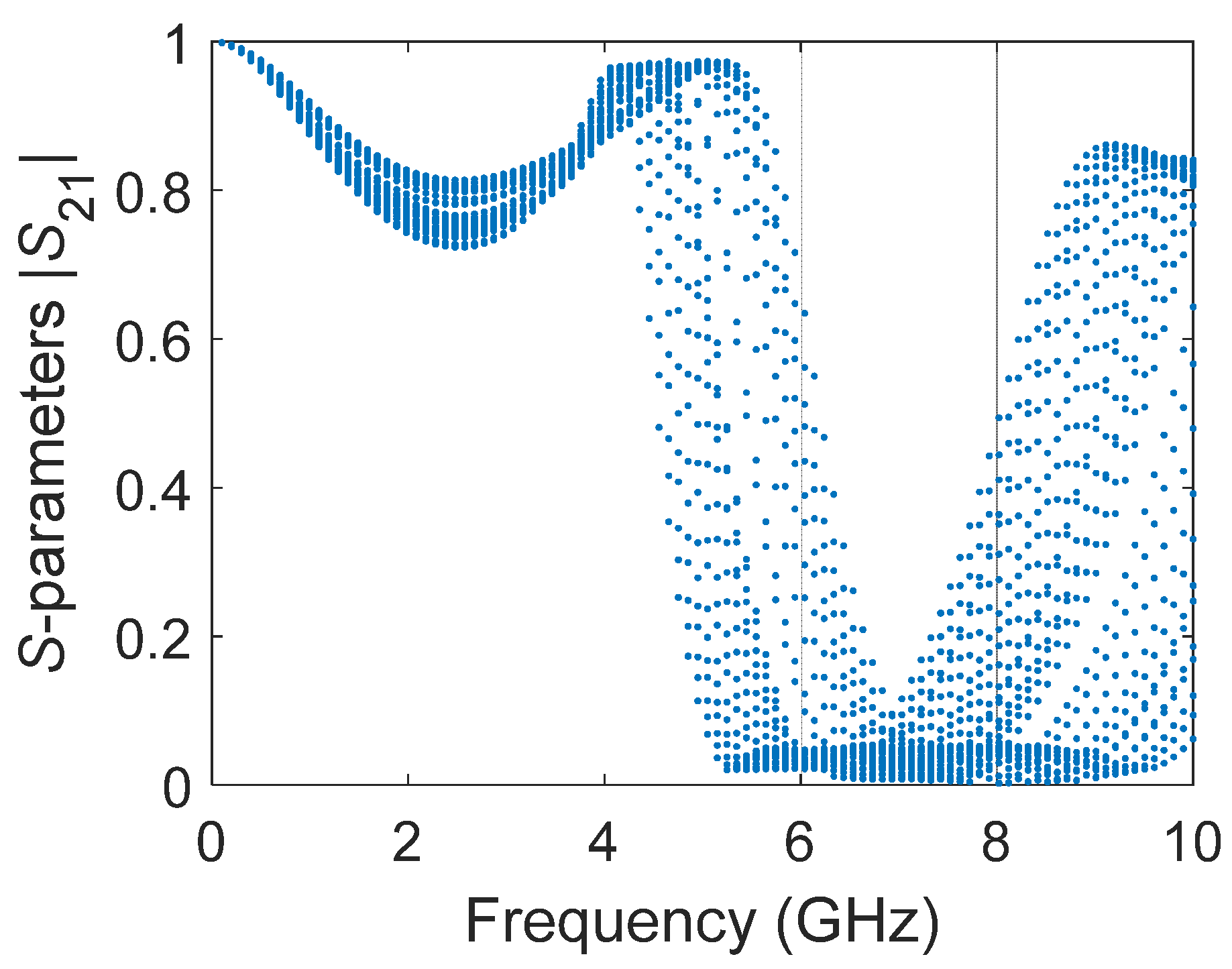
2.1. Structure Under Study

The proposed structure under study corresponds to a microstrip low-pass filter designed to operate efficiently in the microwave frequency range. Such filters are widely employed in wireless communication systems, radar front-ends, and radio frequency (RF) circuitry, where it is essential to suppress high-frequency components while maintaining low insertion loss in the passband.

The filter structure consists of a symmetric configuration of microstrip transmission lines, where the input and output ports—characterized by a 50-Ω impedance—are coupled to a wider central microstrip line [32]. This central section has a width W, is electromagnetically coupled through a separation gap S, and is terminated at both ends by open-circuited stubs of length L, which act as resonant elements. These stubs introduce frequency-selective behavior, enabling the realization of the desired low-pass response. Initial values correspond to W = 1.6406 mm, S = 3.0188 mm, and L = 4.2 mm.

The structure is implemented on a dielectric substrate with well-defined characteristics of relative permittivity ε_r = 2.2, loss tangent tan(δ) = 0.01, and includes conductor and dielectric losses. Metallic layers are composed of high-conductivity copper (σ = 5.8 × 107 S/m) with a thickness th = 15.24 μm, which ensures a realistic representation of practical losses.

From an electromagnetic standpoint, the filter operates based on distributed resonance and coupled-line principles, allowing for precise control of the cutoff frequency and stopband characteristics through geometric parameters such as widths, lengths, and gaps. These design parameters are critical and are therefore subject to optimization to meet stringent performance specifications.

Each simulation point was evaluated using COMSOL Multiphysics, with adaptive meshing and a frequency sweep from 0 to 10 GHz across 201 points, ensuring detailed characterization of the frequency response, especially in resonance regions. Input and output ports were configured using waveguide ports with impedance matching conditions to emulate real-world RF measurements.

2.2. Training Data Generation and Surrogate Modeling

This section provides not only the description of the data generation process through EM simulations but also details the preprocessing steps applied to ensure the consistency and physical reliability of the dataset.

A series of EM simulations were performed by sweeping L over a predefined range to produce corresponding frequency responses. These responses were then used to train an inverse surrogate model capable of predicting the optimal value of L given a desired frequency response. This inverse approach enables direct estimation of design parameters from performance targets, bypassing traditional iterative forward simulations and accelerating the optimization process.

To ensure representative sampling, Latin Hypercube Sampling (LHS) was employed to generate 31 design points distributed over the L range. This method guarantees that each subinterval of the parameter space is sampled uniformly, promoting broad coverage and avoiding clustering [24,33,34]. The generated values of L followed a uniform distribution across the design interval, which was defined as ±50% of its nominal value (i.e., from 2.1 mm to 6.3 mm), ensuring diverse frequency responses that span from over-damped to under-damped behaviors.

Each simulation point was evaluated using COMSOL Multiphysics, with adaptive meshing and a frequency sweep from 0 to 10 GHz across 301 points, ensuring detailed characterization of the frequency response, especially in resonance regions. Input and output ports were configured using waveguide ports with impedance matching conditions to emulate real-world RF measurements.

Prior to model training, all simulated frequency response data were normalized using min–max scaling to [0, 1] to ensure consistency across the dataset. Additionally, four data points were removed during preprocessing due to anomalous behavior. The decision to exclude these samples was based on the following criteria: (1) large deviation (>3σ) from expected trends in cutoff frequency or insertion loss, (2) abrupt discontinuities in the frequency response suggesting numerical instability in the EM simulation, and (3) lack of physical interpretability based on known microstrip filter theory. These exclusions ensured that only physically meaningful and statistically consistent data were used to train the inverse surrogate model.

To further clarify the process of generating, training, and evaluating the inverse surrogate model, we present a workflow diagram in Figure 1. The diagram provides the methodology, detailing each step from data generation to computational efficiency analysis. The workflow begins with defining the design parameter range and simulating frequency responses, followed by training an ANN to learn the inverse mapping function. The trained model is then validated against test data and applied to space mapping optimization, where it is compared with the traditional approach. Finally, the computational cost is evaluated to highlight the efficiency improvements of the proposed method.

Figure 2 shows the frequency response $\left|s_{21}\right|$ across the specified range used for data sampling during surrogate model generation. The blue dots represent training points, uniformly sampled from 0 to 10 GHz to ensure the diversity and representativeness of the dataset.

To evaluate the performance of the inverse surrogate model, four performance metrics were computed, including the mean absolute error (MAE), Maximum Absolute Relative Error (MARE), Root Mean Squared Error (RMSE), and the coefficient of determination (R²). The MAE and MARE quantify the average and maximum deviation from the target values, respectively, while the RMSE penalizes larger deviations more heavily, providing a sense of error magnitude. R² measures how well the predictions approximate the actual data distribution.

The calculated results were as follows: MAE = 0.0262, MARE = 1.99%, RMSE = 0.0315, and R² = 0.987. These values indicate that the inverse surrogate model accurately captures the system behavior with strong generalization capability and minimal error. These metrics indicate that the inverse surrogate model is highly capable of capturing the underlying system trends with minimal error, making it a reliable tool for predicting design parameters based on target performance metrics.

Figure 3 presents the training and testing errors of the generated inverse surrogate model, including the MAE and MARE values, to provide a visual perspective of model accuracy and robustness, with training and testing errors kept to a minimum, indicating efficient learning and reliable generalization.

2.3. Mathematical Formulation of the Inverse Model and Optimization Process

This section presents the mathematical foundations that support the inverse modeling and optimization strategy. The goal is to establish a functional mapping between desired circuit performance and physical design parameters.

2.3.1. Electromagnetic Modeling

The frequency response of the low-pass microstrip filter is described using the scattering parameter |S₍₂₁₎(f)|, which depends on the geometry:

S₂₁(f) = H(f; L, W, S)

where

• f ∈ [0, 10] GHz is the operating frequency;
• L, W, and S represent the stub length, the width of the center strip, and the coupling gap, respectively.

2.3.2. Inverse Modeling Using Bayesian Neural Networks

The inverse surrogate model directly maps performance metrics y (e.g., cutoff frequency or attenuation) to design parameters x = [L, W, S]^T, as follows:

x = f_BNN(y) + ε

where f_BNN is a Bayesian Neural Network, and ε follows a normal distribution ε ~ $\mathcal{N}$(0, σ²) representing uncertainty.

The model is trained to maximize the posterior probability of the weights w, given a dataset D = {(y⁽ⁱ⁾, x⁽ⁱ⁾)}, by optimizing the following:

log p(w|D) ∝ log p(D|w) + log p(w)

Bayesian Neural Networks (BNNs) estimate predictive uncertainty by modeling the weights of the network as probability distributions rather than fixed values. Specifically, a prior distribution p(w) is placed over the weights, which is updated via Bayes’ theorem into a posterior p(w|D) after observing the training data D. This probabilistic treatment enables the BNN to capture confidence intervals in the predictions, which is particularly important for inverse modeling in highly nonlinear or under-constrained design spaces. By accounting for uncertainty, the model avoids overfitting and provides more robust parameter estimates, which is crucial when a small number of high-fidelity simulations are available.

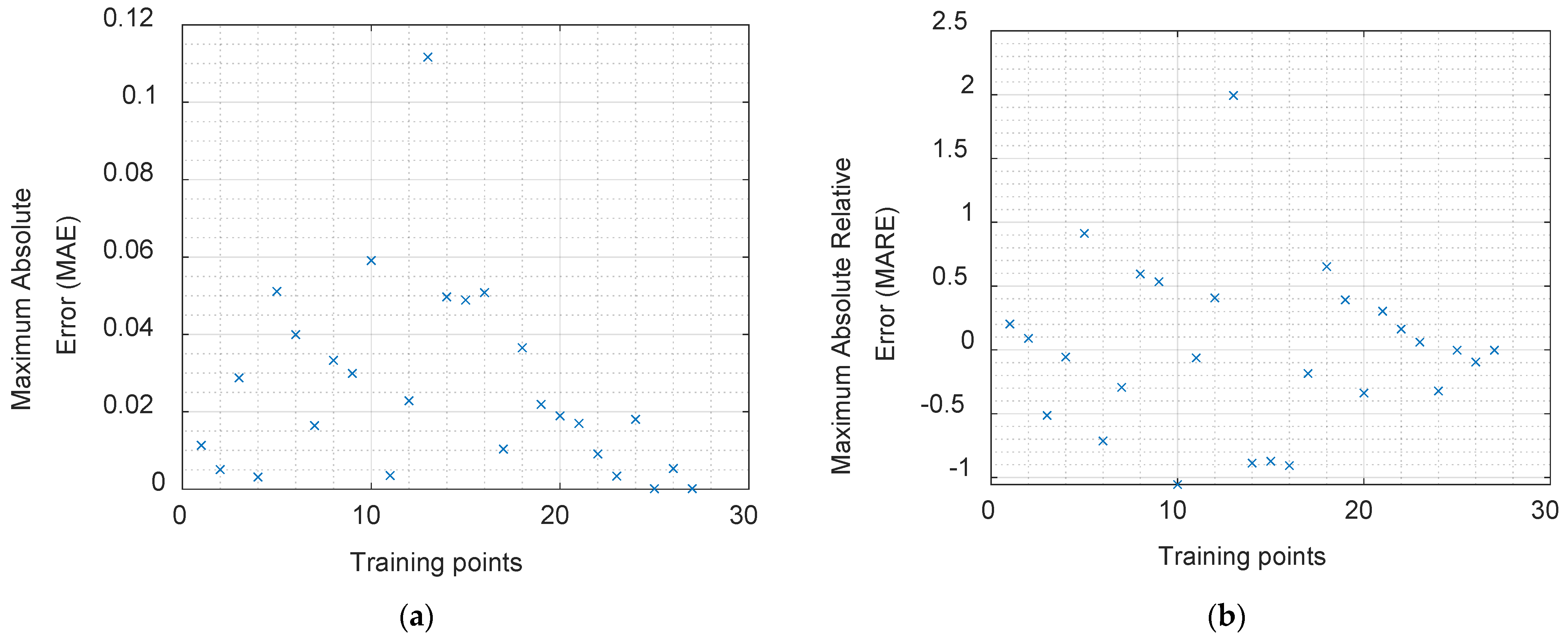
2.3.3. Accuracy Metrics

To evaluate the model’s performance, we use the following metrics:

• Mean absolute error (MAE):

  $$\mathrm{M}\mathrm{A}\mathrm{E}=(1/\mathrm{N})\sum |x_i-\widehat{x_1}|$$
• Maximum Absolute Relative Error (MARE):

  $$\mathrm{M}\mathrm{A}\mathrm{R}\mathrm{E}={\mathrm{m}\mathrm{a}\mathrm{x}}_{\mathrm{i}}\left(\right|x_{\mathrm{i}}-\widehat{x_1}|/|x_{\mathrm{i}}\left|\right)\times 100\%$$
• Root Mean Squared Error (RMSE):

  $$\mathrm{R}\mathrm{M}\mathrm{S}\mathrm{E}=\surd \left[\right(1/\mathrm{N})\sum {(x_{\mathrm{i}}-\widehat{x_1})}^2]$$
• Coefficient of determination (R²):

  $${\mathrm{R}}^2=1-[\sum {(x_{\mathrm{i}}-\widehat{x_1})}^2/\sum {(x_{\mathrm{i}}-\overline{x})}^2]$$

  where $\widehat{x_1}$ is the predicted value, x_i is the true value, and $\overline{x}$ is the mean of all x_i.

2.3.4. Optimization Strategy

The output of the BNN serves as an initial point for a trust region optimization algorithm that minimizes the error between the simulated and target frequency response:

min_X ∑ [S₂₁_sim(f_j; x) − S₂₁_target(f_j)]², for j = 1 to M

where S₂₁_sim is the high-fidelity simulation, S₂₁_target is the target response, f_j are the sampled frequency points, and M is the total number of frequency samples used in the comparison (e.g., M = 301).

3. Enhanced Convergence Analysis: A Comparative Study of Traditional Space Mapping vs. Inverse Surrogate Modeling

The traditional SM process, as introduced by Bandler et al. [4], despite being an established methodology for high-frequency circuit optimization, often involves a substantial number of iterative steps to achieve the desired design accuracy. This section presents an in-depth analysis of the results obtained from applying the classical SM process to a high-frequency circuit optimization scenario, highlighting the computational resources required and the resultant design quality.

In this work, the classical SM approach involved seven iterations of the space mapping process to converge on an optimal solution. This convergence was driven by 7 simulations of the high-fidelity model and 580 simulations of the coarse model. The significant difference in the number of simulations between the coarse and fine models emphasizes the efficiency offered by SM in leveraging the low computational cost of the coarse model while minimizing the use of computationally expensive fine model simulations.

The final parameter value of the fine model, denoted as $x_f^{\ast }$ = 6.7330, was achieved after these iterations. This parameter represents the optimal design characteristic that satisfies the performance specifications of the high-frequency circuit. The ability of the SM process to converge on this parameter with relatively few high-fidelity simulations demonstrates the effectiveness of SM in optimizing computational resources while maintaining design accuracy.

However, it is evident from the results that the traditional SM method still requires a considerable number of coarse model simulations to guide the optimization process. The 580 simulations of the coarse model reflect the iterative nature of the classical SM approach, where the coarse model is iteratively refined to align with the fine model’s behavior. This reliance on numerous coarse model simulations highlights a key limitation of the traditional SM approach specifically, the high computational burden associated with the iterative mapping and refinement process, especially for complex high-frequency circuits where the design space is highly nonlinear.

Figure 4 shows the results using the inverse surrogate model within the space mapping process. The turquoise line represents the optimal coarse model response, which is the desired target for the fine model. The red line shows the initial fine model response, while the dark blue line depicts the final fine model response after completing the SM process, demonstrating the evolution toward the target response.

Figure 4a effectively demonstrates the convergence efficiency of the space mapping process. The coarse model undergoes multiple simulations to explore the design space, while the fine model is used sparingly, ultimately minimizing the computational cost associated with high-fidelity evaluations. The figure emphasizes the iterative nature of the optimization, where each iteration refines the mapping between the coarse and fine models, gradually reducing the discrepancy between them. By achieving convergence in six iterations and using only six fine model simulations, the effectiveness of space mapping in reducing the computational overhead is clearly illustrated.

The convergence behavior observed in Figure 4a highlights both the strengths and limitations of the traditional SM approach. While SM effectively reduces the number of expensive high-fidelity simulations, the iterative nature of coarse model refinement can become less efficient in scenarios involving highly nonlinear design parameters or complex circuit behavior. This emphasizes the need for more advanced techniques to further enhance the optimization process.

Compared to traditional SM, the proposed method illustrated in Figure 4b significantly improves convergence efficiency and precision. It requires only 31 simulations of the coarse model to generate the inverse surrogate model, dramatically reducing the need for repeated high-fidelity evaluations. The final parameter value achieved by the proposed model was 6.6709, illustrating its high precision and reduced computational cost. By eliminating repetitive iterative cycles, this method reduces the computational overhead and mitigates issues related to convergence to suboptimal solutions, making it particularly well suited for rapid and accurate high-frequency circuit optimization.

Sensitivity to the Number of Training Samples

To analyze the effect of the training set size on the performance of the inverse model, we conducted a sensitivity study using subsets of the original 31-point dataset generated by Latin Hypercube Sampling. Specifically, models were trained using 10, 20, 25, and all 31 design points. The results indicate a clear improvement in accuracy with increased data size, as measured by the mean absolute error (MAE). However, the marginal gain beyond 25 samples is relatively small, suggesting that the model achieves a good balance between precision and data efficiency. This is particularly relevant in high-fidelity EM design, where the simulation cost is significant.

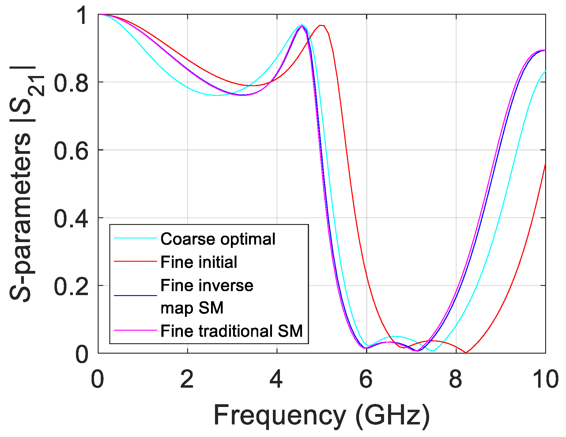
4. Comparison of Results

4.1. Accuracy and Convergence Analysis

The superior performance of the inverse surrogate model stems from two key factors: (a) Direct inverse mapping eliminates iterative coarse model refinements, accelerating convergence. (b) BNN uncertainty quantification reduces error propagation, leading to more stable and reliable parameter predictions [35]. Unlike traditional space mapping, which relies on iterative forward evaluations to refine design parameters, the inverse surrogate model provides a direct mapping between performance specifications and optimal design variables. This not only improves computational efficiency but also reduces sensitivity to local minima, ensuring a more robust optimization process.

The final optimization results show that both traditional SM and the inverse surrogate modeling approach successfully achieve the desired output values. However, the inverse surrogate model produces results closer to the target objectives with fewer iterations, demonstrating its improved accuracy. Figure 5 illustrates the optimized responses obtained through both methods. The turquoise line represents the ideal coarse model response, while the red and blue lines depict the initial and final fine model responses, respectively. The magenta line represents the final response using traditional SM. As shown, the inverse surrogate model exhibits a smoother convergence toward the target, confirming its enhanced precision.

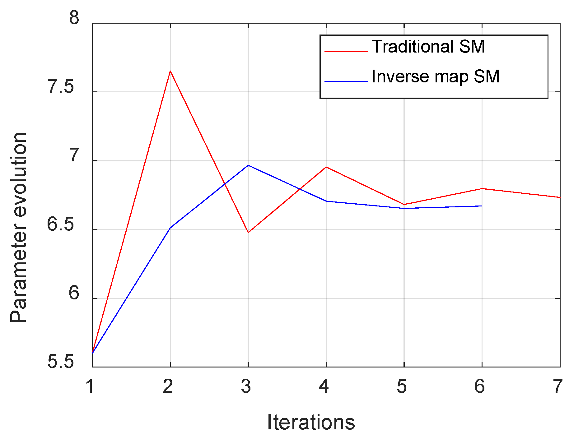
4.2. Optimization Parameter Evolution

Another critical advantage of inverse surrogate modeling is its ability to maintain a smoother evolution of optimization parameters. Traditional SM often exhibits large fluctuations and irregularities, requiring additional iterations to refine parameter values. Figure 6 compares the parameter evolution trajectories for both methods. The inverse surrogate model maintains a more stable progression, while the traditional SM method undergoes significant oscillations before converging. This demonstrates that inverse mapping leads to a more robust and predictable optimization process.

4.3. Computational Efficiency and Burden Reduction

A major advantage of inverse surrogate modeling is its ability to significantly reduce the computational costs. In traditional SM, the coarse model is iteratively refined across multiple iterations, resulting in an increasing number of simulations. In contrast, the inverse surrogate model requires a fixed number of coarse model evaluations before transitioning directly to the optimization phase. Figure 7 highlights the computational differences between the two approaches. The traditional SM method requires 580 coarse model simulations and 7 fine model simulations for convergence, whereas the inverse surrogate model requires only 31 coarse simulations and 6 fine simulations. This substantial reduction in required simulations makes the inverse surrogate modeling approach more computationally efficient and scalable for large-scale circuit optimization.

4.4. Comparative Discussion

Compared to traditional models such as Gaussian Process Regression (GPR) and Support Vector Regression (SVR), Bayesian Neural Networks (BNNs) offer the advantage of predictive uncertainty quantification, which is especially valuable in inverse design problems involving nonlinearity and limited data. While a complete numerical benchmark is beyond the scope of this work, we have included a qualitative comparison to highlight the distinctive features of the proposed method. A more exhaustive comparative analysis will be explored in future work.

5. Conclusions

The proposed inverse surrogate modeling approach significantly enhances the efficiency of high-frequency circuit optimization by leveraging machine learning for direct parameter prediction. This method circumvents the iterative refinements required in SM, leading to faster convergence, reduced computational demands, and improved robustness against nonlinearities. Unlike conventional SM, which relies on multiple iterative fine model evaluations, the proposed approach eliminates these redundant refinements by directly mapping performance specifications to design parameters using BNNs.

The results demonstrate that the proposed method achieves over 80% reduction in fine model evaluations while maintaining high accuracy: MAE: 0.0262, MARE: 1.99% (Figure 3). The faster convergence rate (Figure 5 and Figure 6) and smoother optimization trajectory (Figure 6) further validate the robustness of the approach. Additionally, Figure 7 highlights the computational efficiency improvement, demonstrating that the inverse surrogate model requires only 31 coarse model simulations compared to 580 in traditional SM.

These findings illustrate that inverse surrogate modeling is a computationally efficient, accurate, and scalable alternative to conventional SM techniques, making it highly suitable for practical applications in RF and microwave circuit optimization. The substantial reduction in computational costs and smoother parameter evolution make this approach particularly valuable for applications requiring rapid prototyping and precise optimization, underscoring its potential impact in high-frequency system design.

While this study focused on a microstrip low-pass filter as a representative use case, the proposed inverse surrogate modeling approach is designed to be broadly applicable to other high-frequency circuit topologies, including band-pass filters, impedance matching networks, and resonant structures. The methodology—based on physics-informed sampling, Bayesian Neural Networks, and surrogate optimization—is not limited to a specific topology or response type. Nonetheless, we acknowledge that further validation across a wider range of circuit types is essential to fully assess model robustness. As part of future work, we plan to apply the proposed framework to additional scenarios involving multi-parameter models, distributed-element filters, and active circuit components, to systematically evaluate its generalization capability across diverse microwave design problems.

Limitations and Future Work

While the proposed inverse surrogate modeling framework demonstrates strong predictive capabilities in simulation environments, we acknowledge that no experimental validation was conducted in this study. In future work, we plan to fabricate and measure physical prototypes of the optimized circuits to assess the accuracy of the proposed method in practical scenarios and confirm the simulation-based findings.

References

1. Pietrenko-Dąbrowska, A.; Koziel, S.; Raef, A.G. Reduced-Cost Optimization-Based Miniaturization of Microwave Passives by Multi-Resolution EM Simulations for Internet of Things and Space-Limited Applications. Electronics 2022, 11, 4094. [Google Scholar] [CrossRef]
2. Pissoort, D. Bayesian Optimization for Microwave Devices Using Deep Gaussian Processes. IEEE Trans. Microw. Theory Tech. 2023, 71, 2396–2408. [Google Scholar] [CrossRef]
3. Liu, Z.; Zhao, M.; Wang, J.; Zhang, Y. AI-Driven Multiobjective Optimization of Antennas Using Surrogate Models and Multi-Fidelity EM Analysis. Sci. Rep. 2025, 15, 21776. [Google Scholar] [CrossRef]
4. Bandler, J.W.; Biernacki, R.M.; Chen, S.H.; Grobelny, P.A.; Hemmers, R.H. Space mapping technique for electromagnetic optimization. IEEE Trans. Microw. Theory Tech. 1994, 42, 2536–2544. [Google Scholar] [CrossRef]
5. Nguyen, T.; Lu, L.; Tanaka, M. Global Parameter Tuning of Microwave Filters via AI-Driven Optimization and EM Co-Simulation. Sci. Rep. 2025, 15, 21776. [Google Scholar] [CrossRef]
6. Bakr, M.H.; Bandler, J.W.; Georgieva, N.; Madsen, K. A hybrid aggressive space-mapping algorithm for EM optimization. IEEE Trans. Microw. Theory Tech. 1999, 47, 2440–2449. [Google Scholar] [CrossRef]
7. Simpson, T.W.; Peplinski, J.; Koch, P.N.; Allen, J.K. Metamodels for computer-based engineering design: Survey and recommendations. Eng. Comput. 2001, 17, 129–150. [Google Scholar] [CrossRef]
8. Queipo, N.V.; Haftka, R.T.; Shyy, W.; Goel, T.; Vaidyanathan, R.; Tucker, P.K. Surrogate-based analysis and optimization. Prog. Aerosp. Sci. 2005, 41, 1–28. [Google Scholar] [CrossRef]
9. Bandler, J.W.; Cheng, Q.S.; Dakroury, S.A.; Mohamed, A.S.; Bakr, M.H.; Madsen, K.; Sondergaard, J. Space mapping: The state of the art. IEEE Trans. Microw. Theory Tech. 2004, 52, 337–361. [Google Scholar] [CrossRef]
10. Koziel, S.; Bandler, J.W.; Madsen, K. Space mapping optimization algorithms for engineering design. In Proceedings of the 2006 IEEE MTT-S International Microwave Symposium Digest, San Francisco, CA, USA, 11–16 June 2006; pp. 1601–1604. [Google Scholar] [CrossRef]
11. Bandler, J.W.; Cheng, Q.S.; Nikolova, N.K.; Ismail, M.A. Implicit space mapping optimization exploiting preassigned parameters. IEEE Trans. Microw. Theory Tech. 2004, 52, 378–385. [Google Scholar] [CrossRef]
12. Koziel, S.; Bandler, J.W. Space-Mapping Optimization With Adaptive Surrogate Model. IEEE Trans. Microw. Theory Tech. 2007, 55, 541–547. [Google Scholar] [CrossRef]
13. Koziel, S.; Bandler, J.W.; Madsen, K. Enhanced surrogate models for statistical design exploiting space mapping technology. In Proceedings of the 2005 IEEE MTT-S International Microwave Symposium Digest, Long Beach, CA, USA, 17 June 2005; pp. 1609–1612. [Google Scholar] [CrossRef]
14. Amari, S.; LeDrew, C.; Menzel, W. Space-mapping optimization of planar coupled-resonator microwave filters. IEEE Trans. Microw. Theory Tech. 2006, 54, 2153–2159. [Google Scholar] [CrossRef]
15. Choi, H.-S.; Kim, D.H.; Park, I.H.; Hahn, S.Y. A new design technique of magnetic systems using space mapping algorithm. IEEE Trans. Magn. 2001, 37, 3627–3630. [Google Scholar] [CrossRef]
16. Redhe, M.; Nilsson, L. Using space mapping and surrogate models to optimize vehicle crashworthiness design. In Proceedings of the 9th AIAA/ISSMO Symposium on Multidisciplinary Analysis and Optimization, Atlanta, GA, USA, 2–6 September 2002. [Google Scholar] [CrossRef]
17. Rayas-Sanchez, J.E.; Lara-Rojo, F.; Martinez-Guerrero, E. A linear inverse space-mapping (LISM) algorithm to design linear and nonlinear RF and microwave circuits. IEEE Trans. Microw. Theory Tech. 2005, 53, 960–968. [Google Scholar] [CrossRef]
18. Zhang, L.; Xu, J.; Yagoub, M.C.E.; Ding, R.; Zhang, Q.-J. Efficient analytical formulation and sensitivity analysis of neuro-space mapping for nonlinear microwave device modeling. IEEE Trans. Microw. Theory Tech. 2005, 53, 2752–2767. [Google Scholar] [CrossRef]
19. Zhang, Q.-J.; Gupta, K.C.; Devabhaktuni, V.K. Artificial neural networks for RF and microwave design—from theory to practice. IEEE Trans. Microw. Theory Tech. 2003, 51, 1339–1350. [Google Scholar] [CrossRef]
20. Rayas-Sanchez, J.E. EM-based optimization of microwave circuits using artificial neural networks: The state-of-the-art. IEEE Trans. Microw. Theory Tech. 2004, 52, 420–435. [Google Scholar] [CrossRef]
21. Dávalos-Guzmán, J.; Chavez-Hurtado, J.L.; Brito-Brito, Z. Neural Network Learning Techniques Comparison for a Multiphysics Second Order Low-Pass Filter. In Proceedings of the 2023 IEEE MTT-S Latin America Microwave Conference (LAMC), San José, Costa Rica, 6–8 December 2023; pp. 102–104. [Google Scholar] [CrossRef]
22. Rayas-Sanchez, J.E.; Lara-Rojo, F.; Martinez-Guerrero, E. A linear inverse space mapping algorithm for microwave design in the frequency and transient domains. In Proceedings of the 2004 IEEE MTT-S International Microwave Symposium Digest (IEEE Cat. No.04CH37535), Fort Worth, TX, USA, 6–11 June 2004; Volume 3, pp. 1847–1850. [Google Scholar] [CrossRef]
23. Koziel, S.; Yang, X.-S.; Zhang, Q.-J. Simulation-Driven Design Optimization and Modeling for Microwave Engineering; Imperial College Press: London, UK, 2013. [Google Scholar]
24. Koziel, S.; Leifsson, L. Surrogate-Based Modeling and Optimization: Applications in Engineering, 1st ed.; Springer: New York, NY, USA, 2013. [Google Scholar] [CrossRef]
25. Yu, Y.; Zhang, Z.; Cheng, Q.S.; Liu, B.; Wang, Y.; Guo, C.; Ye, T.T. State-of-the-Art: AI-Assisted Surrogate Modeling and Optimization for Microwave Filters. IEEE Trans. Microw. Theory Tech. 2022, 70, 4635–4651. [Google Scholar] [CrossRef]
26. Rayas-Sánchez, J.E.; Koziel, S.; Bandler, J.W. Advanced RF and Microwave Design Optimization: A Journey and a Vision of Future Trends. IEEE J. Microw. 2021, 1, 481–493. [Google Scholar] [CrossRef]
27. Sharifuzzaman, S.A.S.M.; Tanveer, J.; Chen, Y.; Chan, J.H.; Kim, H.S.; Kallu, K.D.; Ahmed, S. Bayes R-CNN: An Uncertainty-Aware Bayesian Approach to Object Detection in Remote Sensing Imagery for Enhanced Scene Interpretation. Remote Sens. 2024, 16, 2405. [Google Scholar] [CrossRef]
28. Browne, J. 2025’s Top Trends: Artificial Intelligence and Machine Learning Bring Smarts to RF Systems. Microwaves & RF, 26 November 2024. [Google Scholar]
29. Liang, J.; Yu, Z.L.; Gu, Z.; Li, Y. Electromagnetic Source Imaging With a Combination of Sparse Bayesian Learning and Deep Neural Network. IEEE Trans. Neural Syst. Rehabil. Eng. 2023, 31, 2338–2348. [Google Scholar] [CrossRef]
30. Koziel, S.; Pietrenko-Dabrowska, A. Optimization of microwave components using machine learning and rapid sensitivity analysis. Sci. Rep. 2024, 14, 31265. [Google Scholar] [CrossRef]
31. Davalos-Guzman, J.; Chavez-Hurtado, J.L.; Brito-Brito, Z. Integrative BNN-LHS Surrogate Modeling and Thermo-Mechanical-EM Analysis for Enhanced Characterization of High-Frequency Low-Pass Filters in COMSOL. Micromachines 2024, 15, 647. [Google Scholar] [CrossRef]
32. Rayas-Sánchez, J.E.; Brito-Brito, Z.; Cervantes-González, J.C.; López, C.A. Systematic configuration of coarsely discretized 3D EM solvers for reliable and fast simulation of high-frequency planar structures. In Proceedings of the 2013 IEEE 4th Latin American Symposium on Circuits and Systems (LASCAS), Cusco, Peru, 27 February 2013; pp. 1–4. [Google Scholar] [CrossRef]
33. McKay, M.D.; Beckman, R.J.; Conover, W.J. A Comparison of Three Methods for Selecting Values of Input Variables in the Analysis of Output from a Computer Code. Technometrics 1979, 21, 239–245. [Google Scholar] [CrossRef]
34. Dávalos-Guzmán, J.; Chavez-Hurtado, J.L.; Brito-Brito, Z.; Ortstein, K. Space Sampling Techniques Comparison for a Synthetic Low-Pass Filter Bayesian Neural Network. In Proceedings of the 2023 IEEE MTT-S Latin America Microwave Conference (LAMC), San José, Costa Rica, 6–8 December 2023; pp. 109–112. [Google Scholar] [CrossRef]
35. De Witte, D.; Qing, J.; Couckuyt, I.; Dhaene, T.; Vande Ginste, D.; Spina, D. A Robust Bayesian Optimization Framework for Microwave Circuit Design under Uncertainty. Electronics 2022, 11, 2267. [Google Scholar] [CrossRef]
Figure 1. Workflow for inverse surrogate model training and evaluation.
Electronics 14 03097 g001
Figure 2. Frequency response points for surrogate model training.
Electronics 14 03097 g002
Figure 3. Training error analysis of the inverse surrogate model showing both training and testing errors: MAE (a) and MARE (b), which confirm the stability and predictive accuracy of the model.
Electronics 14 03097 g003
Figure 4. Convergence results for (a) traditional space mapping and (b) inverse map surrogate space mapping.
Electronics 14 03097 g004
Figure 5. Comparison of optimization results: the inverse surrogate model converges faster and more accurately to the target response compared to traditional space mapping.
Electronics 14 03097 g005
Figure 6. Comparative evolution of optimization parameters using traditional SM method vs. proposed inverse map surrogate model.
Electronics 14 03097 g006
Figure 7. Coarse model evaluations in traditional SM vs. inverse map surrogate model approach. This figure shows the number of coarse model evaluations required to reach the optimal solution during the space mapping process.
Electronics 14 03097 g007
Disclaimer/Publisher’s Note: The statements, opinions and data contained in all publications are solely those of the individual author(s) and contributor(s) and not of MDPI and/or the editor(s). MDPI and/or the editor(s) disclaim responsibility for any injury to people or property resulting from any ideas, methods, instructions or products referred to in the content.