BCA-MVSNet: Integrating BIFPN and CA for Enhanced Detail Texture in Multi-View Stereo Reconstruction

Abstract

The 3D point cloud generated by MVSNet has good scene integrity but lacks sensitivity to details, causing holes and non-dense areas in flat and weak-texture regions. To address this problem and enhance the point cloud information of weak-texture areas, the BCA-MVSNet network is proposed in this paper. The network integrates the Bidirectional Feature Pyramid Network (BIFPN) into the feature processing of the MVSNet backbone network to accurately extract the features of weak-texture regions. In the feature map fusion stage, the Coordinate Attention (CA) mechanism is introduced into 3DU-Net to obtain the position information on the channel dimension related to the direction, improve the detail feature extraction, optimize the depth map and improve the depth accuracy. The experimental results show that BCA-MVSNet not only improves the accuracy of detail texture reconstruction, but also effectively controls the computational overhead. In the DTU dataset, the Overall and Comp metrics of BCA-MVSNet are reduced by 10.2% and 2.6%, respectively; in the Tanksand Temples dataset, the Mean metrics of the eight scenarios are improved by 6.51%. Three scenes are shot by binocular camera, and the reconstruction quality is excellent in the weak-texture area by combining the camera parameters and the BCA-MVSNet model.

1. Introduction

With the country’s investment in the field of computer vision, visual 3D reconstruction has become a key technology [1]. Monocular cameras achieve good reconstruction results through the classic Structure from Motion (SfM) method [2], but suffer from poor real-time performance and low fault tolerance. The binocular camera [3,4] uses the parallax of the left and right cameras [5] to accurately reconstruct the spatial information of three-dimensional objects by imitating the structure of human eyes. After reasonable calibration, binocular cameras can complete high-precision 3D reconstruction by capturing two images [6], offering superior real-time performance and accuracy, thus becoming a primary tool for modern 3D reconstruction. Image depth estimation is a key step in 3D reconstruction. Traditional methods such as PMVS [7] and Colmap [8] calculate the depth of each pixel by extracting manual features and using geometric methods. However, due to the limitations of manual features, these methods often fail to effectively improve the integrity of the reconstruction model in weak-texture areas or under strong lighting conditions. The introduction of convolutional neural networks [9,10,11,12] has promoted the progress in the field of computer vision, especially in multi-view stereo technology based on deep learning, which has made remarkable breakthroughs [13,14,15].

Multi-view stereo (MVS) [16,17] is similar to the structure recovery method (SFM) of monocular cameras, which relies on camera shooting and combines camera parameters to reconstruct, but the point cloud generated by MVS is more dense. However, MVS performs poorly in weak-texture regions and is susceptible to external interference. 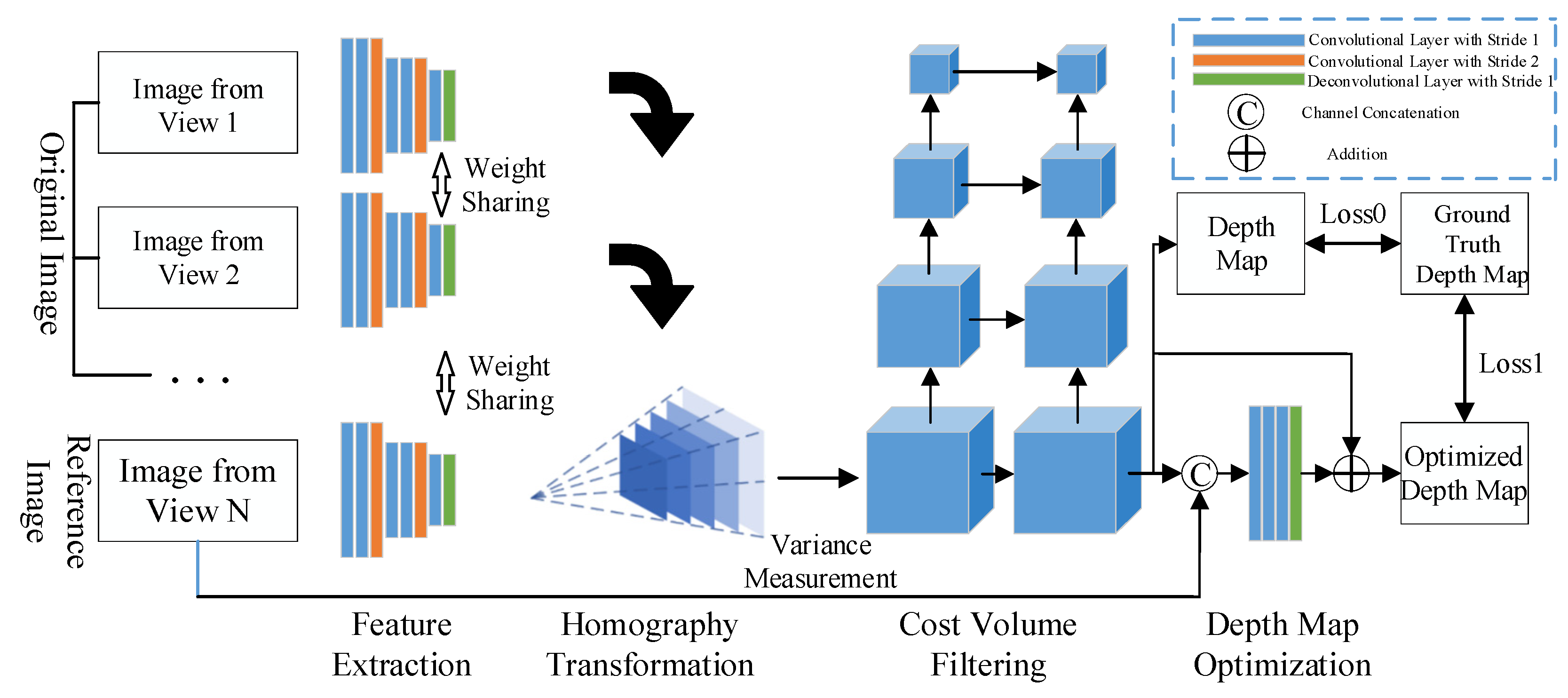In order to solve these problems, researchers introduced deep learning into MVS [18]. Yao et al. [19] proposed an epoch-making MVSNet network, which includes four parts: feature extraction, homography transformation, cost volume filtering and depth map optimization. Subsequently, aiming at the memory consumption of MVSNet, Yao et al. proposed R-MVSNet to solve the memory bottleneck in network training. Compared with the MVSNet network, the R-MVSNet network [20] is equipped with a gated loop and a recurrent neural network, and the GPU occupancy can be reduced by about 200%.

From the point of view of the balance between feature fusion and accuracy, the existing methods have significant performance trade-offs. Fast-MVSNet proposed by Yu [21] et al. improves the reconstruction speed by optimizing the learning ability of the cost body, but sacrifices the final accuracy for the pursuit of efficiency. Although Ding [22] et al.’s TransMVSNet introduces the Transformer mechanism to significantly improve the reconstruction accuracy, the reconstruction efficiency is greatly reduced due to the aggregation of long-distance context information. Similarly, although Chen [23] et al.’s method takes into account both local and global information, its real-time performance is not good. Ge [24] et al.’s method of combining TSDF and SDF improves the geometric accuracy, but the training time is significantly increased due to the progressive training strategy. This imbalance between accuracy and efficiency has become a key bottleneck restricting the practical application of MVS method.

In the feature processing of complex scenes, the existing methods are not robust to weak textures, illumination changes and occlusions. Ye [25] et al.’s method based on a feature pyramid network tries to solve the problem of weak textures through multi-scale fusion, but it leads to the decline of depth map accuracy; Zhang [26] et al.’s Attention-aware 3DU-Net has limited reconstruction effect due to insufficient consideration of channel relevance; Yu [27] et al.’s independent self-attention mechanism has poor performance in point cloud accuracy in weak-texture areas; and Li [28] et al.’s HDCMVSNet has difficulty in solving detail blur caused by occlusion and uneven brightness in remote sensing scenes. It is particularly noteworthy that Cas-MVSNet, as a representative method to solve the depth map in stages, reduces the memory consumption through hierarchical fusion, but in the scene with lack of texture or large illumination changes, the reconstruction integrity decreases significantly, it is difficult to capture the details and geometric structure of the scene and there is no point cloud in the local area.

In terms of the adaptability and efficiency of the model design, the architectural defects of the existing methods further limit the performance improvement. Wang [29] et al. introduced the traditional Patchmatch algorithm to deep learning, which is superior in integrity, but slightly inferior in accuracy; and the remote grouping attention mechanism proposed by Yang [30] leads to a cubic increase in GPU memory demand due to voxelization processing. The generalizability of the multi-scale feature extraction module by Zhu [31] et al. is insufficient, and faces difficulty adapting to diverse scenes. The core of these problems lies in the lack of sensitivity to detailed information in the feature extraction stage, the lack of dynamic adaptation to multi-view geometric consistency in the feature fusion process and the failure to effectively establish the association between channels and spatial information in the cost volume regularization stage.

In order to overcome these limitations, BCA-MVSNet (Bidirectional Feature Pyramid Network and Coordinate Attention mechanism-enhanced MVSNet) is proposed in this paper. High-precision reconstruction of complex scenes is achieved through innovative architecture design. In the feature extraction stage, the Bidirectional Feature Pyramid Network (BIFPN) is introduced, and the number of convolution layers is increased to retain the feature information of weak-texture regions, which solves the problem of detail loss in traditional feature fusion. The coordinate attention mechanism (CA) is introduced in the cost volume regularization stage to strengthen the correlation between channels and spatial information, improve the model’s ability to perceive the spatial location accuracy of unstructured weak-texture large-scale scenes and enhance the model’s generalizability to different scenes. Through the collaborative design of BIFPN and CA, BCA-MVSNet effectively makes up for the shortcomings of CAS-MVSNet in the reconstruction of weak-texture regions, and provides a new scheme for MVS matching that takes into account the accuracy, efficiency and scene adaptability.

2. Theory of Multi-View Stereo Reconstruction

2.1. Multi-View Stereo Reconstruction

In this study, a binocular reconstruction method based on two left and right views was used. By fixing the position of the binocular camera, the method monitors the local area of the infrastructure project in real time, transmits the image to the computer terminal and realizes 3D reconstruction. However, there are some limitations in binocular 3D reconstruction based on only two views. The images captured by the left and right cameras only cover their visible areas, resulting in a limited field of view, and the reconstruction effect can only generate a 3D model between the camera and the scene, but cannot present a 360° panoramic 3D model. For reconstruction tasks involving only local areas, this method can complete the reconstruction efficiently and accurately. However, when 360° panoramic reconstruction is required, a large number of 2D images must be captured, and there must be a high degree of overlap between adjacent images. This idea is similar to the MVS algorithm. This is the idea of the MVS [32] algorithm in 3D reconstruction, as shown in Figure 1. The MVS algorithm, like the binocular reconstruction idea using two images, relies on the stereovision between adjacent images.

When detecting feature points in 2D images, the MVS algorithm still uses methods such as SIFT and SURF. It then performs registration between each pair of images to generate disparity maps, and finally creates a relatively dense 3D point cloud, which is one of the differences between this method and SfM sparse point cloud reconstruction. Currently, the MVS algorithm and its principles have been fully encapsulated in the OpenMVS open-source library, facilitating use by subsequent researchers.

With the increasing application of deep learning in various fields, Yao et al. [19] began to apply powerful deep learning neural networks to the MVS framework and ultimately proposed the MVSNet network. MVSNet captures multi-view images by surrounding the main subject from multiple perspectives, then performs operations such as feature extraction, homography transformation and cost volume regularization to finally obtain the depth map of a primary view. Once the depth map is obtained, the network completes its task. To further generate a 3D point cloud, post-processing of the depth map is required.

2.2. MVSNet

The network diagram of MVSNet is shown in Figure 2.

As can be seen from Figure 2, MVSNet is able to capture multi-scale information during the depth map solving process, thereby enhancing the richness of image representation and providing a more accurate foundation for subsequent depth estimation. Secondly, MVSNet aligns images from different viewpoints to a unified direction through homography transformation, optimizing the processing of target position information between different images and providing convenient conditions for constructing the cost volume. The 3D cost volume is shown in Figure 3.

Finally, the MVSNet network estimates the depth of each pixel through a well-performing probability volume. To further capture detail texture information at different levels, the Cas-MVSNet [33] network makes modifications in some areas compared to MVSNet to reduce memory consumption and improve depth map accuracy. The specific changes are as follows: Cas-MVSNet improves image feature extraction by replacing the 8-layer convolutional neural network in the feature extraction part of MVSNet with a Feature Pyramid Network (FPN). Unlike MVSNet, it does not directly fuse feature maps from different viewpoints. Instead, it performs homography transformation and cost volume regularization separately based on the output resolutions of the FPN, ultimately generating depth maps at each resolution. The depth maps at each resolution are transmitted to the feature extraction module of the next layer as reference guidance for depth sampling. After multiple cycles of merging, a depth map with the same size as the input image is finally generated.

In this paper, we use the binocular camera to shoot the outdoor scene to be reconstructed, and then use the precise left and right segmentation algorithm to achieve the effect of MVS multi-view image.

3. BCA-MVSNet with Strong Feature Extraction and Detail Texture Information

3.1. BCA-MVSNet Network Framework

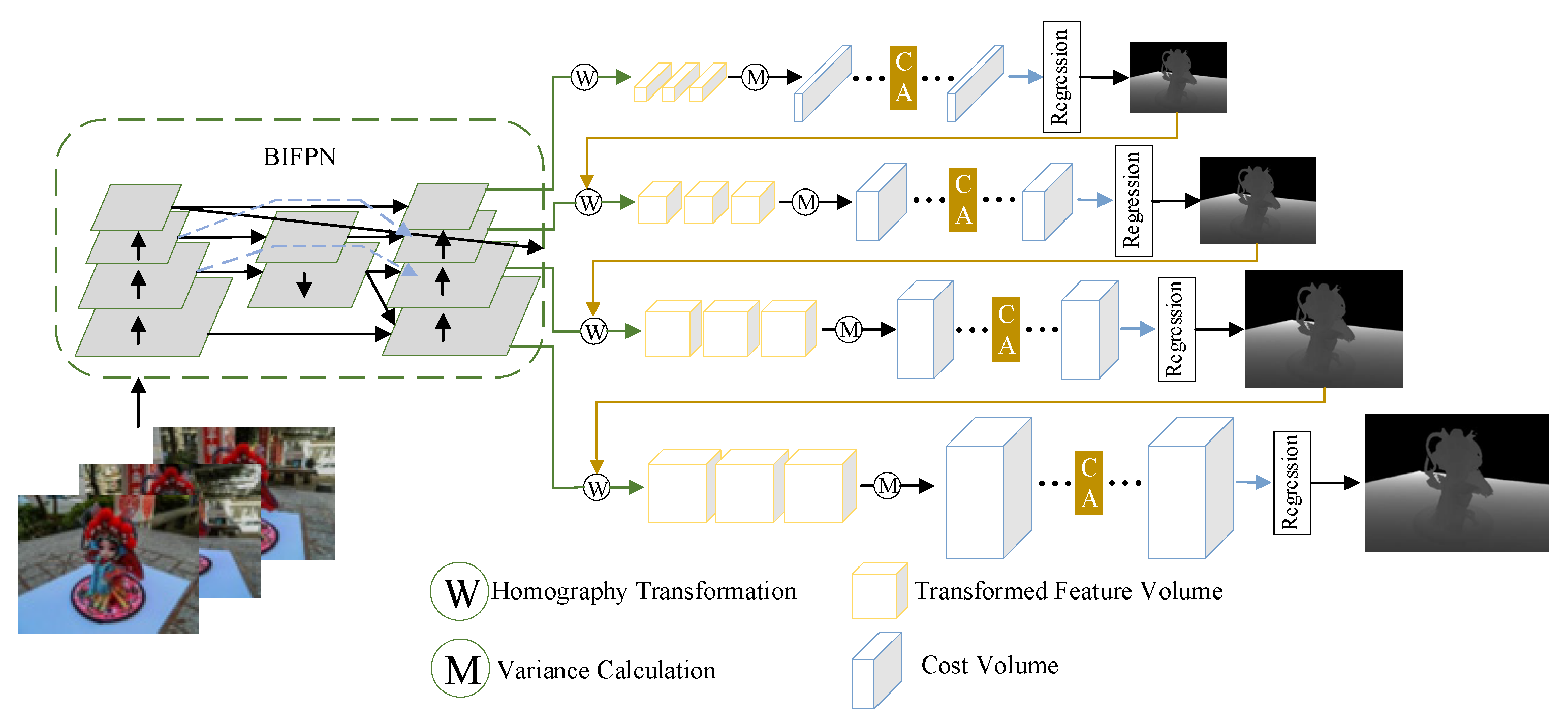
To achieve strong feature extraction and enhance point cloud information in weak-texture regions, this paper designs the BCA-MVSNet network. The overall structure and workflow of the BCA-MVSNet network remain consistent with those of Cas-MVSNet, and its improved network structure is shown in Figure 4.

BIFPN effectively solves the global consistency problem of multi-scale and multi-view features, and provides reliable feature inputs for CA. CA focuses on the extraction of local key features, and improves the overall performance by strengthening the feature fusion efficiency of BIFPN, thus forming a closed loop of global calibration–local enhancement. This method can not only ensure the structural integrity of the whole reconstruction, but also improve the reconstruction accuracy of the detail texture in complex scenes. In contrast, HRNet preserves details through parallel multi-resolution branches, but it cannot effectively adapt to the dynamic characteristics of different view-feature-important changes with the pose in MVS due to the lack of dynamic weight adjustment between branches.

When solving the depth map of the reference image, the BCA-MVSNet network goes through the following four steps:

(1) Feature Extraction

In this paper, four images are selected as the input, one of which is the reference image and the others are adjacent source images, and five feature maps are extracted. The 8-layer CNN network used by MVSNet has the problem of insufficient information exchange, which leads to the loss of underlying details. Different from MVSNet, the BIFPN structure can not only focus on strong texture regions, but also effectively extract weak-texture regions by fusing different levels of information. BCA-MVSNet adds a fine texture-detection layer at the bottom of the flat area, which is dedicated to extracting the details of the weak-texture area. Finally, the high-quality feature information of all regions is retained through feature map fusion.

(2) Homography Transformation

After feature extraction in BCA-MVSNet, the three resulting feature maps may exhibit non-coplanar characteristics due to viewpoint discrepancies. Through homography transformation, all source-image feature maps are aligned with the reference image’s coordinate system and projected into the reference camera’s stereo space. With five input images during feature extraction, homography transformation yields five feature volumes.

(3) Cost Volume Regularization

BCA-MVSNet deduces the depth map and constructs the cost volume by referring to the cone principle of the camera. In this link, the convolution kernel itself is three-dimensional, and all dimensions can be entered by it when it moves, which makes higher requirements for the two location factors of space and channel. To enrich the detail and coverage of the final probability volume from the 3D U-Net, a CA mechanism is added to the original Cas-MVSNet’s 3D U-Net. This enhancement maintains network flexibility and lightness while improving the extraction and learning of spatial and directional features, ensuring the accuracy of the probability volume.

(4) Depth Map Generation

The initial depth map is directly inferred from the probability volume. Thanks to the improvements made to Cas-MVSNet in this study, the depth map quality is significantly more accurate. However, since the reference image contains boundary information, it is used to refine the initial depth map, enhancing its representational accuracy. In the final stage of BCA-MVSNet, an end-to-end residual network is employed: the reference image is resized to match the initial depth map, and the two are combined into a 4-channel feature map. This undergoes 11 layers of 2D convolution with 32 channels, producing a single-channel-refined depth map.

3.2. BIFPN with Feature Extraction Module of a Fine Detection Layer

When using a binocular camera to derive depth maps via MVSNet in this paper, the improvements to the feature extraction module primarily involve replacing the convolutional neural network for feature extraction with BIFPN [34] and increasing the number of convolutional layers to ensure that feature information in weak-texture regions is not lost and higher-order features are extracted.

Through bidirectional cross-scale connection and dynamic weight mechanism, BIFPN can adaptively enhance the features of the same spatial point in different views, while suppressing noise interference, effectively solve the problems of feature scale mismatch and cross-view fusion ambiguity in multi-view scenes of a traditional Feature Pyramid Network (FPN) [35] and improve the geometric accuracy of feature matching.

In the networks that rely on MVSNet improvement, such as CasMVSNet and TransMVSNet, the FPN is used in the feature extraction stage. Unlike traditional algorithms such as SIFT and SURF, FPN is widely adopted by fusing high-resolution and high-semantic features. In this paper, when reconstructing the scene in the weak-texture area, while taking advantage of the convenience brought by FPN, we also perceive that when the input image has a weak-texture area where it is difficult to detect feature points in a large area, the disadvantage of FPN that it only exists in the top-down structure will lead to the fact that the information existing in the lower layer will not be transmitted to the last layer. And that fusion between high-level and low-level feature is also very inefficient. The structure block diagram of BIFPN is shown in Figure 5:

As shown in Figure 5, after designating a reference image and adding four source images as input, the feature extraction network no longer follows the FPN process that fails to fully utilize feature information. First, in the structural design of BIFPN, removing the single-ended input nodes on the upper and lower sides reduces the overall algorithm’s redundancy. Second, due to the existence of skip connections in BIFPN, it fuses more features through a combination of skip connection mechanisms and weighted fusion between original multi-scale feature maps and input feature maps at the same level, with only a slight increase in the number of parameters. Finally, BIFPN treats each bidirectional (top-down and bottom-up) path as a feature network layer and repeats the same layer multiple times to achieve higher-level feature fusion. It can also be seen that, based on the three extraction layers in the original CasMVSNet architecture, this paper adds a fine-detail and weak-texture-detection layer to ensure that feature information can be extracted from flat regions in unstructured weak-texture scenes.

Meanwhile, to handle different resolutions, BIFPN compares three weighting schemes and finally adopts a stable and efficient, fast, normalized feature fusion weighting method. Its calculation method is as follows:

$$O={\displaystyle {\sum }_i\frac{w_i}{\epsilon +{\displaystyle \sum _j{w}_j}}{I}_i}$$

(1)

where $w_i$ represents the learnable weights, $I_i$ represents the input features and $\epsilon$ = 0.0001 is used to prevent numerical instability.

3.3. Introducing Cost-Body Regularization for CA

To enhance the generalizability of the CasMVSNet model after integrating BIFPN for different scenes and further ensure the accuracy of depth maps in terms of spatial location information for unstructured weak-texture large-scale scenes, this paper introduces a CA [36] mechanism in the cost volume regularization stage. The CA mechanism strengthens the connectivity between channels and space, while aiding the learning and expressive ability of this stage for feature information. Compared with CBAM and BAM, the bi-directional attention mechanism network proposed by Aich [37] et al. and the global spatial adaptive multi-view feature fusion method based on dual cross-view spatial attention proposed by Deng [38] et al., it can extract the relationship of global information better. CA integrates spatial location information into channel attention through coordinate coding, which can accurately focus on key features such as overlapping edge pixels across perspectives and geometric clues in weak-texture areas in multi-view images, make up for the defect that traditional attention is vulnerable to noise interference in weak-texture areas and enhance the ability to perceive details.

(1) CA Module

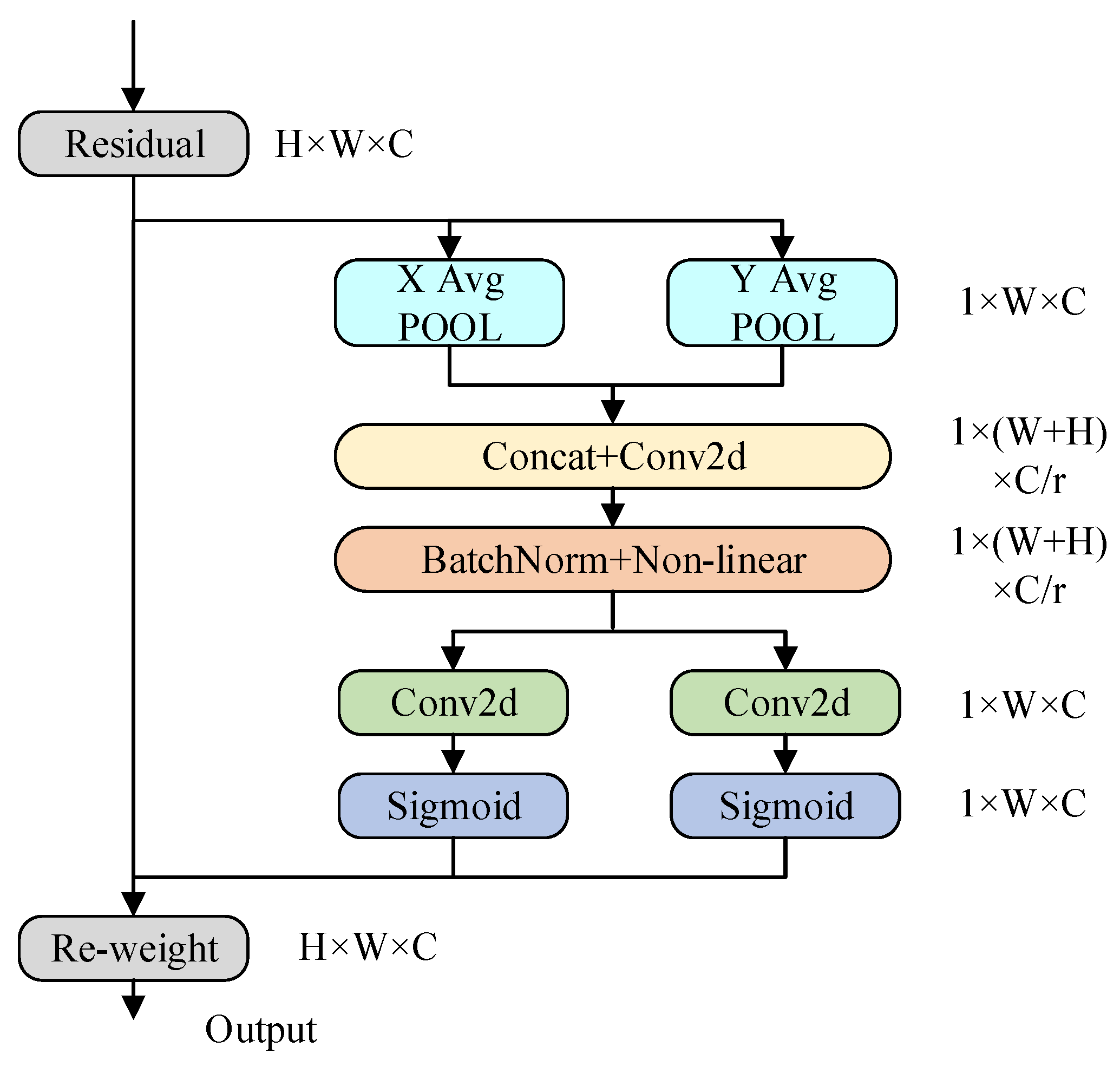
The implementation process of the CA mechanism is shown in Figure 6:

When the CA works, it first performs precise encoding on feature maps of different resolutions. This step aims to complete global pooling along the height and width of the image, resulting in feature maps pooled along the height and width dimensions, respectively.

$$Z_c^h(h)={\displaystyle \frac{1}{W}}{\displaystyle \sum _{0\le i<w}\left|x_c\left(h,i\right)\right.}$$

(2)

$$Z_c^w(w)={\displaystyle \frac{1}{H}}{\displaystyle \sum _{0\le i<H}\left|x_y\left(h,w\right)\right.}$$

(3)

where ${\displaystyle \frac{1}{W}}$ and ${\displaystyle \frac{1}{H}}$ represent the pooled normalization coefficients and $x_c\left(h,i\right)$ and $x_y\left(h,w\right)$ represent the feature values in the original feature map with feature dimensions c and y, spatial positions at $\left(h,i\right)$ and $\left(h,w\right)$.

Then, in order to integrate information across the entire spatial domain, the receptive fields of height and width need to be concatenated, followed by a 1 × 1 convolution to reduce the dimensions to the original size. Finally, the feature map, after being processed by the same BN layer used in MVSNet, is passed through a Sigmoid function to obtain the result, as shown in the following equation:

$$f=\delta \left(F_1\left([z^h,z^w]\right)\right)$$

(4)

where $\delta$ represents a non-linear activation function and $F_1$ represents a 1 × 1 convolutional layer. $\left[\right. ,\left.\right]$ represents a cascade of operations along the spatial dimension.

For the regression of the channel quantity in the feature map, it needs to be performed using a 1 × 1 convolutional kernel. Then, the attention weights in the height and width directions of the image, denoted as $g^h$ and $g^w$, are obtained again through an activation function.

$$g^w=\sigma \left(F_w\left(f^w\right)\right)$$

(5)

$$g^h=\sigma \left(F_h\left(f^h\right)\right)$$

(6)

where $\sigma$ denotes the Sigmoid function.

Finally, in the cost volume, the feature maps carried by each branch are multiplied and weighted, which results in feature maps that carry attention weights in both the height and width dimensions. This is shown in the following equation:

$$y_c\left(i,j\right)=x_c\left(i,j\right)\times g_c^h\left(i\right)\times g_c^w\left(j\right)$$

(7)

3.4. Loss Function

Due to the existence of the “branch” structure in this paper, for branches with larger task scales and more samples, a higher weight is assigned to their loss function, allowing the model to better adapt to the diversity of data. The Loss function in this paper is summed according to the number of branches, as follows ${\displaystyle \sum MVSNe{t}_{loss}}$. The function expression is as follows:

$$Loss={\displaystyle \sum _{p\in P_{valid}}{‖d\left(p\right)-{\widehat{d}}_i\left(p\right)‖}_1+\lambda ·{‖d\left(p\right)-{\widehat{d}}_j\left(p\right)‖}_1}$$

(8)

In Equation (8), $P_{valid}$ is the set of valid pixels in the array, $d\left(p\right)$ is the true depth value of pixel $p$, ${\widehat{d}}_i\left(p\right)$ is the initial depth value of pixel $p$, ${\widehat{d}}_j\left(p\right)$ is the optimized depth value of pixel $p$ and $\lambda$ is the weight coefficient. After applying the Loss function to each resolution, the final Loss function for BCA-MVSNet is obtained by summing the individual Loss functions, as shown in the following equation:

$$Los{s}_{BCA-MVSNet}={\displaystyle \sum _{k=1}^N{\lambda }^k·L^k}$$

(9)

In Equation (9), ${\lambda }^k$ is the weight coefficient, which is set to different values based on the resolution of the “branch.” The higher the resolution, the larger the weight should be set.

4. Experimental Setup

4.1. Experimental Dataset

To demonstrate the generalizability of the BCA-MVSNet model, the DTU dataset [39] and the Tanks and Temples dataset [40] were used for evaluation. In the former dataset, all 2D images were captured indoors on objects like castles and books, and the dataset also provides camera parameters for specific viewpoints of the shooting scenes.

The Tanks and Temples dataset is similar to the scene types that need to be reconstructed in this paper. Both datasets consist of large-scale outdoor scenes. The key difference is that most of the subjects in the Tanks and Temples dataset are outdoor structured objects, such as trains, statues and eight other scene types. In contrast, the scenes to be reconstructed in this paper consist of outdoor scenes without structured objects.

Table 1. DTU and Tanks and Temples dataset information.

Dataset	Training Set	Validation Set	Test Set	Total
DTU	27,097	7546	7546	42,189
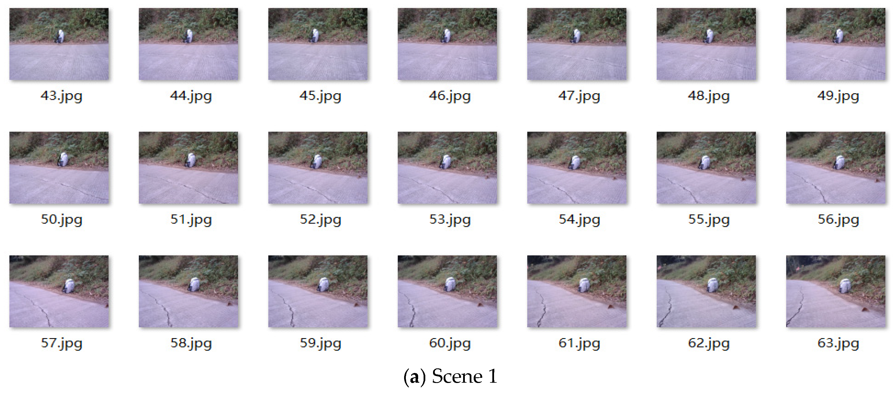
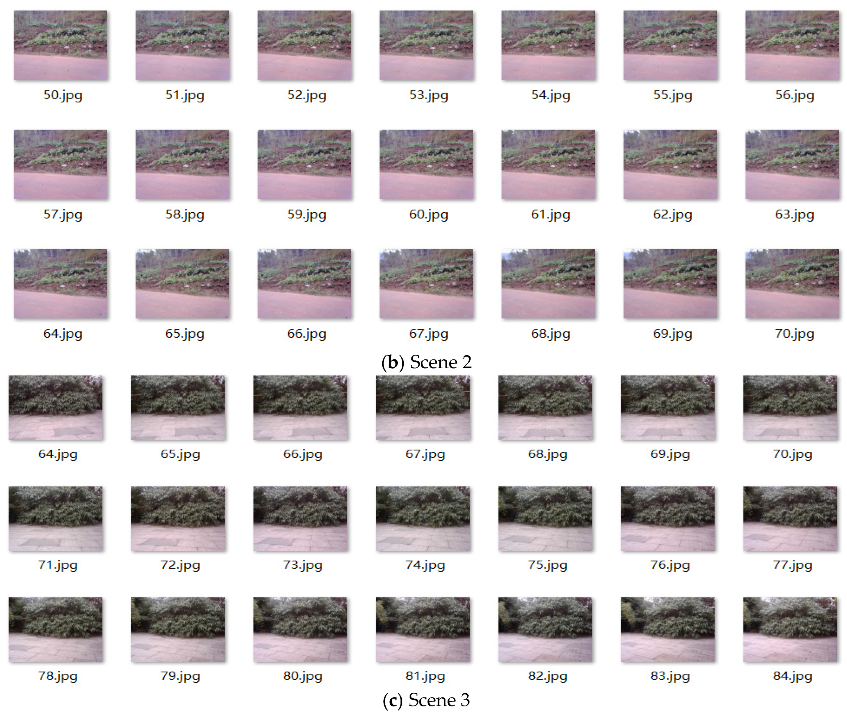
Tanks and Temples	10,000	---	2000	12,000

shows the division of training, testing and validation sets for both the DTU and Tanks and Temples datasets, while Figure 7 presents images of the scenes to be reconstructed in this paper.

In Scenes 1, 2 and 3, this paper used the constructed stereo camera platform to perform circular shooting of the scenes. For Scene 1, the stereo camera captured a total of 71 pairs of 2D images. After left–right separation, 142 2D images with high overlap from different viewpoints were obtained. Scene 2 captured 87 pairs of images, resulting in 174 2D images after separation. Scene 3 captured 105 pairs of images, yielding 210 2D images after left–right separation. Due to the diversity of internal information in the scenes to be reconstructed in this paper, there is a significant increase in the number of circular shots for each individual scene compared to the DTU dataset and others. Additionally, because of the stereo camera, the presence of left–right separation during circular shooting allows for a “twice the effect with half the effort” result.

4.2. Experimental Environment

The experiments in this paper were conducted on a laboratory server. The hardware configuration of the server includes Windows 10 and an NVIDIA TITAN XP 12 GB GPU (Nvidia Corporation, Santa Clara, CA, USA). The software platform used was PyCharm 2023.2.3, with the software environment being Python 3.6.4 and PyTorch 1.12.1. The training of the BCA-MVSNet model on the server took a duration of 21 h.

4.3. Evaluation Index

When using the dataset to assess whether the final reconstruction quality is good, three main evaluation metrics are used: Accuracy (Acc), Completeness (Comp) and Overall Quality. Among them, Overall Quality is determined based on Accuracy and Completeness.

(1) Accuracy (Acc)

The formula for accuracy is as follows:

$$\mathrm{Acc}={\displaystyle \frac{1}{\left|S_1\right|}}{\displaystyle \sum _{x\in S_1,y\in S_2}\min {‖x-y‖}^2}$$

(10)

In Equation (10), $S_1$ represents the reconstructed point cloud, and $S_2$ represents the ground truth point cloud from the dataset. The main task is to evaluate the error between the ground truth point cloud provided by the dataset and the reconstructed point cloud. The accuracy is represented by the average of the shortest distances from any point in the reconstructed point cloud to any point in the ground truth point cloud.

(2) Completeness (Comp)

The implementation of completeness is the exact opposite of accuracy. It starts with the ground truth point cloud provided by the dataset and then calculates the average distance to the reconstructed point cloud. This is expressed as follows:

$$\mathrm{Comp}={\displaystyle \frac{1}{\left|S_1\right|}}{\displaystyle \sum _{x\in S_1,y\in S_2}\min {‖y-x‖}^2}$$

(11)

(3) Overall Quality (Overall)

The value of overall quality is obtained by adding accuracy and completeness and then taking the average. This is expressed as follows:

$$\mathrm{Overall}={\displaystyle \frac{\mathrm{Acc}+\mathrm{Comp}}{2}}$$

(12)

For these three evaluation metrics in 3D reconstruction, a smaller value indicates better reconstruction quality.

4.4. Parameter Setting

In this paper, when BCA-MVSNet is used to train the model, MVSNet and other network settings continue to be used for the selection of values related to parameters. In the deep sampling stage, a uniform sampling strategy with dimensions of [64, 24, 4] is adopted, where the second stage contains 8 sampling values and the third stage contains 4 sampling values. The overall depth sampling number is fixed as 192, the batch size is 4, the optimizer selects Adam, the weight attenuation coefficient is set as 0.00017 and the β parameter is set as (0.9, 0.999). A total of 16 stages were trained, the initial learning rate was adjusted to 0.001 and the learning rate was reduced by 2 times after the 10th, 12th and 14th stages of training.

5. Experimental Analysis

5.1. Experiment and Analysis of DTU Dataset

To demonstrate the excellent performance of the BCA-MVSNet algorithm on the DTU dataset, the qualitative experimental comparison algorithms set are as follows: MVSNet, P-MVSNet, CasMVSNet, TransMVSNet.

5.2. Experimental Analysis of BIFPN Joint Detail-Detection Layer Module

In the BCA-MVSNet network, this paper replaces the feature extraction module with the BIFPN module and adds a detail-detection layer. To validate the effectiveness of this module, BCA-MVSNet is quantitatively analyzed with MVSNet and Cas-MVSNet on the DTU dataset. The results are shown in

Table 2. Quantitative testing of some different algorithms.

Model	Acc/mm	Comp/mm	Overall/mm	Time/s	GPU
MVSNet	0.397	0.517	0.457	2.367	19.6
Cas-MVSNet	0.345	0.429	0.387	1.727	8.36
BCA-MVSNet	0.313	0.417	0.365	1.836	10.07

.

In Table 2, the bold font indicates the best-performing network structure, and the underlined text indicates the second-best network structure. Compared to MVSNet and Cas-MVSNet, BCA-MVSNet (CA removed) using only BIFPN performed better in terms of accuracy, completeness and overall quality. It reduces Acc by 0.052 mm and 0.084 mm, reduces Comp by 0.088 mm and 0.1 mm and reduces Overall by 0.088 mm and 0.092 mm, respectively. MVSNet, due to the presence of an 8-layer unidirectional convolutional neural network, is not able to effectively extract and learn feature information. In comparison to Cas-MVSNet, BCA-MVSNet bridges the information exchange between different resolutions. The depth map results and point cloud effect comparisons of the above algorithms on the DTU dataset for some images are shown in Figure 8 and Figure 9.

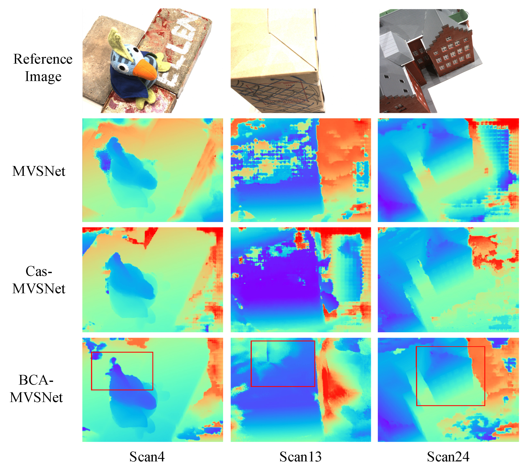
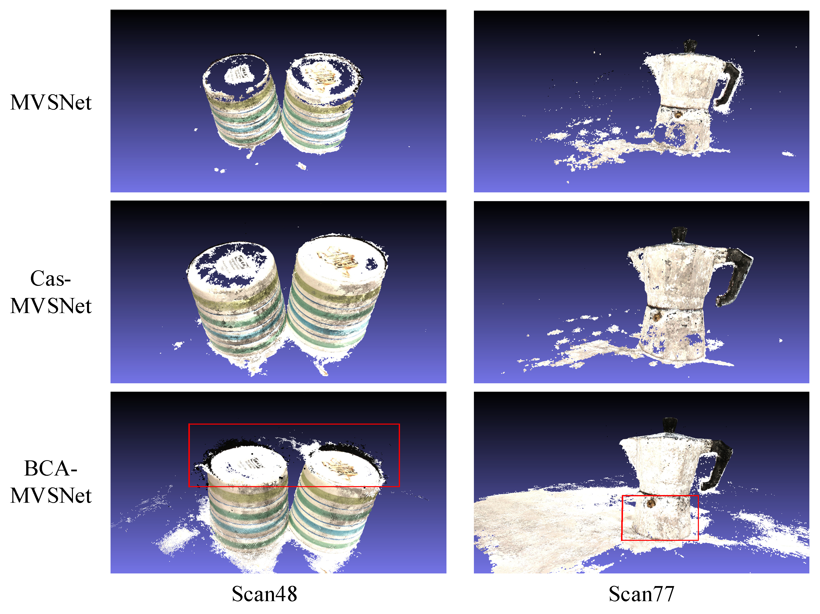
In Figure 8, the depth map comparison for three different network algorithms on the DTU dataset clearly shows that the depth maps of the three scenes in the BCA-MVSNet algorithm present smoother and clearer textures in the key information areas (red-box areas). In Scan4, the “comb” area of BCA-MVSNet is noticeably more complete and cohesive, while the other two network structures exhibit some missing parts. In Scan24, for the “building” windows, the other two network structures no longer show distinct window frames. From the point cloud effect comparison, the red-box area is where BCA-MVSNet outperforms the other two network structures, which indicates that BCA-MVSNet is better at capturing information from flat and weak-texture regions, resulting in more complete 3D point cloud effects.

In summary, it can be concluded that the feature extraction part of the BCA-MVSNet network, due to the presence of BIFPN and the detail-detection layer, allows the BCA-MVSNet network to achieve better depth map and point cloud effects compared to other algorithms. This confirms the effectiveness of the improvements made in the feature extraction part.

BIFPN adopts a multi-scale feature fusion strategy, which enables the network to learn features at different resolution levels. Through bidirectional fusion, that is, backward propagation from high resolution to low resolution and from low resolution to high resolution, it fully excavates the detailed information at all levels. This two-way feature fusion ensures that the network can not only capture the global macroscopic features, but also process the local details in a refined way, so as to restore the depth information and geometric structure more accurately in the reconstruction process. Through its bidirectional feature fusion and detail enhancement capabilities, the network can extract and utilize features of different scales more accurately, and significantly improve the quality of depth maps and point clouds. This improvement ensures that BCA-MVSNet can better handle details and global information in complex scenes, thus effectively improving the accuracy and robustness of 3D reconstruction.

5.3. Experimental Analysis of CA Module in the Cost Body

The preceding stage of the probability volume, the cost volume’s ability to learn spatial and feature information is extremely important. In this paper, only the CA module from BCA-MVSNet is used, and a quantitative comparison is made with the MVSNet and Cas-MVSNet algorithms, as shown in

Table 3. Quantitative comparison between different algorithms.

Model	Acc/mm	Comp/mm	Overall/mm	Time/s	GPU
MVSNet	0.397	0.517	0.457	2.367	19.3
Cas-MVSNet	0.345	0.429	0.387	1.727	9.61
BCA-MVSNet	0.324	0.428	0.376	1.948	11.37

.

In Table 3, the bold font indicates the best-performing network structure, and the underlined text indicates the second-best network structure. It can also be seen that, with only the addition of the CA module, the BCA-MVSNet network still outperforms the other two network algorithms. The Acc is reduced by 0.073 mm and 0.021 mm, respectively; the Comp is reduced by 0.089 mm and 0.001 mm, respectively and the Overall is reduced by 0.07 mm and 0.011 mm, respectively. In terms of time, due to the presence of the CA module, BCA-MVSNet takes slightly longer than the Cas-MVSNet network. However, sacrificing a minimal amount of time to ensure higher accuracy is worthwhile. Similarly, comparisons of depth maps and point cloud effects are shown in Figure 10 and Figure 11.

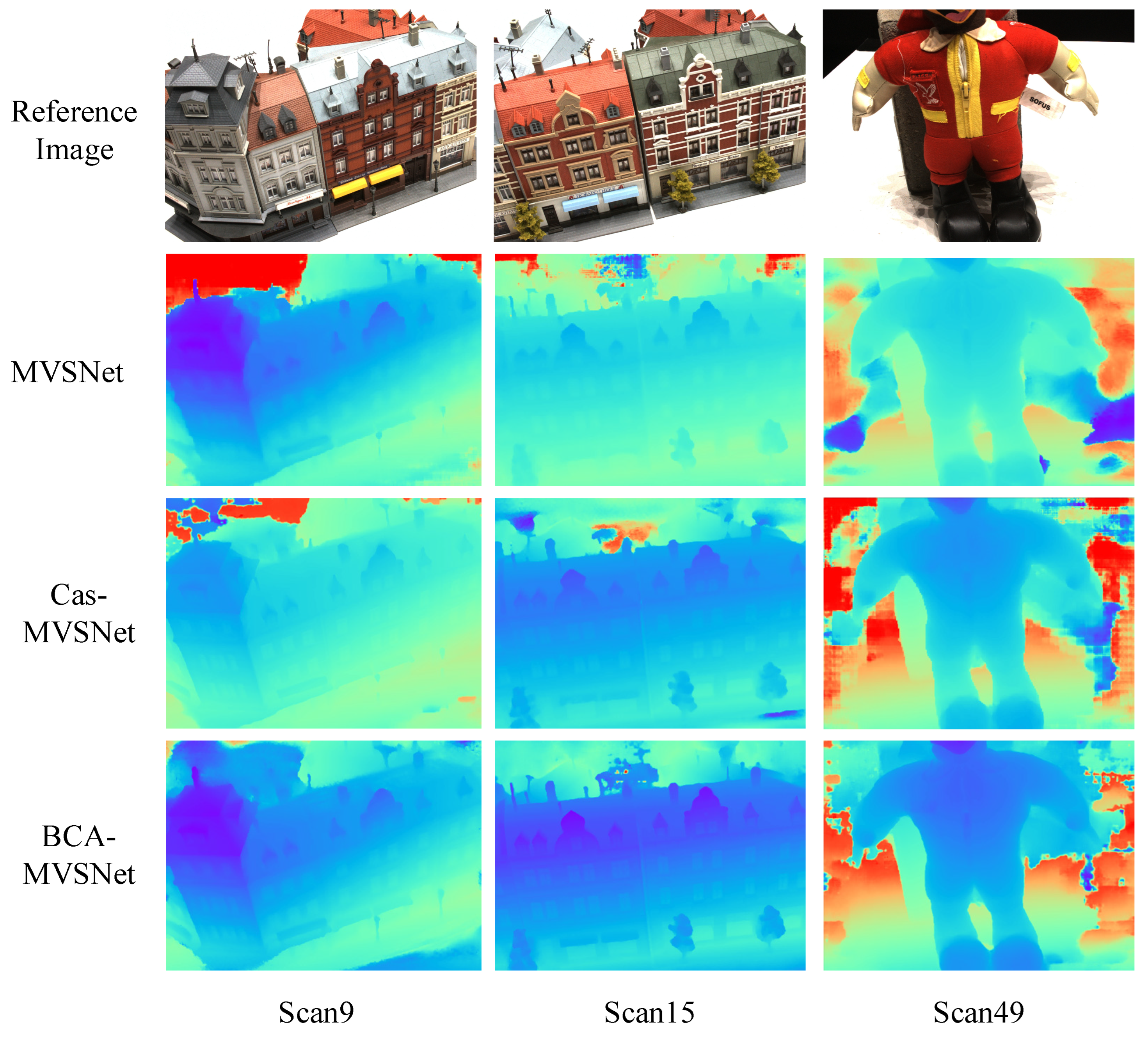
In the above Figure 10, there is no need to highlight the difference in depth maps between the BCA-MVSNet network and the other networks with a red box. It can be clearly seen that, relying on the CA module, the BCA-MVSNet network is more sensitive to spatial information. This is reflected in the depth map of BCA-MVSNet, which shows clearer texture details and better separation of foreground and background layers, without large areas of noise or mixed information from different depths. At the same time, the point cloud comparison between BCA-MVSNet and other algorithms is shown in Figure 11.

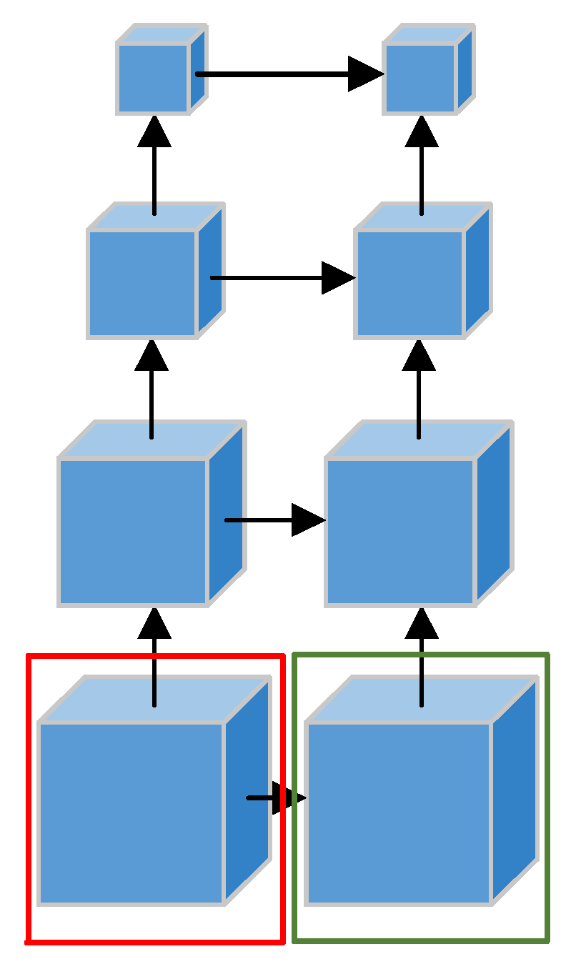
From the red box in the Scan15 comparison image, it can be seen that the visualized point cloud is more complete regarding subtle details. Moreover, the point cloud holes caused by occlusion are fewer in the BCA-MVSNet network. After incorporating the CA module, the BCA-MVSNet network is able to enhance point cloud integrity. In the green box comparison in Scan49, the MVSNet network directly misses the point cloud information of the “head,” while the Cas-MVSNet network has poorer reconstruction results for the “hand” and “badge.” The BCA-MVSNet network shows good point cloud texture in all three of these areas. In summary, the introduction of the CA module in the cost body section of BCA-MVSNet enhances the learning ability for feature bodies. This ensures that the information extraction improvements made in the feature extraction stage are not wasted.

The CA module effectively integrates feature information from different perspectives through a fine feature aggregation strategy, which enriches feature expression and improves accuracy. It not only enhances the expression of local features, but also integrates global context information to help the model better understand complex geometric structures, especially when dealing with occluded areas and complex scenes, reducing the error in depth estimation. By optimizing the detail information in the feature extraction stage, the CA module ensures that these details are effectively retained in the cost body link, and avoids information loss through multi-scale and inter-level information transmission, so as to accurately map to the final 3D model and improve the reconstruction accuracy.

5.4. Overall Comparison Experiment

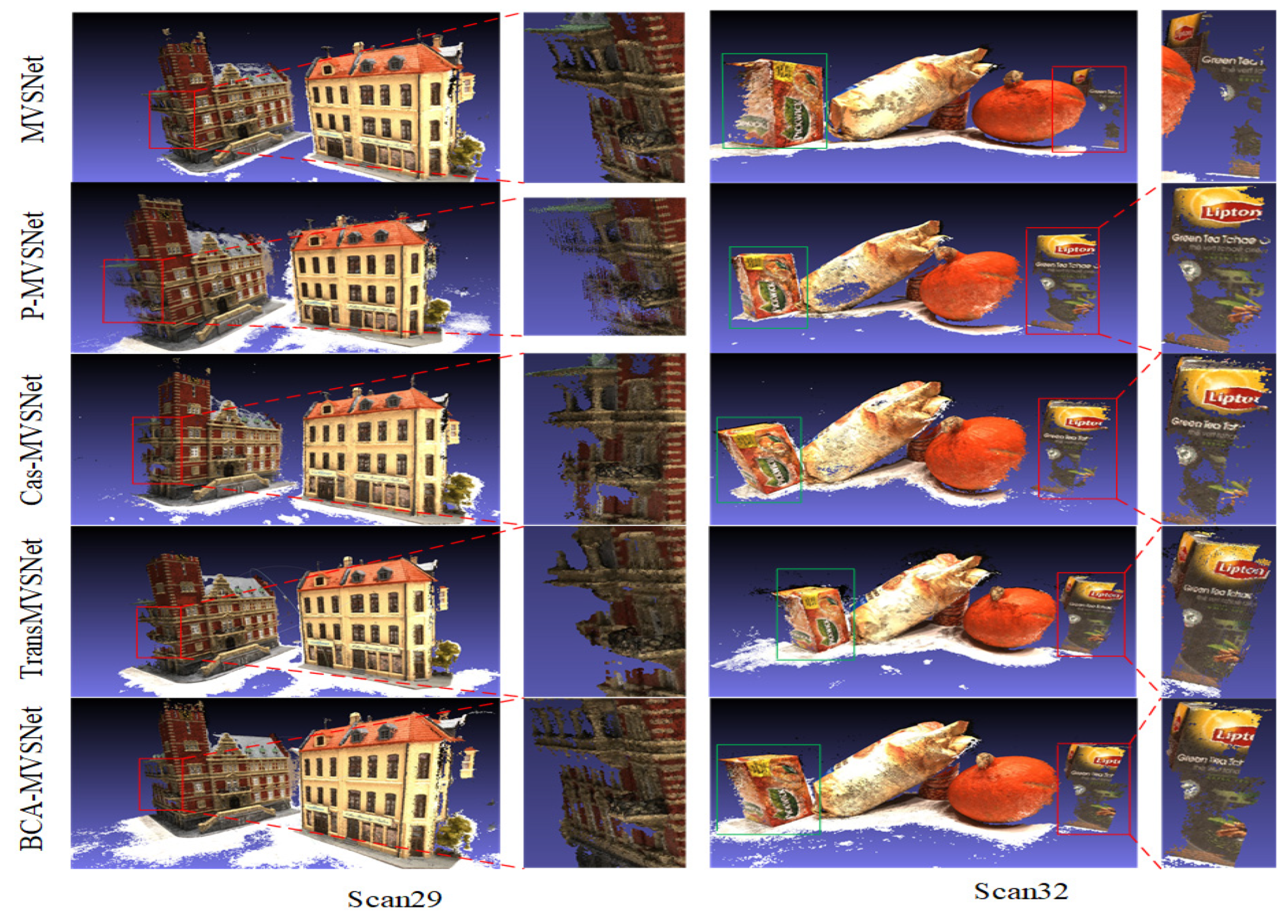
Comparing the BCA-MVSNet network presented in this paper with the basic MVSNet network, the P-MVSNet network equipped with anisotropic convolution, the Cas-MVSNet network which derives depth maps based on different resolutions and the TransMVSNet network that incorporates the Transformer module, the point cloud comparison images are shown in Figure 12 and Figure 13.

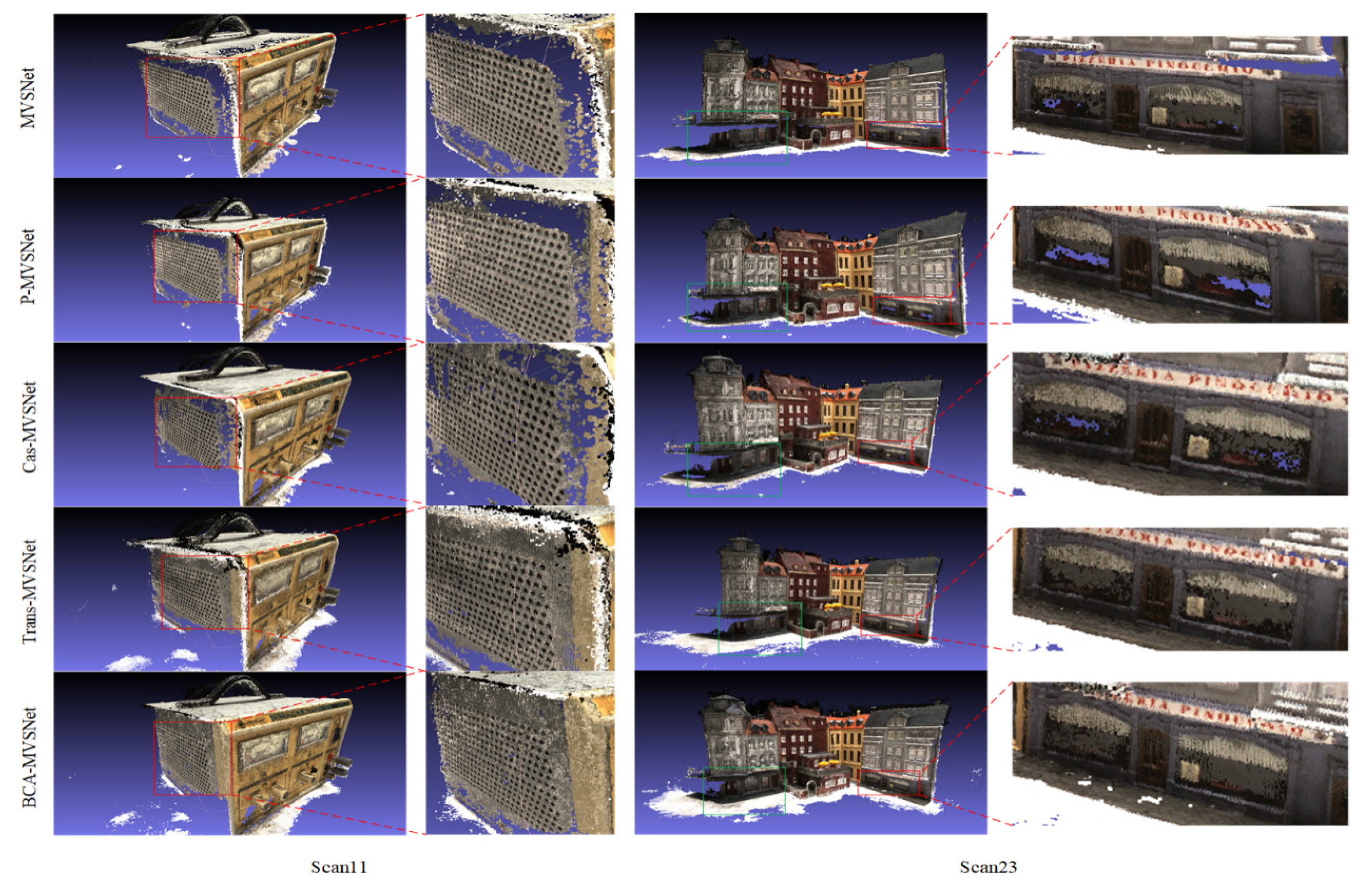
From Scan11 in Figure 12 and Scan29 in Figure 13, it can be seen that among the five different network structures, BCA-MVSNet achieved the best reconstruction results for certain areas without multiple views of some textures during multi-view circular shooting, especially the point cloud information on the side of the 3D model, which is the most comprehensive. In Scan11, MVSNet, P-MVSNet and Cas-MVSNet all show large continuous holes in the red-boxed area, while TransMVSNet, second only to the BCA-MVSNet network in this paper, produces no large holes. In Scan29, the red-boxed area “castle” has the richest detail information in BCA-MVSNet, while other network structures show varying degrees of distortion and holes.

In Scan23 and Scan32, no magnification was applied to the green-boxed areas since the contrast was sufficiently clear. In the green-boxed area of Scan23, it is clear that the BCA-MVSNet network has almost no holes compared to the other four network structures. In the green-boxed area of Scan32, BCA-MVSNet shows some slight distortion at the boundaries compared to P-MVSNet but still performs significantly better than the other three networks. In the red-boxed area comparisons in Scan23 and Scan32, BCA-MVSNet’s excellent performance in point cloud completeness is evident.

To further highlight and compare the differences and advantages of the different network structures, this paper introduces two additional comparison algorithms: R-MVSNet, H-MVSNet and Fast-MVSNet. The descriptions of these three network structures are as follows:

(1)

R-MVSNet: Developed by the same authors as MVSNet, this network structure adds a recurrent neural network (RNN) to the MVSNet framework to reduce GPU consumption.

(2)

H-MVSNet: The network structure is set from coarse to fine to optimize depth map generation.

(3)

Fast-MVSNet: Introduces Gaussian–Newton refinement in the depth feature domain for extraction, while also offering high real-time performance.

The quantitative results are shown in

Table 4. Quantitative testing of DTU datasets.

Model	Acc/mm	Comp/mm	Overall/mm	Time/s	GPU
MVSNet	0.396	0.524	0.460	3.71	22.5
R-MVSNet	0.381	0.476	0.429	6.17	6.9
P-MVSNet	0.386	0.493	0.440	3.24	10.4
H-MVSNet	0.408	0.393	0.401	4.63	9.46
Cas-MVSNet	0.371	0.426	0.399	2.12	9.9
TransMVSNet	0.286	0.678	0.482	3.04	13.08
Fast-MVSNet	0.342	0.364	0.353	1.74	8.79
BCA-MVSNet	0.361	0.327	0.344	2.62	11.6

.

As shown in Table 4, the bold font indicates the best-performing network structure, and the underlined text indicates the second-best network structure. In terms of accuracy, TransMVSNet performs the best among the eight network structures, while Fast-MVSNet ranks second due to its feature refinement operations. However, TransMVSNet does not perform well in terms of completeness, overall quality and time consumption, it ranks second to last in GPU consumption, it is difficult to adapt to large-scale reconstruction and in the weak-texture area, its attention allocation is vulnerable to noise interference. In contrast, the BCA-MVSNet network in this paper performs excellently in both completeness and overall quality, especially with completeness leading the second-place Fast-MVSNet network by 0.037. In terms of time and GPU consumption, although this paper has utilized depth map calculation at different resolutions separately based on the Cas-MVSNet network, the introduction of BIFPN, the detail-detection layer and the CA module means that it does not achieve the best performance among these eight algorithms. However, for weak-texture regions, the combination of BIFPN and CA module shows significant advantages. BIFPN can better deal with multi-scale features through the structure of two-way feature pyramid network, while the CA module enhances the correlation of global and local context information through fine feature aggregation strategy. This combination of BIFPN and CA can effectively compensate for the lack of feature information in weak-texture regions and improve the accuracy of depth estimation. Especially in terms of detail richness and depth accuracy, the combination of BIFPN and CA has significantly improved the performance of the model in complex environments.

In conclusion, the BCA-MVSNet network sacrifices some real-time performance and GPU consumption while ensuring the quality of point cloud reconstruction, which is beneficial for the reconstruction tasks of the scene types considered in this paper.

5.5. Experiment and Analysis of the Tanks and Temples Dataset

The Tanks and Temples dataset has similar scene characteristics to the reconstruction tasks in this paper, both featuring large-scale structures and covering large areas with weak-texture regions. To test the generalization ability of the BCA-MVSNet model, it was trained on the DTU dataset and then directly applied to the Tanks and Temples dataset for testing. In terms of parameter settings, the same parameters as before were used, but the depth sample number was set to 96. The quantitative test results of different networks on the Tanks and Temples dataset are shown in

Table 5. Quantitative testing on the Tanks and Temples dataset (higher is better).

Model	Mean	Family	Francis	Horse	Lighthouse	M60	Panther	Playground	Train
MVSNet	42.99	56.13	29.47	24.16	49.76	51.09	48.34	48.3	36.7
R-MVSNet	46.12	65.97	34.49	33.19	43.19	49.88	46.6	53.73	41.91
P-MVSNet	49.39	61.73	42.26	36.13	52.1	52.63	51.77	53.46	45.09
H-MVSNet	49.74	61.95	44.64	36.76	51.83	53.17	50.73	52.9	45.93
Cas-MVSNet	46.17	59.93	32.6	32.37	52.63	51.11	49.45	52.6	38.74
TransMVSNet	49.52	62.16	39.50	40.57	50.40	55.32	52.12	51.83	44.27
Fast-MVSNet	49.37	62.4	32.47	30.26	63.73	53.29	54.17	55.94	42.73
BCA-MVSNet	52.75	68.18	53.26	41.74	54.6	51.83	47.95	58.1	46.38

. The partial reconstruction results of the BCA-MVSNet network on the Tanks and Temples dataset are displayed in Figure 14. the bold font indicates the best-performing network structure.

As shown in Table 5, the BCA-MVSNet model demonstrates strong generalization ability. For the outdoor scenes in the Tanks and Temples dataset, the unmodified Cas-MVSNet model performs poorly overall, only outperformed by the MVSNet network. However, for certain scenes in the Tanks and Temples dataset, both TransMVSNet and Fast-MVSNet networks perform well, thanks to their strong ability to extract and learn weak-texture details. Overall, the BCA-MVSNet network performs well on large-scale weak-texture scenes in the dataset, capable of generating complete point cloud models with no loss of texture information.

5.6. Experiment and Analysis of Self-Made Dataset

In Figure 15a–c, the results of capturing three scenes to be reconstructed using a stereo camera are shown. In this section, the segmented partial images of these three scenes are displayed in Figure 15.

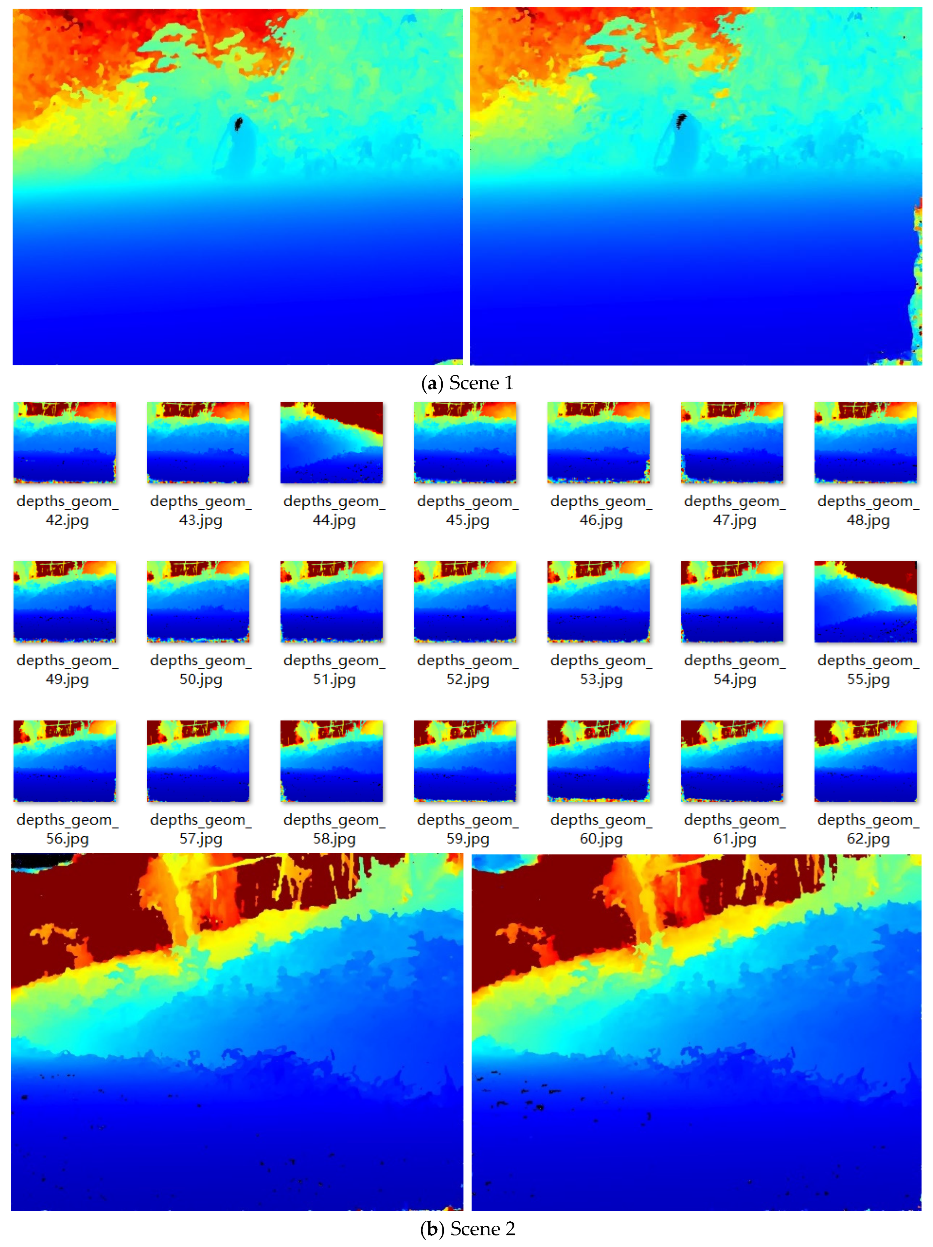
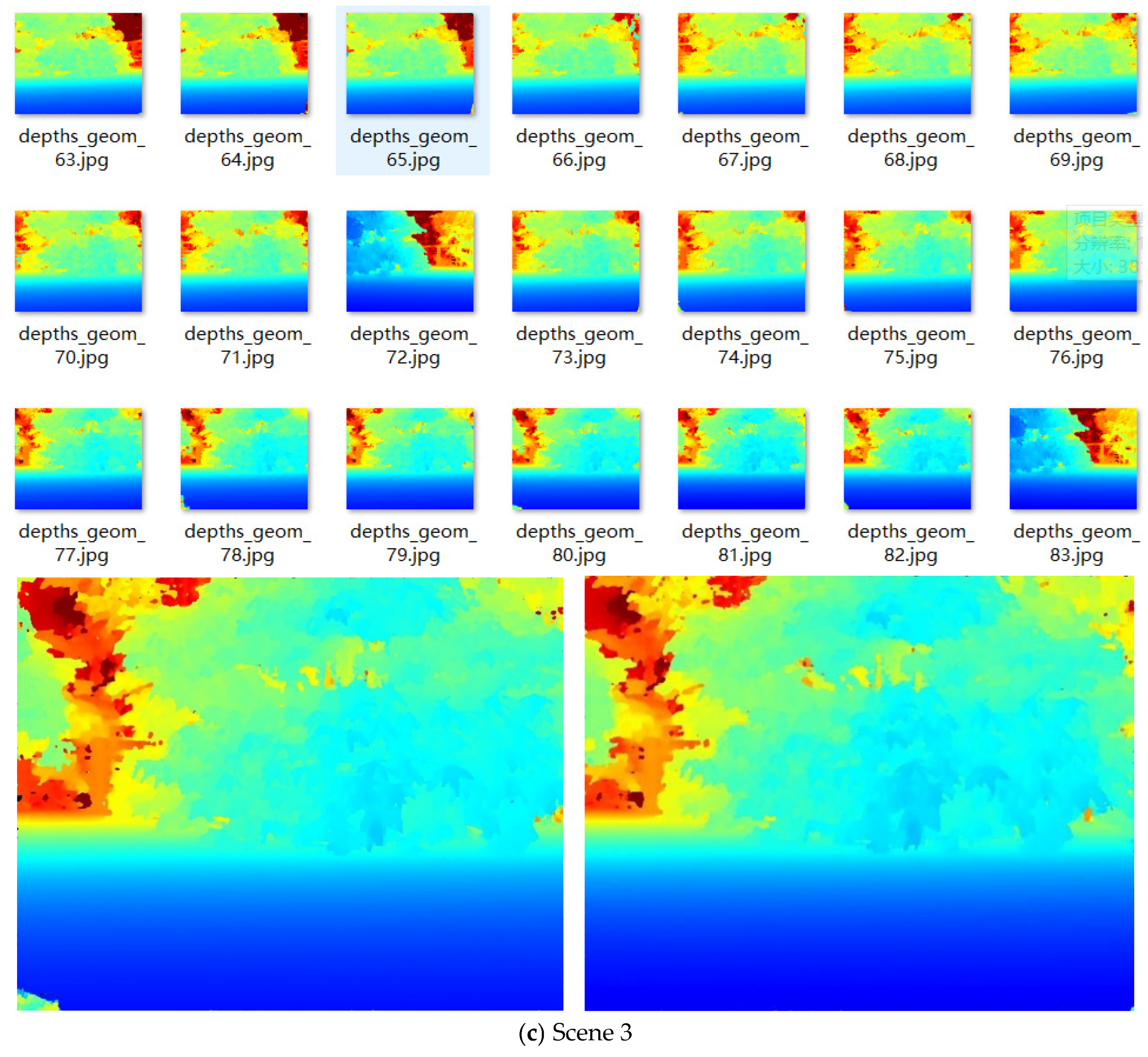
By using the camera parameters for each shot provided in this paper, combined with the BCA-MVSNet network model, the partial depth maps of the three scenes are shown in Figure 16.

In Figure 16, it can be observed that the BCA-MVSNet algorithm, due to its focus on the limited detail information in weak-texture areas and the CA module in the cost volume that enhances feature learning, produces depth maps with good depth-texture information for all three scenes. In particular, the weak-texture areas in the three scenes are notably smooth with no large voids. After post-processing the depth maps, the final point cloud result is shown in Figure 17.

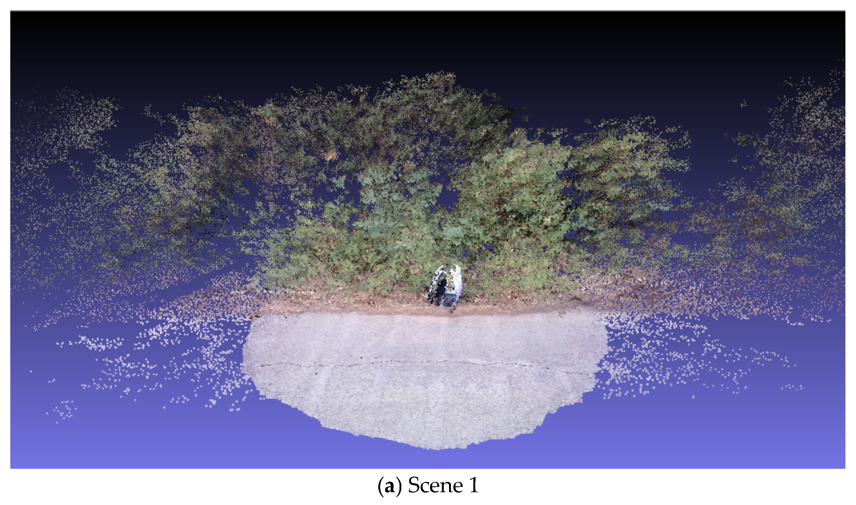
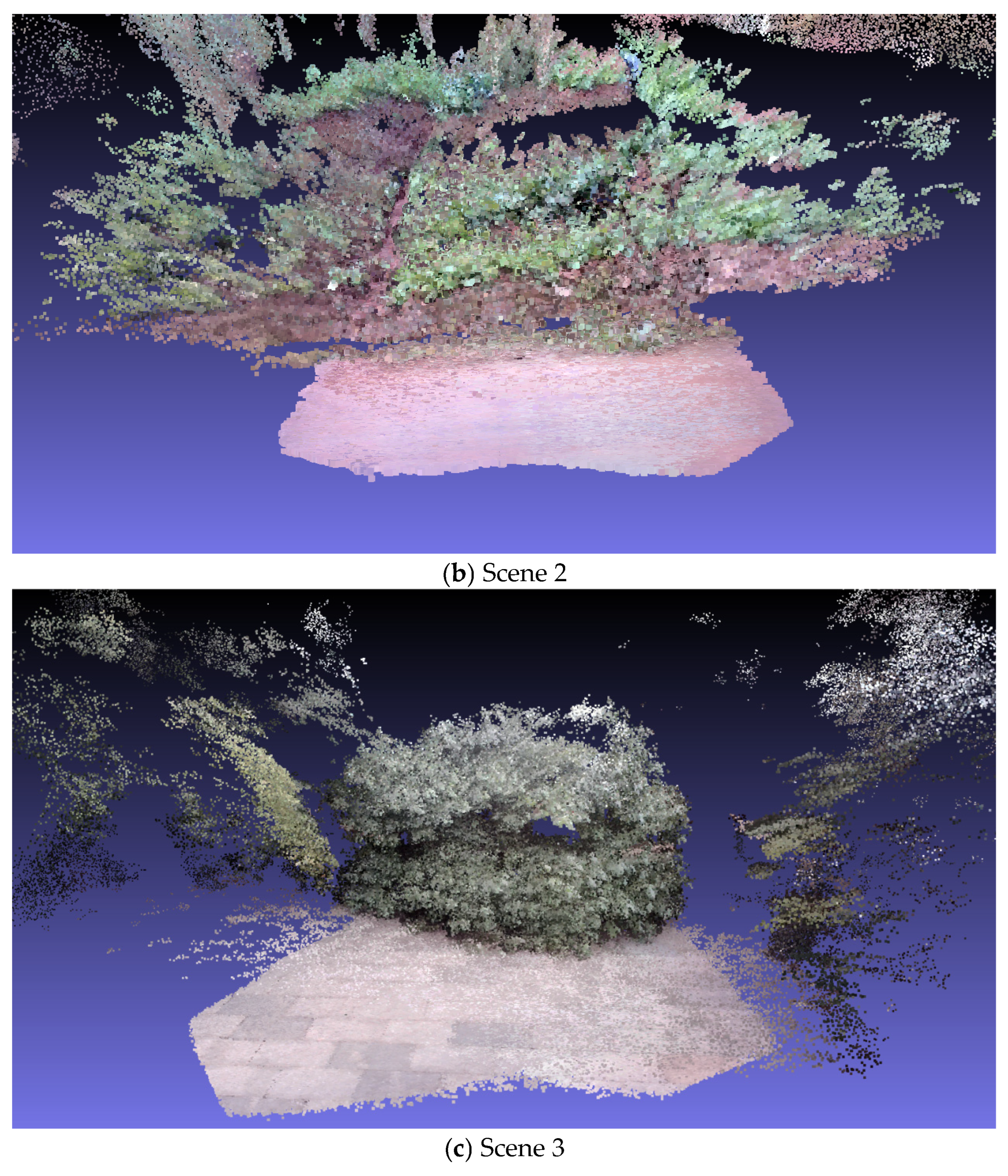
To further restore the authenticity of the scenes and better adapt to engineering projects, this paper performed texture mapping on the point cloud results of the three scenes. The final 3D models are shown in Figure 18.

It can be seen that the three scenes are unstructured, large-scale outdoor scenes with weak textures. After being captured by the stereo camera in a surrounding manner, and by combining the camera parameters and images through the BCA-MVSNet network, the final 3D models are able to capture all the nearby information. After texture mapping, no voids are generated in the weak-texture areas, and details such as cracks in the road and boundaries between tiles are clearly visible. The accuracy has reached a level suitable for engineering projects.

The robustness of weak-texture regions and the ability of cross-scale feature fusion demonstrated in multi-view depth estimation in this study allow it to have application potential in many fields: in the field of medical imaging, it can reduce the artifacts caused by respiratory motion through the cross-view consistency verification of BIFPN for the 3D reconstruction needs of organ soft-tissue (weak-texture features) and the spatial attention mechanism of the CA module can focus on the edge of the lesion (such as the boundary between tumor and normal tissue); in the navigation of an indoor robot, facing the weak-texture environment of furniture surfaces (such as a smooth desktop), white walls and the like, the method can generate a dense depth map by rapidly aggregating multi-frame visual information, provide reliable geometric constraint for obstacle avoidance and path planning and adapt to an embedded computing platform of the robot; in the task of digitizing historical sites, for scenes such as weathered stone (surface texture is blurred) and large sculptures (multi-scale features coexist), the two-way feature transfer of BIFPN can preserve detailed textures (such as sculpture lines), while the CA module can enhance the consistency of features under different shooting angles and reduce the reconstruction deviation caused by illumination changes (such as direct sunlight and shadow areas).

However, the study also found two major limitations: on one hand, in large-scale scene reconstruction, the cross-view fusion efficiency of BiFPN decreases linearly with the increase in the number of views; on the other hand, for the reconstruction of completely texture-free regions, it still relies mainly on geometric constraints, and the feature matching accuracy is lower than that of texture-rich regions. In order to solve these problems, future research can make breakthroughs in two directions: one is to enhance the constraints of texture-free regions by combining semantic prior information; the other is to explore a lightweight fusion mechanism based on graph neural networks to improve the computational efficiency in large-scale scenes.

6. Conclusions

This paper uses a stereo camera for the MVS reconstruction task based on deep learning. To make the network structure meet the requirements of unstructured, weak-texture, large-scale scenes, the following improvements were made to the Cas-MVSNet network. First, the feature extraction network was replaced with the BIFPN to enhance the integration between low-level and high-level information. Next, a detail- and fine-texture-detection layer was added to the BIFPN structure. The purpose of this layer is to avoid missing the already scarce texture information in weak-texture areas, ensuring that the feature information of this part is retained during feature extraction. Finally, the CA module was introduced in the cost volume stage, making the learning of the feature volume more focused and ensuring high attention both spatially and channel-wise.

In the end, the BCA-MVSNet network was compared qualitatively and quantitatively with other algorithms on the DTU and Tanks and Temples datasets. The comparison results show that, overall, it performs better both in terms of depth maps and point cloud results. Additionally, by using the stereo camera built in this paper to capture the reconstruction scene in a surrounding manner, and combining the camera parameters, the 3D models obtained through the BCA-MVSNet network achieved texture authenticity in weak-texture areas that meets the accuracy required for engineering projects.