A Quantitative Analysis Framework for Investigating the Impact of Variable Interactions on the Dynamic Characteristics of Complex Nonlinear Systems

Abstract

The proliferation of power electronics in renewable-integrated grids exacerbates the challenges of nonlinearity and multivariable coupling. While the modal series method (MSM) offers theoretical foundations, it fails to provide tools to systematically quantify dynamic interactions in these complex systems. This study proposes a unified nonlinear modal analysis framework integrating second-order analytical solutions with novel nonlinear indices. Validated across diverse systems (DC microgrids and grid-connected PV), the framework yields significant findings: (1) second-order solutions outperform linearization in capturing critical oscillation/damping distortions under realistic disturbances, essential for fault analysis; (2) nonlinear effects induce modal dominance inversion and generate governing composite modes; (3) key interaction mechanisms are quantified, revealing distinct voltage regulation pathways in DC microgrids and multi-path dynamics driving DC voltage fluctuations. This approach provides a systematic foundation for dynamic characteristic assessment and directly informs control design for power electronics-dominated grids.

1. Introduction

With the rapid development of renewable energy, such as wind and solar power, the proportion of power electronic devices in the power grid has increased significantly, which has paved the way for new power grids with high flexibility, sustainability, and improved efficiency. Yet, it also poses new challenges to the stability of the power system [1,2]. Compared to traditional power systems dominated by synchronous generators, the new-type power system exhibits considerable nonlinearity, time variability, and uncertainty [3]. These characteristics force the dynamic process of the power grid to emerge more complex properties when suffering from disturbances. Furthermore, the new-type power grid consists of numerous power electronic devices assembled with a multiple-time scale control system for regulating the current and voltage for the integration system, which results in the interaction of the controllers and thus may cause various stability problems during transient conditions.

Power system dynamic analysis is intrinsically governed by the mechanisms underlying convergence behavior and equilibrium stability. Small-signal linearization techniques, utilizing eigenvalue analysis and frequency domain methods [4], have been widely applied to investigate oscillation mechanisms [5], harmonic patterns [6,7], and control parameter design [8]. However, this perspective introduces inherent limitations as the truncation of higher-order terms in Taylor expansions restricts its validity to systems with limited nonlinear components.

Consequently, nonlinear analysis methods are essential for capturing large-signal stability phenomena, focusing on trajectory convergence, attraction domain boundaries, and post-disturbance evolution. These methods mainly consist of Lyapunov functions [9,10,11,12] and the higher-order modal analysis method [13,14,15,16,17]. Lyapunov-based methods, despite their mathematical rigor, face inherent limitations in high-dimensional power systems due to theoretical conservatism and the absence of universal Lyapunov function construction rules, which hinders their practical implementation.

In contrast, the higher-order modal analysis method provides an intuitive alternative by decomposing system dynamics into modes, enabling direct visualization of state evolution and dominant oscillatory behaviors. The normal form method (NFM) [13,14] and the modal series method (MSM) [15,16,17] are two commonly used approaches. However, the NFM has limitations: the variables obtained after its nonlinear transformation often lose their physical meaning, and it is not suitable for systems with second-order or higher-order resonance conditions [17]. Conversely, the MSM enables the derivation of an approximate closed-form solution for the response of a nonlinear system through linear state-space transformation, thereby showcasing a broader scope of application and higher accuracy, making it a more robust choice for complex system analysis. For example, the literature [18] analyzes the nonlinear interactions between unified power flow controllers and power systems. The coupling mechanisms among various components in renewable energy systems have been discussed in [19,20].

Despite its theoretical foundation and demonstrated capabilities, the practical application of conventional MSM remains underdeveloped for systematically characterizing the complex, multi-variable dynamic interactions prevalent in modern, renewable-rich power grids. Specifically, there is a critical need for an operational framework based on MSM that can effectively quantify and disentangle the coupling mechanisms among numerous state variables during transient events.

This study bridges this critical gap by advancing nonlinear modal analysis into an operational framework to systematically characterize multivariable coupling mechanisms during transient processes. We propose an analytical paradigm that enhances conventional nonlinear dynamic assessment through specifically devised interaction indices. Through case validation, the framework demonstrates precise identification of dominant variables governing disturbance-response dynamics in nonlinear systems and elucidates coupling effects across nonlinear modes.

The paper is organized as follows: Section 2 reviews the MSM and derives the second-order analytical solutions. Building on this theoretical framework, a set of nonlinearity indices is proposed to quantify variable interactions systematically. To validate the proposed framework and indices, Section 3 develops mathematical models and control strategies for two experimental platforms: (1) a three-unit photovoltaic (PV)-storage DC microgrid and (2) a grid-connected PV system. Comprehensive case studies on both platforms confirm the indices’ effectiveness in capturing key dynamics and interactions, demonstrating their broad applicability. Finally, Section 4 provides critical discussions and conclusive remarks.

2. System Modeling and Dynamic Analysis

2.1. Approximate Solutions for System Responses

The dynamics of the power system can be described as follows:

$$\dot{\mathit{X}}=\mathit{f}(\mathit{X})$$

(1)

where X denotes an N-dimensional state variable. Equation (1) can be expanded in a Taylor Series around the equilibrium point of X_sep:

$${\dot{x}}_i=A_{i}X+{\displaystyle \frac{1}{2}}{\displaystyle \sum _{k=1}^N{\displaystyle \sum _{l=1}^N{H}_{kl}^i}}{x}_k{x}_l+o\left(|X{|}^3\right)$$

(2)

where i = 1, 2, …, N; A_i is the ith row of the Jacobian matrix A = (∂f/∂X)|_Xsep; Hⁱ = (∂f_i/∂x_kx_l)|_Xsep is the ith Hessian matrix. It is assumed that X belongs to the convergence domain of the Taylor Series.

Assuming the system has N distinct eigenvalues, U and V represent the normalized right and left eigenvector matrices of A, satisfying V^T = U⁻¹, that is

$$V^{T}U=I$$

(3)

Let X = UY, and the equivalent differential equation is derived as follows:

$${\dot{y}}_j={\lambda }_j{y}_j+{\displaystyle \sum _{k=1}^N{\displaystyle \sum _{l=1}^N{C}_{kl}^j}}{y}_k{y}_l+o\left(|Y{|}^3\right)$$

(4)

$$C^j={\displaystyle \frac{1}{2}}{\displaystyle \sum _{p=1}^N{v}_{jp}}\left[U^{\mathrm{T}}{H}^{p}U\right]$$

(5)

where j, p = 1, 2, …, N; v_jp is the jth row and the pth column of V^T; λ_j is the jth eigenvalue; H^p is the pth Hessian matrix; $C_{kl}^j$ denotes the element of matrix ${\mathit{C}}^j$ located at row i, column j.

Under the condition that λ_k + λ_l ≠ λ_j, applying the MSM in [20] to solve Equation (4) yields the second-order solution for the system’s response:

$$y_j(t)=\left(y_{j0}-{\displaystyle \sum _{k=1}^N{\displaystyle \sum _{l=1}^N{h}_{2,kl}^j}}{y}_{k0}{y}_{l0}\right){\mathrm{e}}^{{\lambda }_{j}t}+{\displaystyle \sum _{k=1}^N{\displaystyle \sum _{l=1}^N{h}_{2,kl}^j}}{y}_{k0}{y}_{l0}{\mathrm{e}}^{\left({\lambda }_k+{\lambda }_l\right)t}$$

(6)

where y_j0 is the jth element of Y₀, Y₀ = U⁻¹X₀ = V^TX₀, representing the initial value vector of the Y, X₀ is the initial value vector of the X.

The nonlinear coefficient $h_{2,kl}^j$in (6) can be calculated as follows:

$$h_{2,kl}^j={\displaystyle \frac{C_{kl}^j}{{\lambda }_k+{\lambda }_l-{\lambda }_j}}$$

(7)

Apply an inverse transformation to (6), we can derive the closed-form second-order solution of the original system:

$$x_{2,i}(t)={\displaystyle \sum _{j=1}^N{u}_{ij}}\left(y_{j0}-{\displaystyle \sum _{k=1}^N{\displaystyle \sum _{l=1}^N{h}_{2,kl}^j}}{y}_{k0}{y}_{l0}\right){\mathrm{e}}^{{\lambda }_{j}t}+{\displaystyle \sum _{j=1}^N{u}_{ij}}{\displaystyle \sum _{k=1}^N{\displaystyle \sum _{l=1}^N{h}_{2,kl}^j}}{y}_{k0}{y}_{l0}{\mathrm{e}}^{\left({\lambda }_k+{\lambda }_l\right)t}$$

(8)

The second-order solution of the ith state value is composed of two distinct complex summation expressions, which are defined separately for clarity:

$$L_{2i}\triangleq {\displaystyle \sum _{j=1}^N{u}_{ij}}\left(y_{j0}-{\displaystyle \sum _{k=1}^N{\displaystyle \sum _{l=1}^N{h}_{2,kl}^j}}{y}_{k0}{y}_{l0}\right){\mathrm{e}}^{{\lambda }_{j}t}$$

(9)

$$N_{2i}\triangleq {\displaystyle \sum _{j=1}^N{u}_{ij}}{\displaystyle \sum _{k=1}^N{\displaystyle \sum _{l=1}^N{h}_{2,kl}^j}}{y}_{k0}{y}_{l0}{\mathrm{e}}^{\left({\lambda }_k+{\lambda }_l\right)t}$$

(10)

where u_ij is the element at the ith row and the jth column of U; y_k0 and y_l0 are the kth and lth elements of Y₀.

Similarly, the first-order closed-form solution can be obtained as follows:

$$x_{1,i}(t)={\displaystyle \sum }_{j=1}^N{u}_{ij}{y}_{j0}{\mathrm{e}}^{{\lambda }_{j}t}$$

(11)

The first-order solution, despite having only one term, is redefined to align with the notation used for the second-order solution:

$$L_{1i}\triangleq {\displaystyle \sum }_{j=1}^N{u}_{ij}{y}_{j0}{\mathrm{e}}^{{\lambda }_{j}t}$$

(12)

2.2. Nonlinearity Influence Indices

The interaction of variables and nonlinear modes can significantly alter a system’s dynamic characteristics. A series of nonlinear indices has been derived to quantitatively demonstrate this effect.

2.2.1. Fundamental Modes

Within the linear system’s framework, the term before e^λjt (j = 1, 2, …, N) in Equation (12) can describe the modal excitation level of the jth fundamental mode λ_j in the response of the ith state variable. When nonlinearity is introduced, the contribution induced by nonlinear coupling can be quantified by comparing the terms before e^λjt in Equations (9) and (12). Modes exhibiting negligible impact on the system—indicated by small values of either |L_1i,j| or |L_2i,j|—are identified as having minimal influence on the overall response. Consequently, a threshold criterion ε is defined such that investigation into the nonlinear coupling characteristics of λ_j is warranted only when Min (|L_1i,j|, |L_2i,j| > ε). This study employs an output-specific threshold of 0.1max(|L_1i,j|). Based on this threshold, the fundamental modal nonlinearity index I_1j is defined as follows:

$$I_{1j}={\displaystyle \frac{y_{j0}-{\displaystyle \sum _{k=1}^N{\displaystyle \sum _{l=1}^N{h}_{2,kl}^j}}{y}_{k0}{y}_{l0}}{y_{j0}}}\triangleq \left|I_{1j}\right|e^{\mathrm{j}{\theta }_j}$$

(13)

The index quantitatively describes the extent of the nonlinear effects on the amplitude and phase angle of the fundamental mode λ_j. For instance, when I_1j significantly deviates from 1, indicating that nonlinear modal interactions have a remarkable impact on the oscillation amplitude of λ_j. When I_1j >1, the nonlinear interaction of variables enhances the amplitude response characteristics of the fundamental mode λ_j. Conversely, it weakens its amplitude.

Furthermore, θ_j describes the deviation of the initial phase of oscillation characteristics of the mode θ_j induced by nonlinear variable interactions. When the value of θ_j is large, it indicates that nonlinear effects exert a pronounced influence on the phase angle of θ_j during the transient response. Consequently, the mode presumed dominant in the linear analysis may be suppressed or even completely overtaken because of the variables’ nonlinear coupling.

2.2.2. System Response

The second-order solution reveals the existence of composite modes. Such composite responses are characterized by intermodal coupling phenomena between distinct fundamental modes or through self-coupling within individual modes. Hence, compared to the first-order linear solution, the second-order solution introduces a more accurate description of the system’s dynamic behavior.

The second-order solution of the ith state value (i = 1, 2, …, N) is composed of the following: (1) L_2i, which quantifies the degree to which the fundamental mode λ_j is excited in the system’s post-disturbance response; (2) N_2i, which characterizes the excitation level of composite modes. Based on the physical meaning of the above components, the following indices are defined:

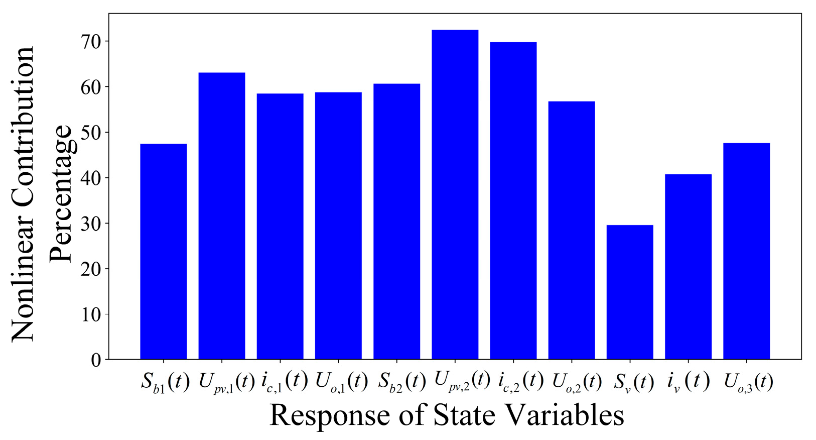
• Nonlinear Overall Contribution Index S_i

A novel nonlinear overall contribution index S_i is defined to quantify the magnitude of impact from nonlinear modal interactions on the system response, as shown in (14). Computed in MATLAB 2024a using pre-calculated excitation levels L_2i and N_2i (from Equations (9) and (10)), S_i for each response x_i is given by the ratio of the summed |N_2i| (composite-mode amplitude) to the total amplitude (sum of |N_2i| and ||L_2i||). The index further provides a holistic metric for characterizing the strength of nonlinearity in the system.

$$S_i={\displaystyle \frac{\left|N_{2i}\right|}{\left|L_{2i}\right|+\left|N_{2i}\right|}}={\displaystyle \frac{\left|{\displaystyle \sum _{j=1}^N{u}_{ij}}{\displaystyle \sum _{k=1}^N{\displaystyle \sum _{l=1}^N{h}_{2,kl}^j}}{y}_{k0}{y}_{l0}\right|}{\left|{\displaystyle \sum _{j=1}^N{u}_{ij}}{\displaystyle \sum _{k=1}^N{\displaystyle \sum _{l=1}^N{h}_{2,kl}^j}}{y}_{k0}{y}_{l0}\right|+\left|{\displaystyle \sum _{j=1}^N{u}_{ij}}\left(y_{j0}-{\displaystyle \sum _{k=1}^N{\displaystyle \sum _{l=1}^N{h}_{2,kl}^j}}{y}_{k0}{y}_{l0}\right)\right|}}$$

(14)

• Composite Mode Contribution Index I_r,kl

Composite modes are described by the interaction of two fundamental modes (e.g., λ_k + λ_l, k/l = 1, 2, …, N). The term N_2ikl (shown in (15)), which reflects the contribution of the composite mode formed by λ_k and λ_l to the response of the ith state variable, is decided by two parameters. The amplitude |N_2ikl| governs the peak response magnitude at t = 0. Meanwhile, the reciprocal of the real part of the eigenvalue sum τ_kl = −1/Re (λ_{k +} λ_l) defines the time constant which governs the decay rate of composite mode oscillations. By integrating both amplitude and temporal persistence of modal effects, based on [20], an innovative composite mode contribution index is proposed that incorporates an exponential function, as shown in Equation (16) (in this paper, β = 1.1).

$$N_{2ikl}={\displaystyle \sum _{j=1}^N{N}_{2i}}={\displaystyle \sum _{j=1}^N{u}_{ij}}{y}_{k0}{y}_{l0}{\mathrm{e}}^{\left({\lambda }_k+{\lambda }_l\right)t}$$

(15)

$$I_{r,kl}=\exp \left(\beta \cdot {\displaystyle \frac{|{\displaystyle \sum _{j=1}^N{u}_{ij}}{y}_{k0}{y}_{l0}|}{\mathrm{Re}\left({\lambda }_k+{\lambda }_l\right)}}\right)-1,\hspace{1em}\beta >0$$

(16)

This approach diverges from the traditional linear combination of amplitude and temporal persistence, which has been widely employed in previous studies. The introduction of the exponential function significantly enhances the sensitivity and discriminative power of the index, particularly in amplifying differences in modal contributions and capturing the nonlinear characteristics of composite mode interactions.

By quantifying the composite mode’s impact, facilitates the following:

• Post-disturbance Modal Analysis: Accurate identification of dominant modes critical for stability evaluation.
• Control Design Optimization: Prioritized selection of high-impact modes for strategic improvements.
• Predictive Modeling Enhancement: Comprehensive incorporation of intermodal interactions for precise system dynamic judgment.

To summarize, the analytical steps of the proposed framework are depicted in the flowchart shown in Figure 1.

3. Case Study

To validate the proposed analytical framework and indices, experimental verifications were conducted on a DC microgrid system and a PV system connected to the AC grid via a Boost converter and an inverter (PV DC-AC system). The results from both systems demonstrate the effectiveness of the proposed indices in capturing key dynamic characteristics and interactions, thereby confirming their applicability across diverse power systems.

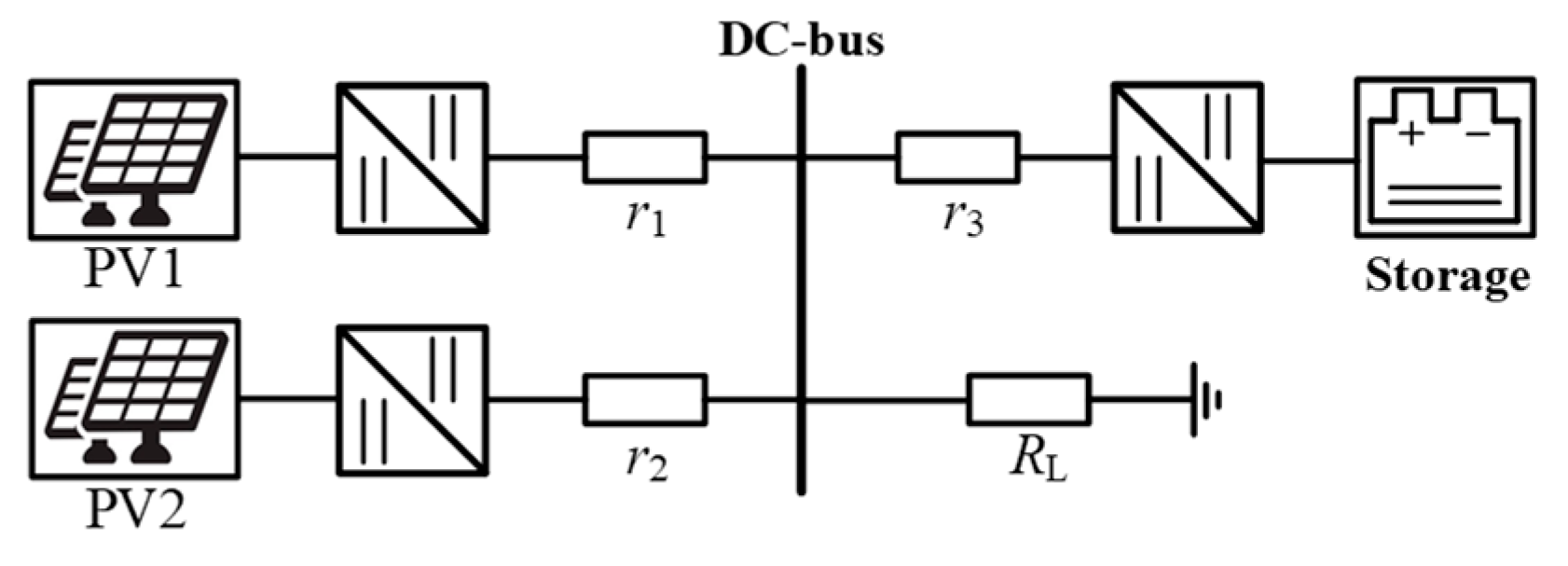
3.1. DC Microgrid System

3.1.1. System Modeling

In this section, a mathematical model of a three-unit PV-storage DC microgrid is established. The generation side comprises two PV modules and one energy storage module, while the load side is configured with an equivalent resistive load R_L. The system’s dynamic behavior is primarily governed by power electronic devices, with its topology illustrated in Figure 2.

The DC microgrid operates at a rated bus voltage of 300 V with an equivalent load of 1Ω. Two Kyocera KC200GT photovoltaic arrays ([21]) are implemented: array PV1 comprises six parallel strings, each with 20 series-connected modules; array PV2 comprises five parallel strings, each also with 20 series-connected modules.

Both modules operate under standard test conditions (STCs: 1 kW/m² irradiance, 25 °C ambient temperature). Control parameters for photovoltaic maximum power point tracking (MPPT) and energy storage regulation, along with detailed electrical specifications, are systematically documented in

Table 1. Photovoltaic module parameters.

Parameters		PV1	PV2
Filter	Cpv/mF	0.3	0.5
	Lc/mH	1.5	2
	Cc/mF	0.5	0.8
Line Resistance	r1,2/mΩ	0.4	0.5
Control System	kPc	0.05	0.05
	kIc	5	5

and

Table 2. Storage module parameters.

Parameters		Value	Parameters		Value
Filter	Cv/mF	3	Battery Voltage	Us/V	200
	Lv/mH	1.5	Control System	kPv	0.01
Voltage Reference	Uoref/V	300		kIv	10
Line Resistance	r3/mΩ	0.5		Rv	0.02

. The PWM sampling frequency in all three modules is 20 kHz.

Figure 3 depicts the circuit topology and hierarchical control architecture of the PV modules. The outer control loop, governed by MPPT algorithms, exhibits inherently slower dynamics compared to the inner current regulation loop due to its dependence on iterative power optimization processes. This temporal decoupling justifies the quasi-static assumption for outer-loop dynamics during transient stability analysis. Therefore, the mathematical model of the system can be derived as follows:

$$\left\{\begin{array}{l}{\displaystyle \frac{d{S}_{b,m}}{dt}}=k_{Ic,m}(U_{pvref,m}-U_{pv,m})\hfill \\ \begin{array}{l}{C}_{pv,m}{\displaystyle \frac{d{U}_{pv,m}}{dt}}=i_{pv,m}-i_{c,m}+S_{b,m}{i}_{c,m}+k_{Pc,m}(U_{pvref,m}-U_{pv,m})i_{c,m}\\ \hspace{1em}\hspace{1em}\hspace{1em}\hspace{1em}\end{array}\hfill \\ \begin{array}{l}{L}_{c,m}{\displaystyle \frac{d{i}_{c,m}}{dt}}=U_{pv,m}-U_{o,m}-S_{b,m}{U}_{pv,m}-k_{Pc,m}(U_{pv,m}^{\mathrm{ref}}-U_{pv,m})U_{pv,m}\\ \hspace{1em}\hspace{1em}\hspace{1em}\hspace{1em}\end{array}\hfill \\ C_{c,m}{\displaystyle \frac{d{U}_{o,m}}{dt}}=i_{c,m}-{\displaystyle \frac{U_{o,m}-{\displaystyle \sum _{i=1}^3{\alpha }_i}{U}_{o,i}}{r_m}}\hfill \end{array}\right.$$

(17)

where m = 1, 2 denotes the distinct PV modules, while i = 1, 2, 3 covers all modules, including the storage module (i = 3); U_pvref denotes the PV reference voltage set by the MPPT algorithm (see [21] for details); k_Pc,m and k_Ic,m are the PI controller parameters; U_o,i is the voltage at the ith node; r_i is the line resistance of the ith module; C_pv,m, L_c,m, and C_c,m are the corresponding filter parameters in the mth PV module; U_pv,m denotes the voltage across C_pv,m; S_b,m is the integral controller output; i_c,m is the current through L_c,m; R_L is the equivalent load resistance; α_i is the voltage distribution constant of the ith module, calculated as follows:

$${\alpha }_i={\displaystyle \frac{1/r_i}{1/R_L+1/r_1+1/r_2+1/r_3}}$$

(18)

Figure 4 depicts the energy storage module’s circuit topology and control strategy, with its mathematical model derived as follows:

$$\left\{\begin{array}{l}{\displaystyle \frac{d{S}_v}{dt}}=k_{Iv}(U_{oref}-U_{o,3})\hfill \\ \begin{array}{l}{L}_v{\displaystyle \frac{d{i}_v}{dt}}=U_s-U_{o,3}+S_v{U}_{o,3}+k_{Pv}(U_{oref}-U_{o,3})U_{o,3}-R_v{i}_v{U}_{o,3}\\ \hspace{1em}\hspace{1em}\hspace{1em}\end{array}\hfill \\ C_v{\displaystyle \frac{d{U}_{o,3}}{dt}}=i_v-S_v{i}_v-k_{Pv}(U_{oref}-U_{o,3})i_v+R_v{i}_v^2-{\displaystyle \frac{U_{o,3}-{\displaystyle \sum _{i=1}^3{\alpha }_i}{U}_{o,i}}{r_3}}\hfill \\ \hspace{1em}\hspace{1em}\hspace{1em}\hfill \end{array}\right.$$

(19)

where S_v is the integral controller output; k_Pv and k_Iv are the parameters of the PI controller; R_v is the active damping coefficient; U_s is the terminal voltage of the battery; U_oref is the DC-bus voltage reference; L_v and C_v are the corresponding filter parameters in the storage module; i_L is the current through L_v.

By integrating Equations (17) and (19), the 11th-order mathematical model of the DC microgrid can be derived. In addition, this modeling approach can be generalized to an n-machine AC/DC system.

3.1.2. Result Analysis

Building upon the established mathematical models, this section systematically examines how variable interactions influence the dynamic behavior of the DC microgrid system by applying the proposed analytical framework.

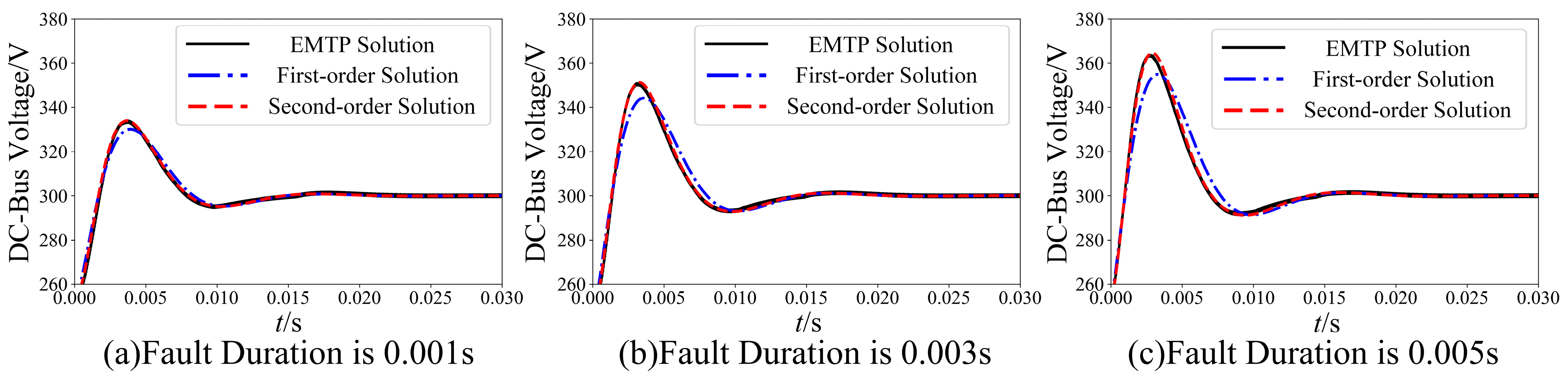
• Accuracy Analysis of Analytical Solutions

To demonstrate the characteristic nonlinear dynamics inherent in DC microgrid systems, we conducted a nonlinearity assessment through Equation (14), with computational results as detailed in Figure 5. The analysis reveals that nonlinear components contribute over 30% to the response characteristics across all state variables. This empirical evidence demonstrates that conventional linearized first-order analytical approaches are inadequate to characterize system dynamics. Therefore, implementing second-order nonlinear analytical solutions is essential for an accurate representation.

This section employs simulation experiments to systematically examine transient responses of nonlinear systems under diverse fault conditions. The experimental protocol initializes system state variables using post-fault clearance instantaneous values, followed by the computational derivation of first- and second-order analytical solutions. Through comparative analysis with EMTP-generated numerical solutions (Figure 6, Figure 7 and Figure 8), we establish solution accuracy under two operational scenarios:

• Constant fault severity with variable duration (Figure 6 and Figure 7);
• Fixed duration with varying severity (Figure 8).

The results demonstrate that increased fault duration/intensity amplifies system disturbances, degrading both solution accuracies, while second-order solutions exhibit markedly enhanced descriptive capacity, as evidenced by the reduced waveform deviations in (Figure 6, Figure 7 and Figure 8). This empirical evidence confirms the second-order nonlinear solution’s enhanced capability in capturing system dynamics.

For quantitative precision assessment, we implemented error metrics from Equations (20) and (21) through comparative waveform analysis with EMTP benchmarks (

Table 3. Calculation errors in the system response solution.

Disturbance Magnitude/%	2.34	5.305	7.162	12.833
First-order Error/%	9.523	11.506	14.046	15.879
Second-order Error/%	3.856	5.221	6.284	7.539
Disturbance Magnitude/%	15.253	18.985	23.418	25.524
First-order Error/%	20.682	22.789	26.357	30.143
Second-order Error/%	12.233	14.755	19.406	24.484

). Experimental data spanning disturbance magnitudes from 2.34% to 25.524% demonstrate that first-order solutions exhibit error margins between 9.523% and 30.143%, while second-order counterparts maintain significantly reduced errors ranging from 3.856% to 24.484%. These findings necessitate the critical adoption of second-order solutions during nonlinear system transients, as their enhanced nonlinear structural representation provides more accurate response characterization and deeper system insight.

$$E_m=\sqrt{{\displaystyle \frac{{\displaystyle \sum {\left|\left(X_0\left(t_n\right)-X_i\left(t_n\right)\right)\right|}^2}}{{\displaystyle \sum {\left|X_0\left(t_n\right)\right|}^2}}}}\times 100\%$$

(20)

$$E=(1/N){\displaystyle \sum _{m=1}^N{E}_m}$$

(21)

where X₀ (t_n) and X_i (t_n) (i = 1, 2) represent the values at time t_n from the EMTP simulation results, the first-order solution, and the second-order solution, respectively.

2.

Analysis of the Impact of Nonlinear Modal Interaction on System Response

Table 4. Fundamental modes and the corresponding fundamental modal influence index under varying disturbance magnitudes.

Fundamental Modal Number	Eigenvalue	State Variable with High Degree of Participation	Disturbance Magnitude 5.305/%		Disturbance Magnitude 15.253/%		Disturbance Magnitude 20.524/%
			|I1,j|/p.u.	θj/rad	|I1,j|/p.u.	θj/rad	|I1,j|/p.u.	θj/rad
λ1,2	−2512.83 ± 2791.91i	Upv,1, ic,1	1.0402	∓0.4127	1.0446	∓0.4734	1.0011	∓0.2400
λ3	−4141.43	Uo,1	1.6349		2.2721		2.3929
λ4,5	−3084.30 ± 1831.27i	Upv,2, ic,2	2.0029	∓0.6730	2.9383	∓1.0300	2.3255	∓1.3313
λ6,7	−1782.69 ± 230.847i	Uo,2, iv, ic,2	1.1911	±1.5024	2.5805	±1.9125	4.0171	±1.9594
λ8,9	−124.617 ± 570.608i	Sv, iv, Uo,3	1.0481	±0.0222	1.0209	±0.0658	0.9734	±0.1225
λ10	−48.332	Sb1	0.9473		0.9138		0.8832
λ11	−98.630	Sb2	0.8881		0.7992		0.7023

documents the system’s fundamental oscillation modes, accompanied by their dominant participating state variables (ranked through participation factor magnitudes) and corresponding first-order modal influence index I_1j derived from (13).

The comparative analysis reveals that intermodal coupling induces substantial disparities between first- and second-order solutions, mainly manifested through:

• Divergent initial amplitude-phase characteristics of identical modes;
• Distinct state transition patterns;
• Non-negligible variations in dynamic response signatures.

As shown in Table 4, when the disturbance magnitude is fixed at 15.253%, systematic examination of initial amplitude distribution reveals that nonlinear intermodal couplings can significantly amplify the initial amplitudes of specific fundamental modes, particularly modes 1 (2), 3, 4 (5), 6 (7), and 8 (9). Conversely, these nonlinear interactions demonstrate amplitude suppression effects on modes 10 and 11. This phenomenon indicates that secondary modes identified in linear first-order analysis may evolve into principal dynamic contributors through nonlinear coupling mechanisms. Such findings necessitate paradigm shifts in theoretical modeling and control strategy development for complex dynamical systems.

Additionally, the relationship between first-order fundamental modal influence indices and disturbance amplitude reveals characteristic extremal behavior. Under varying excitation levels, specific modal groups (e.g., λ₄ and λ₅) exhibit distinct peak/trough response patterns in their oscillation magnitudes. The disturbance-magnitude-governed nonlinearity induces complex intermodal energy transfers characterized by excitation-dependent non-monotonic coupling responses.

Detailed investigation of control-critical modes (8, 9, 10, 11) demonstrates progressive degradation of disturbance responsiveness with increasing excitation amplitude. When exceeding the critical controllability threshold, control implementations fail to compensate for the amplified nonlinear coupling effects, ultimately destabilizing the system. This amplitude-dependent controllability degradation highlights how inherent nonlinearities fundamentally constrain control authority in dynamical systems. Consequently, controller synthesis and parameter optimization must systematically incorporate these nonlinear characteristics through rigorous mathematical modeling and stability analysis.

The DC bus voltage serves as a critical stability indicator in the system, with its transient response characteristics being particularly vital for operational integrity. Investigating nonlinear inter-variable coupling effects on DC bus voltage dynamics (U_o3) holds significant research value, serving dual purposes: both deepening fundamental insights into stability mechanisms and providing theoretical underpinnings for optimizing control strategies. As demonstrated in Figure 9, the comparative analysis contrasts the oscillatory dynamics of fundamental mode 4 (5) in the U_o3 response between first-order and second-order solutions. The comparative results reveal divergent dynamic manifestations of identical fundamental modes across different solution approaches.

This solution-dependent discrepancy primarily stems from nonlinear intermodal coupling effects that substantially modify both amplitude modulation and phase initialization characteristics. Under particular operational regimes, these nonlinear interactions may induce critical phase anomalies exceeding 90° deviations, potentially resulting in complete phase inversion phenomena. Such nonlinear phase-amplitude modulation effects represent a crucial consideration in modern power system analysis, imperative for maintaining stability margins and ensuring controller efficacy in practical implementations.

Based on Equations (10) and (15), the composite mode contribution index is computed to characterize modal excitation states, with results documented in

Table 5. Results of modal nonlinearity contribution factors of DC-bus voltage response.

Fundamental Mode Pair (λk + λl)	Eigenvalue Sum	N2,ikl		Ir,kl
		Amplitude/V	Amplitude Percentage/p.u.
8 + 8	−249.3 + 1141.0i	10.638	18.09	0.0481
9 + 9	−249.3 − 1141.0i
7 + 8	−1906.0 + 338.5i	27.734	47.17	0.0161
6 + 9	−1906.0 − 338.5i
8 + 9	−249.3	1.711	2.90	0.0076
6 + 8	−1906.0 + 802.8i	11.526	19.60	0.0067
7 + 9	−1906.0 − 802.8i
6 + 7	−3563	5.163	8.78	0.0016
6 + 6	−3563.0 + 464.2i	2.021	3.44	0.00063
7 + 7	−3563.0 − 464.2i

. Adopting an excitation threshold criterion of 0.01 p.u. response amplitude for composite mode significance filtering, the analysis reveals that dominant composite modes predominantly originate from two distinct intramodal coupling mechanisms, as listed in the first column of Table 5:

• Cross-coupling between fundamental modes through pairwise combinations (e.g., λ₆ + λ₇, λ₇ + λ₈, λ₈ + λ₉)
• Self-coupling phenomena where individual modes interact with themselves (e.g., λ₈ + λ₈, λ₉ + λ₉)

Further analysis of DC bus voltage output dynamics reveals intense coupling among modes λ₆, λ₇, λ_8, and λ₉, which directly manifests as strong cross-module interactions between photovoltaic module 2 (PV2) and the energy storage module. In contrast, photovoltaic module 1 (PV1) exhibits independent dynamic characteristics unaffected by these modal interactions. This operational dichotomy necessitates explicit consideration of modal coupling effects between λ₆, λ₇, λ_8, and λ₉ during stability analysis and control law synthesis for optimal dynamic performance management.

To validate the conclusions above, trajectory sensitivity analysis was implemented to quantify the dynamic coupling effects between PV modules and the energy storage system. While incapable of capturing nonlinear multi-timescale dynamics, trajectory sensitivity’s parametric sensitivity metrics directly corroborate modal energy transfer patterns, resolving temporal coupling intensity for hypothesis verification. To ensure the validity of sensitivity comparisons, PV1 and PV2 controllers were designed with identical PI structures and bandwidth specifications (shown in Table 1). As demonstrated in Figure 10 (adopting the quantitative trajectory sensitivity calculation methodology from [22]), the PI control parameters (k_Pc and k_Ic) in PV2 exhibit significantly higher trajectory sensitivity magnitudes (1.58 and 0.42 p.u.) on DC bus voltage U_o3 compared to those in PV1 (0.51 and 0.09 p.u.) throughout the 0~0.04 s transient period. This order-of-magnitude disparity in sensitivity coefficients explicitly corroborates the previously identified operational dichotomy: PV2′s control dynamics demonstrate stronger parametric interdependence with the energy storage module’s operational states, while PV1 maintains essentially decoupled regulation characteristics, which substantiate the theoretical framework’s predictive capability in mapping cross-module dynamic interactions through modal coupling signatures.

Comprehensive spatiotemporal analysis integrating composite mode contribution index I_r,kl (calculated from Equation (15)) establishes the self-interaction modes of λ₈ + λ₈ and λ₉ + λ₉ as pivotal regulators of DC voltage response characteristics. Their operational dominance stems from a dual-aspect coupling mechanism: (1) nonlinear interaction between the Boost converter’s reference-tracking switching dynamics; (2) energy buffering dynamics in the storage subsystem’s capacitive elements.

This coupling architecture facilitates DC bus voltage regulation through sequential energy conversion processes:

• Reference voltage deviations activate Boost switching adjustments;
• Switching transients directly excite modes λ₈ + λ₉ through inductor-capacitor resonance;
• Modal energy redistribution stabilizes DC voltage fluctuations.

The demonstrated control-to-modal transduction hierarchy confirms the energy storage subsystem’s role as the principal architect of system dynamics, requiring specialized stability criteria for microgrid configurations.

The above analysis indicates that the dynamic behavior of DC microgrids is influenced not only by individual module controls but also critically constrained by nonlinear couplings between photovoltaic arrays, energy storage systems, and DC network parameters. These interaction mechanisms, particularly those mediated through modal coupling effects between λ₆, λ₇, λ_8, and λ₉, necessitate control strategy designs that systematically address both component-level dynamics and cross-module energy transfer characteristics. Critical implementation requirements should include adaptive compensation for modal coupling intensities and stability margin calibration under multi-modal operation.

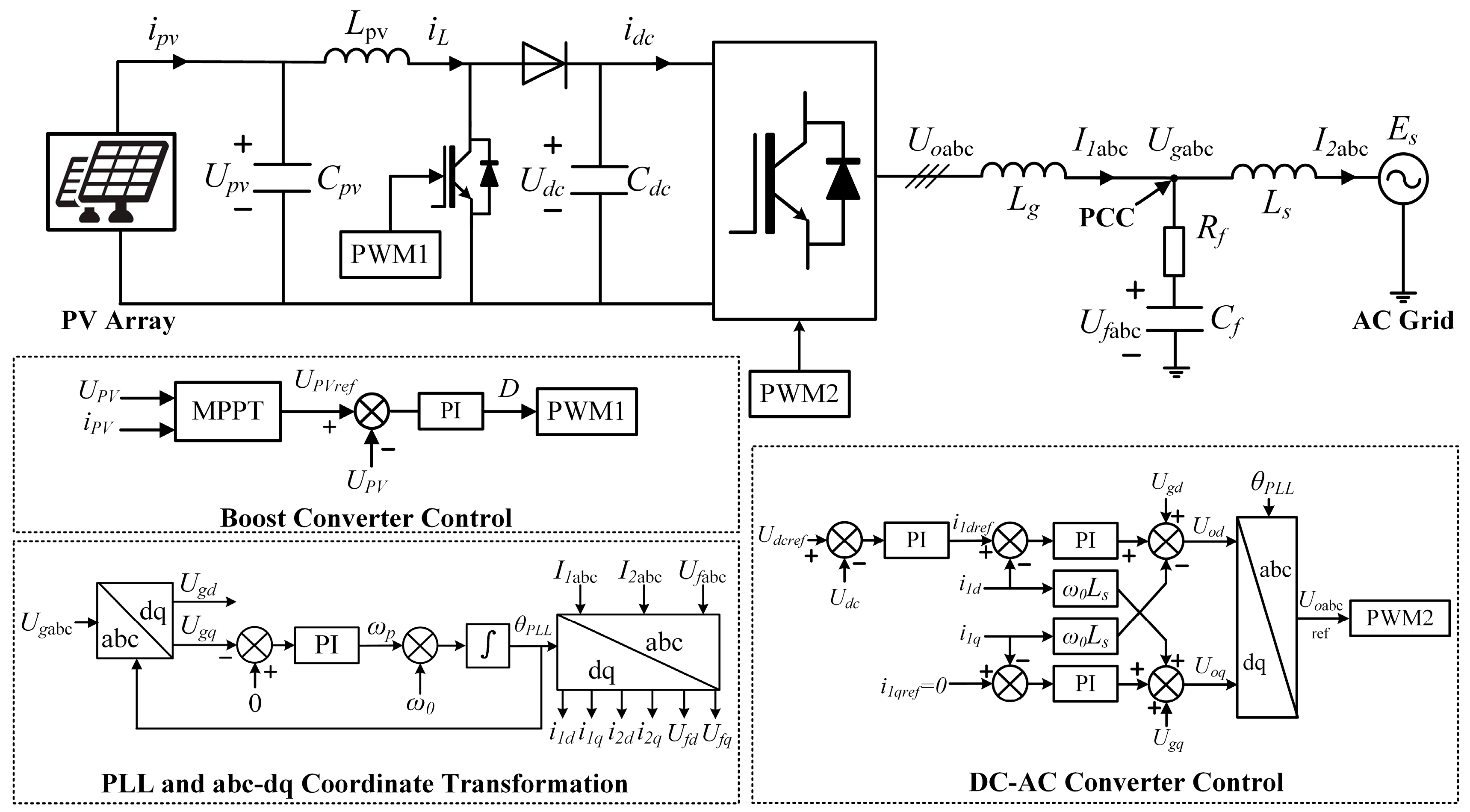
3.2. PV DC-AC System

To validate the applicability of the proposed framework to complex renewable energy systems, a grid-connected PV system, which integrates a boost DC-DC converter and a DC-AC inverter, is employed as a case study. The circuit topology and hierarchical control architecture of the system are depicted in Figure 11. Additionally, to further substantiate the experimental validation, a physical prototype of the PV DC-AC system was constructed and tested. The physical setup, including the interconnections between the components, is illustrated in Figure 12. The PV array is the Zhongfu Energy CM230P/CM260P Series. The boost converter function is implemented using the HZD-816 module. The inverter is a TS100KTL model. The control parameters of the DC-DC and DC-AC converters can be adjusted via accompanying software, facilitating a modular approach to system configuration and control. The AC-side LCL filter and the infinite bus grid are simulated using the Yanxu YXACS-YZ Series High-Power Regenerative AC Source and Load Integrated Grid Simulator.

The modeling process commences with the derivation of nonlinear equations that characterize the system dynamics, with detailed formulations provided in Appendix A. The state variables encompass:

• PV/DC Stage: x_pv (boost converter integral control output); U_pv (PV array voltage); i_L (L_pv inductor current), U_dc (DC-link voltage).
• AC Stage: i_1d, i_1q (inverter-side dq current); i_2d, i_2q (grid-side dq current); U_fd, U_fq (C_f filter capacitor voltage).
• Control States: θ_PLL (PLL output angle); x_dc (outer-loop DC voltage control integral state); x_id, x_iq inner-loop current control integral state.

The MSM is subsequently employed to obtain first-order and second-order approximations of the system response. A three-phase short-circuit fault was applied at the point of common coupling (PCC) with fault duration t_c of 0.1 s, 0.3 s, and 0.6 s. The dynamic evolution of the DC-link voltage, as predicted by both the first-order and second-order analytical solutions, was compared with the corresponding physical experimental waveforms, as illustrated in Figure 13. It is noteworthy that increasing fault duration (e.g., 0.6 s vs. 0.1 s) reduces the post-fault disturbance magnitude. This occurs because sustained faults allow the system to adapt to near-zero voltage, enabling controllers (DC voltage, current tracking, PLL) to dissipate transient energy and reach a stable quasi-steady state. Consequently, when the fault clears, recovery starts from this adapted state, minimizing initial deviations and DC-link voltage oscillations.

As demonstrated in Figure 13, the second-order solution exhibits significantly superior descriptive capacity for system dynamics compared to the first-order solution, with closer alignment to the physical experimental waveforms. The waveform deviations are notably reduced, with errors decreasing by 2.17~12.67% (calculated from (20)) across various fault duration times, confirming the enhanced ability of the second-order solution to capture nonlinear transient characteristics. This validation indicates that the improved modeling fidelity observed in the aforementioned DC microgrid system also extends to complex, DC-AC photovoltaic installations.

However, it is observed that the peak response of the second-order solution consistently exhibits a temporal lag of approximately 10 ms relative to the physical experimental waveforms. This temporal lag fundamentally originates from the equivalent damping effects introduced by the quadratic terms in the Taylor expansion. This phenomenon is particularly evident in the DC voltage dynamics governed by Equation (A4), where the nonlinear term 1/U_dc is expanded to the second order around the equilibrium point U_dc0. Specifically, during fault recovery when U_dc changes rapidly, this term acts as a virtual resistance that opposes the voltage increase, thereby reducing the magnitude of dU_dc/dt during the transient phase. This effect introduces a time delay, contributing to the observed temporal lag.

Subsequently, the composite mode contribution index I_r,kl from (15) is utilized to analyze the state variable interaction phenomenon in the DC-link voltage dynamic response during a three-phase short with a duration of 0.1 s, with the results presented in

Table 6. Results of modal nonlinearity contribution factors of DC-link voltage response.

Fundamental Mode Pair (λk + λl)	State Variable with High Degree of Participation	N2,ikl		Ir,kl
		Amplitude/V	|Re(λk + λl)|
9 + 9/10 + 10	Udc, xdc	14.34	114.42	0.1478
5 + 9/6 + 10	Udc, xdc, i1d, i1q, i2d, i2q	8.21	382.53	0.0239
5 + 10/6 + 9		7.14	382.53	0.0207
5 + 14/6 + 15	i1d, i1q, i2d, i2q, Ufd, Ufq	2.19	621.36	0.0039
5 + 15/6 + 14		1.12	621.36	0.0020

.

From Table 6, we can derive the following conclusions:

• DC-Link Voltage Control Dominance: Modal analysis shows that the most influential mode involves the DC-link voltage (U_dc) and its integral controller state (x_dc). This mode dominates transient responses during PCC faults due to its role in power balance regulation. The sudden loss of AC power output rapidly charges C_dc, while the PI controller (k_pdc, k_idc) struggles to restore equilibrium.
• Critical Converter Current Coupling: The secondary dominant mode links U_dc with converter-side dq-currents (i_1d, i_1q). This reflects the interaction between DC-link dynamics and the inverter’s power injection capability.
• Significant PCC/Filter Network Dynamics: The third major mode encompasses PCC currents (i_2d, i_2q), filter voltages (U_fd, U_fq), and converter currents (i_1d, i_1q). It captures the interaction between the LCL filter’s resonant dynamics and fault-induced voltage collapse at the PCC.
• Negligible PV/Boost Dynamics and Model Reduction Opportunity: Photovoltaic states (x_PV, U_PV) and boost converter variables (i_L) are absent from dominant modes. PV-side dynamics have minimal influence on fault-induced DC transients due to the slow response of the PV system. Consequently, the PV generation and DC-DC conversion stage can be simplified to a constant power source (P_PV) or an ideal current source (i_PV ≈ const) for fault stability studies, reducing computational complexity while preserving accuracy in modeling critical DC-AC interactions.

4. Conclusions

This study establishes a unified framework for quantifying nonlinear interactions in power electronics-dominant systems, integrating second-order analytical solutions with composite modal indices. Validation across a DC microgrid system and a PV grid-connected system confirms the framework’s universality. Key advances are synthesized as follows:

• System Nonlinear Dynamics
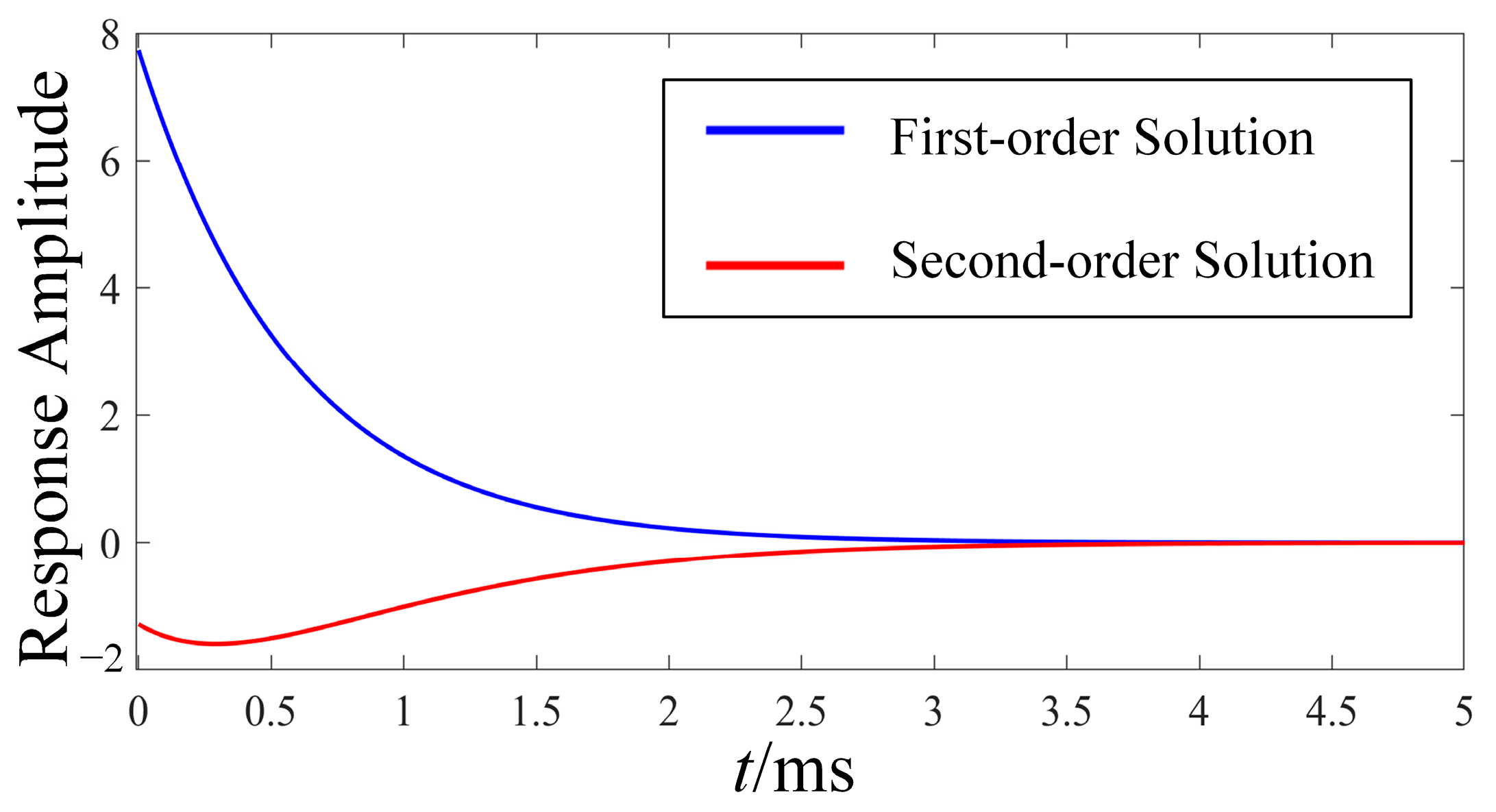
  • Second-order solution superiority: Accurately captures multi-mode oscillations/damping distortion under 5~15% disturbances, outperforming linearization—critical for modeling fault-induced transients like rapid DC-link capacitor charging during PCC faults.
  • Modal dominance inversion: Nonlinear coupling induces amplitude/phase modifications in fundamental modes, potentially reversing modal dominance hierarchies identified through linear methods.
  • Composite mode emergence: Specific fundamental mode combinations (e.g., modes λ₆, λ₇, λ_8, and λ₉ in the DC microgrid system) generate composite modes that critically govern system output characteristics.
• Critical Interaction Mechanisms
  • DC Microgrid Voltage Regulation: Composite modes formed by λ₈ + λ₈ and λ₉ + λ₉ regulate DC voltage through dual mechanisms: (1) boost converter switching excites LC resonance to activate modal responses, and (2) storage capacitor buffering enables energy redistribution for stabilization.
  • PV System Fault Dynamics: Three dominant interactions govern PCC faults: (1) U_dc-x_dc coupling maintains power balance, (2) U_dc-i_1d/i_1q synergy constrains inverter current capability, (3) LCL filter resonance (i_2d/i_2q-U_fd/U_fq-i_1d/i_1q) drives voltage collapse.
• Design Implications And Scalability
  • Control System Synthesis: Requires amplitude-aware compensation for modal clusters (e.g., modes λ₆, λ₇, λ_8, and λ₉ in DC microgrid system) and adaptive gain scheduling for DC-AC converter current coupling.
  • Model Reduction: PV array and Boost converter dynamics (x_PV, U_PV, i_L) are negligible during faults, enabling replacement with constant power sources.

References

1. IRENA. Global Renewables Outlook: Energy Transformation 2050, 2020th ed.; International Renewable Energy Agency: Abu Dhabi, United Arab Emirates, 2020. [Google Scholar]
2. Lew, D.; Bartlett, D.; Groom, A.; Jorgensen, P.; O’sUllivan, J.; Quint, R.; Rew, B.; Rockwell, B.; Sharma, S.; Stenclik, D. Secrets of Successful Integration: Operating Experience With High Levels of Variable, Inverter-Based Generation. IEEE Power Energy Mag. 2019, 17, 24–34. [Google Scholar] [CrossRef]
3. Jiang, Q.; Wang, Y. Overview of the Analysis and Mitigation Methods of Electromagnetic Oscillations in Power Systems With High Proportion of Power Electronic Equipment. J. Proc. CSEE 2020, 40, 7185–7201. [Google Scholar] [CrossRef]
4. Alam, S.; Al-Ismail, F.S.; Salem, A.; Abido, M.A. High-Level Penetration of Renewable Energy Sources Into Grid Utility: Challenges and Solutions. IEEE Access 2020, 8, 190277–190299. [Google Scholar] [CrossRef]
5. Shu, D.; Xie, X.; Rao, H.; Gao, X.; Jiang, Q.; Huang, Y. Sub- and Super-Synchronous Interactions Between STATCOMs and Weak AC/DC Transmissions With Series Compensations. IEEE Trans. Power Electron. 2018, 33, 7424–7437. [Google Scholar] [CrossRef]
6. Liu, Y.; Shuai, Z.; Li, Y.; Cheng, Y.; Shen, Z. Harmonic Resonance Modal Analysis of Multi-inverter Grid-connected Systems. J. Proc. CSEE 2017, 37, 4156–4164+4295. [Google Scholar] [CrossRef]
7. Hasan, K.N.M.; Rauma, K.; Luna, A.; Candela, J.I.; Rodriguez, P. Study on harmonic resonances and damping in wind power plant. In Proceedings of the 2012 4th International Conference on Intelligent and Advanced Systems (ICIAS2012), Kuala Lumpur, Malaysia, 12–14 June 2012; pp. 418–423. [Google Scholar] [CrossRef]
8. Hong, L.; Shu, W.; Wang, J.; Mian, R. Harmonic Resonance Investigation of a Multi-Inverter Grid-Connected System Using Resonance Modal Analysis. IEEE Trans. Power Deliv. 2019, 34, 63–72. [Google Scholar] [CrossRef]
9. Tahim, A.P.N.; Pagano, D.J.; Lenz, E.; Stramosk, V. Modeling and Stability Analysis of Islanded DC Microgrids Under Droop Control. IEEE Trans. Power Electron. 2015, 30, 4597–4607. [Google Scholar] [CrossRef]
10. Anand, S.; Fernandes, B.G. Reduced-Order Model and Stability Analysis of Low-Voltage DC Microgrid. IEEE Trans. Ind. Electron. 2013, 60, 5040–5049. [Google Scholar] [CrossRef]
11. Marx, D.; Magne, P.; Nahid-Mobarakeh, B.; Pierfederici, S.; Davat, B. Large Signal Stability Analysis Tools in DC Power Systems with Constant Power Loads and Variable Power Loads—A Review. IEEE Trans. Power Electron. 2012, 27, 1773–1787. [Google Scholar] [CrossRef]
12. Kabalan, M.; Singh, P.; Niebur, D. Large Signal Lyapunov-Based Stability Studies in Microgrids: A Review. IEEE Trans. Smart Grid 2017, 8, 2287–2295. [Google Scholar] [CrossRef]
13. Sanchez-Gasca, J.; Vittal, V.; Gibbard, M.; Messina, A.; Vowles, D.; Liu, S.; Annakkage, U. Inclusion of higher order terms for small-signal (modal) analysis: Committee report-task force on assessing the need to include higher order terms for small-signal (modal) analysis. IEEE Trans. Power Syst. 2005, 20, 1886–1904. [Google Scholar] [CrossRef]
14. Thapar, J.; Vittal, V.; Kliemann, W.; Fouad, A. Application of the normal form of vector fields to predict interarea separation in power systems. IEEE Trans Power Syst. 1997, 12, 844–850. [Google Scholar] [CrossRef]
15. Pariz, N.; Shanechi, H.; Vaahedi, E. Explaining and validating stressed power systems behavior using modal series. IEEE Trans. Power Syst. 2003, 18, 778–785. [Google Scholar] [CrossRef]
16. Shanechi, H.; Pariz, N.; Vaahedi, E. General nonlinear modal representation of large scale power systems. IEEE Trans. Power Syst. 2003, 18, 1103–1109. [Google Scholar] [CrossRef]
17. Wu, F.; Wu, H.; Han, Z.; Gan, D. Comparison between methods for power system nonlinear modal analysis. J. Proc. CSEE 2007, 34, 19–25. [Google Scholar]
18. Rodríguez, O.; Medina, A.; Andersson, G. Closed-form analytical characterisation of non-linear oscillations in power systems incorporating unified power flow controller. IET Gener. Transm. Distrib. 2015, 9, 1019–1032. [Google Scholar] [CrossRef]
19. Zhang, H.; Yi, C.; Wei, T. Non-linear modal analysis of transient interaction behaviours in SEPIC DC–DC converters. IET Power Electron. 2017, 10, 1190–1199. [Google Scholar] [CrossRef]
20. Zeinali, R.; Ghazi, R.; Pariz, N. Nonlinear interaction problems of large capacity wind farms. In Proceedings of the Iranian Conference of Smart Grids, Tehran, Iran, 24–25 May 2012; pp. 1–6. [Google Scholar]
21. Villalva, M.G.; Gazoli, J.R.; Filho, E.R. Comprehensive Approach to Modeling and Simulation of Photovoltaic Arrays. IEEE Trans. Power Electron. 2009, 24, 1198–1208. [Google Scholar] [CrossRef]
22. Buragohain, U.; Mir, A.S.; Senroy, N. Transient Stability Assessment of a DFIG-WTG System Using Trajectory Sensitivity Analysis. IEEE Trans. Power Syst. 2024, 39, 5818–5828. [Google Scholar] [CrossRef]
Figure 1. Flowchart of the proposed framework.
Electronics 14 02902 g001
Figure 2. Circuit topology of a three-machine photovoltaic storage DC microgrid.
Electronics 14 02902 g002
Figure 3. Circuit topology and control strategies of the photovoltaic module.
Electronics 14 02902 g003
Figure 4. Circuit topology and control strategies of the storage module.
Electronics 14 02902 g004
Figure 5. Calculation results of the system’s nonlinearity degree.
Electronics 14 02902 g005
Figure 6. Comparison of three waveforms under varying fault durations with a 30% load decrease.
Electronics 14 02902 g006
Figure 7. Comparison of three waveforms under varying fault durations with a 30% load increase.
Electronics 14 02902 g007
Figure 8. Comparison of three waveforms under identical fault duration time with varying degrees of fault severity.
Electronics 14 02902 g008
Figure 9. Curves of mode 4 (5) in DC-bus voltage response.
Electronics 14 02902 g009
Figure 10. Trajectory sensitivity waveform of DC bus voltage.
Electronics 14 02902 g010
Figure 11. Circuit topology and control strategies of the PV DC-AC system.
Electronics 14 02902 g011
Figure 12. Illustrative schematic of the PV DC-AC system setup.
Electronics 14 02902 g012
Figure 13. Comparison of three waveforms under three-phase short circuits with different varying fault durations.
Electronics 14 02902 g013