An Efficient Malware Detection Method Using a Hybrid ResNet-Transformer Network and IGOA-Based Wrapper Feature Selection

Abstract

The growing sophistication of malware and other cyber threats presents significant challenges for detection and prevention in modern cybersecurity systems. In this paper an efficient and novel malware classification model using the Hybrid Resnet-Transformer Network (HRT-Net) and Improved Grasshopper Optimization Algorithm (IGOA) is proposed. Convolutional layers in the resnet50 model effectively extract local features from malware patterns, while the Transformer focuses on long-range dependencies and complex patterns by leveraging multi-head attention. The extracted local and global features are concatenated to create a rich feature representation, enabling precise malware detection. The Improved Grasshopper Optimization Algorithm with dynamic mutation coefficient and dynamic inertia motion weights is employed to select an optimal subset of features, reducing computational complexity and enhancing classification performance. Finally, the Ensemble Learning technique is used to robustly classify malware samples. Experimental evaluations on the Malimg dataset demonstrate the high efficiency of the proposed method, achieving an impressive accuracy of 99.77%, which shows greater efficiency compared to other recent studies.

1. Introduction

Malware is a shortened term for malicious software, which is any kind of software that is designed to be used for a malicious purpose and to disrupt the operations of a computer and/or its users. There are many different types of malware, some of which are computer viruses [1], rootkits [2], worms [3], backdoors [4], Trojan horses [5], spyware [6], scareware [7], botnets [8], and intrusive adware [9]. They are able to perform delete operations that threaten the confidentiality, integrity, and availability of computer systems. As computing capabilities are rapidly improving and the integration of computerized systems is becoming deeper, malware has become one of the most significant threats to the world [10]. Although the use of the Internet remains an essential part of modern day life in that it supports activities such as electronic commerce [11], banking [12], real-time communication [13], and entertainment [14], it has given rise to new and continuously emerging threats posed by the malware that makes digital systems’ private, reliable, and accessible. As a result, malwares designed for both Android and Windows platforms have posed security risks to Internet users. Cybercriminals strategically utilize malware on Windows and Android operating systems to achieve diverse malicious aims, including the unauthorized exfiltration of user data, identity fraud, and various other illicit operations [15]. Several approaches to malware detection have been mentioned in the literature, and one of the most widely used is signature-based detection (also referred to as known malware pattern detection). However, this approach cannot detect new and even modified versions of malware and thus is not sufficient when it comes to novel threats.

To overcome these limitations, other research has been carried out which pointed to the dynamic analysis of an application where traces of execution and system calls are created. While these approaches provide improved means in analyzing the behavior of malware, they also present problems with reference to the monitoring at runtime. In this respect, deep learning has been under consideration as a more viable solution. While with the traditional machine learning strategies, it is necessary to hand-craft feature representation from the raw data, this is not the case with deep learning models, as these models are capable of learning feature extraction on their own. In recent years, there has been a shift towards the usage of deep learning for the detection of malware because of the availability of computing tools and complex neural networks [16].

While deep learning performs well in malware detection, relying only on a single type of deep network architecture may hinder the performance of the model when it comes to detecting hierarchical patterns in the malware dataset. The aims and purposes of feature extraction imply that different architectures are well suited to perform different aspects of feature extraction. While convolutional neural networks (CNNs), for example, are able to detect the local and spatial connections, Transformer-based networks are more suitable for learning long-range connections and contexts based on the self-attention mechanism. Therefore, the combination of these capabilities, within a common framework, can make for a gross improvement of the resilience and genericity of malware detection systems.

In recent years, there has been a rise in the use of hybrid deep learning architectures within the context of cybersecurity because of their efficiency in joining the features of various structures. These models not only improve the ability of the learning system in representing new inputs but also overcome the problems related to the sole application of the networks. In malware detection techniques, structures are sometimes concealed and multivariate; thus, a two-phase detector is able to capture a more comprehensive view from the resultant spatial features and temporal correlation professed in the dataset. Moreover, combining the hybrid feature extraction models with the smart selection of the features prevents the utilization of a number of features that are not relevant to the classification problem, which leads to both an overfitting and an increased computational load.

In the context of this paper, a novel approach based on the Hybrid ResNet-Transformer Neural Network (HRT-Net) is proposed to perform efficient and effective malware detection. To enhance the capabilities of the system, the current model combines the effectiveness of convolutional and Transformer networks. In particular, ResNet is designed to identify local features, which allows for a more accurate identification of existing patterns within the data of malware. At the same time, the Transformer component performs the same in terms of capturing the global dependency using the attention mechanism which aligns well with the relationships within the malware patterns. With the combination of the local and global features which are extracted separately by the proposed HRT-Net, the feature space of the model becomes larger and more detailed than before, which makes it improve the discriminative ability of the model. This new feature extraction approach has several technical benefits over the conventional feature extraction techniques. This is because HRT-Net incorporates both local and global features, enabling it to recognize complex patterns of malwares that other autonomous deep networks cannot detect. Further, the present method involves the use of the wrapper-based feature selection method with the Improved Grasshopper Optimization Algorithm (IGOA). The latest enhancement of the Grasshopper Optimization Algorithm, IGOA includes dynamic inertial motion weights, and applies a dynamic mutation coefficient that minimizes convergence to local optima to select an optimal feature subset in the context of malware detection systems. This optimal feature subset is then passed to the Ensemble Learning classifier to enhance high accuracy for the detection of malware. Not only does this reduce computational cost but it also increases the accuracy of the detection, hence making this method better than the existing methods in the analysis of malware.

Our contributions in this work are as follows:

• Introduction of a novel deep neural network, HRT-Net, designed to simultaneously extract both local and global features from malware images, resulting in a comprehensive and enriched representation of complex patterns and previously unknown threats.
• Utilization of a Multi-Head Attention mechanism within the Transformer module to identify long-range dependencies, high-level patterns, and semantic relationships within malware data, which significantly enhances detection accuracy.
• Implementation of a wrapper-based feature selection method employing the Improved Grasshopper Optimization Algorithm (IGOA), capable of identifying relevant features while eliminating redundant ones, thereby reducing inter-feature redundancy and improving model efficiency.
• Introducing an efficient and novel dynamic optimization technique, defined as Improved Grasshopper Optimization Algorithm (IGOA), with dynamic mutation coefficient and dynamic inertia motion weights to decrease the risk of convergence into local optima for selecting optimal features in malware detection systems.
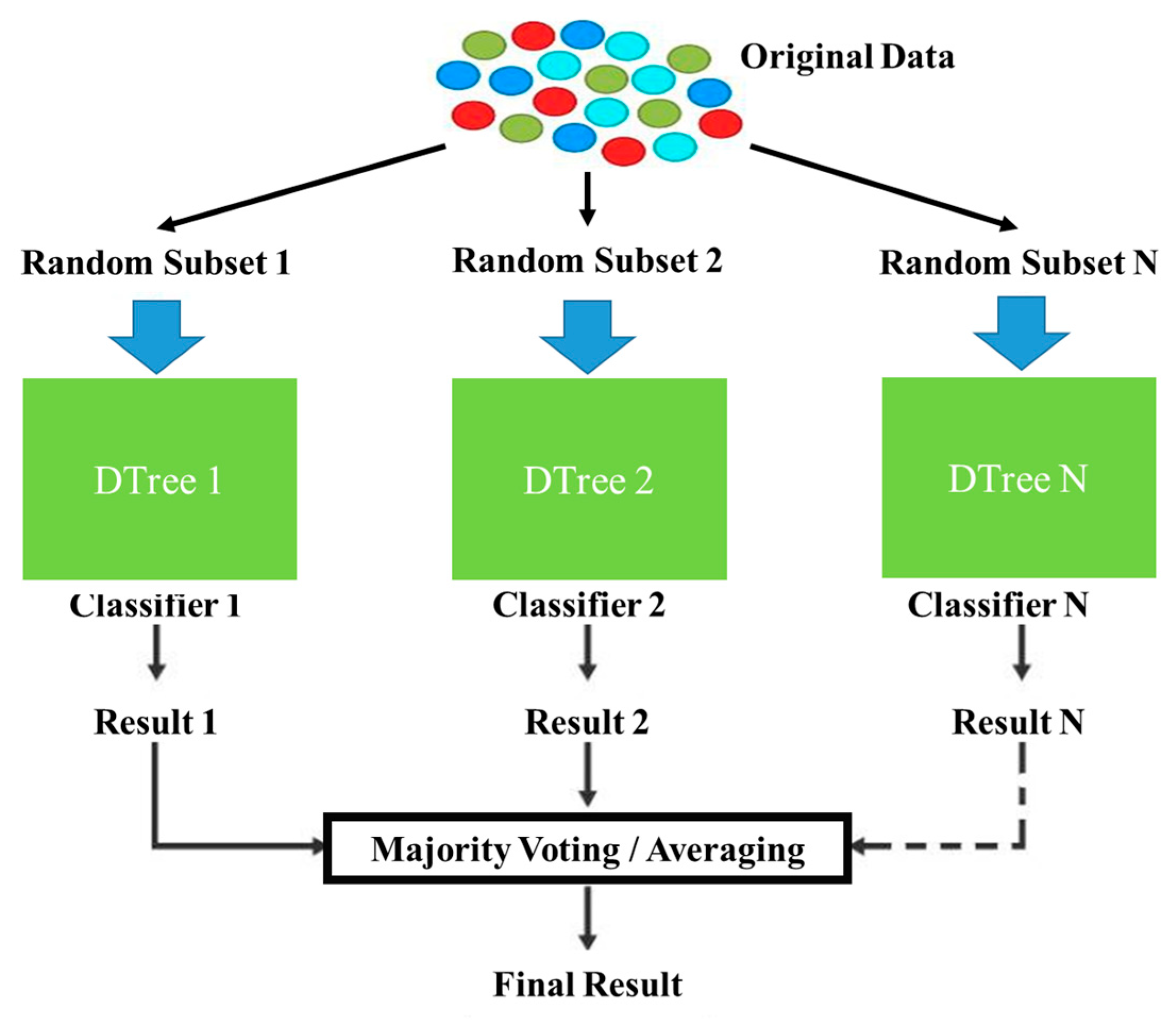
• Adoption of the Ensemble Learning classification algorithm to build a noise-resilient and stable model capable of accurately detecting various types of malware, ultimately enhancing the overall performance and robustness of the proposed approach.

The general architecture of the article is as follows: relevant studies are described in Section 2 and a suggested method is presented in Section 3. In the Section 4, the simulation and analysis of the simulation results are explained. Finally, Section 5 concludes the study.

2. Related Works

Numerous studies have focused on malware classification for both Microsoft Windows and Android platforms [17,18,19,20,21]. However, despite these dedicated efforts, effective malware classification across both environments faces inherent and persistent challenges. These challenges primarily stem from the continuous evolution, increasing sophistication, and highly differentiated nature of modern malware variants, regardless of their target operating system [22,23]. Consequently, and particularly in light of the continuously growing number of newly emerging and highly differentiated malware, the robust classification of both Android and Windows malware families has emerged as a critical area of research for many scholars and professionals [24]. So, numerous diverse methods have been proposed for the classification of these malware types, some of which are reviewed in the following.

Another issue associated with the classification of malware using machine learning techniques is that the behavior of these programs is constantly changing [25,26,27]. A number of researchers have dealt with this problem with the help of model aging or degradation and have suggested solutions [28,29]. For instance, the DroidSpan classifier [28] performs better than five benchmark detectors that were used in the analysis for sustainability by utilizing a behavioral profiling method on applications. In a similar vein, DroidEvolver [29] proposed an adaptive model update method which is developed using the pool of linear online learning and delayed classifiers to keep the performance consistent in the long run.

In [30], the authors propose a Hierarchical Convolutional Network (HCN) for the classification of malware. HCN was designed to contain two levels of convolutional layers within the mnemonic and function levels to extract n-gram-like features and improve classification results. A comparative analysis showed that the proposed method yielded better results than the previous models based on deep learning. However, the reliance on n-gram-like features extracted from specific levels might limit its ability to generalize to heavily obfuscated or entirely novel malware samples that do not exhibit similar patterns. Another study [31] proposed a malware detection approach using a one-dimensional convolutional neural network (1D-CNN). This method takes binary files as inputs and applies the 1D convolution in order to extract features. There is also a preview stage involved in the proposed system, and the system was validated using an F-IDF-based malware detector that had better precision as well as speed in comparison with other approaches. A potential limitation of this approach is its dependence on raw binary features, which can be highly sensitive to minor changes in the malware structure, potentially hindering its effectiveness against polymorphic variants.

In [32], the authors proposed a Windows malware detection system that uses CNN features of Portable Executable (PE) files. A 10-fold cross-validation was conducted, resulting in detection with an accuracy of 97.96%, allowing existing methods to be overcome in terms of accuracy and time. Despite high accuracy, this method might struggle with non-PE file malware or those specifically designed to evade PE file analysis, as its feature extraction is solely based on PE file characteristics.

In [33], the authors follow a similar concept but with a mix of both methods, where PE files are converted to color images and then features are extracted using a tuned deep learning framework. These features are then analyzed using a Support Vector Machine (SVM) to classify them into different categories. This helps in avoiding the feature engineering task as deep learning and machine learning methods are combined, which results in a better detector. While combining deep learning and machine learning can be effective, the conversion of PE files to color images might introduce an information loss or create vulnerabilities to adversarial attacks specifically designed to manipulate image representations.

In [34], the authors proposed a deep learning-based hybrid architecture for the classification of different types of malware. The system put forward here is based on two deep neural network models trained on different corpora and it has four principal steps: the acquisition of data, establishing the network, training, and assessment. The usefulness of the provided approach is illustrated with respect to benchmarks like Malimg, Microsoft BIG 2015, and Malevis. The reliance on specific, potentially static, benchmark datasets might limit its real-world applicability, as malware evolution can quickly render models trained on outdated datasets less effective.

More recent work that has been proposed in [35] is the API-MalDetect software that provided an API call-based malware detection approach using deep learning. The encoding of API call sequences is fulfilled with a natural language processing (NLP)-based encoder and a feature extractor consisting of the CNN and Bidirectional Gated Recurrent Units (BiGRU). It is developed in a way that it can detect new types of malware and enhance its functionality when there is a change in the rate of exposed malware by eliminating temporal and spatial repetition between training and testing. Although designed for new malware detection, this approach’s effectiveness is heavily dependent on the completeness and diversity of the API call sequences it processes, and it might be bypassed by malware employing sophisticated API obfuscation techniques or non-API-based malicious activities.

In [36], a new architecture for malware detection named LGMal was introduced based on both local and global features. Proposed to tackle the cybersecurity issues of smart cities, this approach is focused on combining cumulative CNNs with GCNs. The CNN module extracts sequence features from the API call sequences which represent the local semantic of the programs while the GCN module captures the structure of the semantic API graph meaning that the model captures both local and global features for the effective detection of the malicious software. While capturing both local and global features is promising, the complexity of combining CNNs and GCNs could lead to high computational costs and require extensive training data, potentially limiting its scalability in resource-constrained environments.

3. Materials and Methods

In this paper, an efficient method for malware detection is proposed based on a novel deep neural network called Hybrid ResNet-Transformer (HRT-Net) and a Wrapper-based feature selection method using the Improved Grasshopper Optimization Algorithm (IGOA). In the first stage, features are extracted from malware images using the deep neural network HRT-Net. Due to its powerful architecture, this network is capable of extracting complex and high-level features from image data. In the proposed network, local features are captured by the convolutional layers of the ResNet architecture, while global features are extracted using Transformer layers. The ResNet component, by leveraging residual connections and deep convolutional layers, can effectively identify local patterns such as edges, textures, and fine-grained details in malware images. On the other hand, the Transformer component utilizes a multi-head attention mechanism to understand long-range dependencies and complex relationships within the image, thereby extracting higher-level patterns and semantic associations. Ultimately, the extracted local and global features are concatenated to form a comprehensive and rich representation of the malware image, capable of accurately detecting complex patterns and unknown threats. This comprehensive feature representation is then passed to the Improved Grasshopper Optimization Algorithm (IGOA) with dynamic inertial motion weights and dynamic mutation coefficient, where less significant features are discarded, and only the most relevant features for malware detection are retained. Finally, the optimized set of features is fed into an Ensemble Learning classifier, which performs malware detection with high accuracy and robustness. The diagram of the proposed method is illustrated in Figure 1.

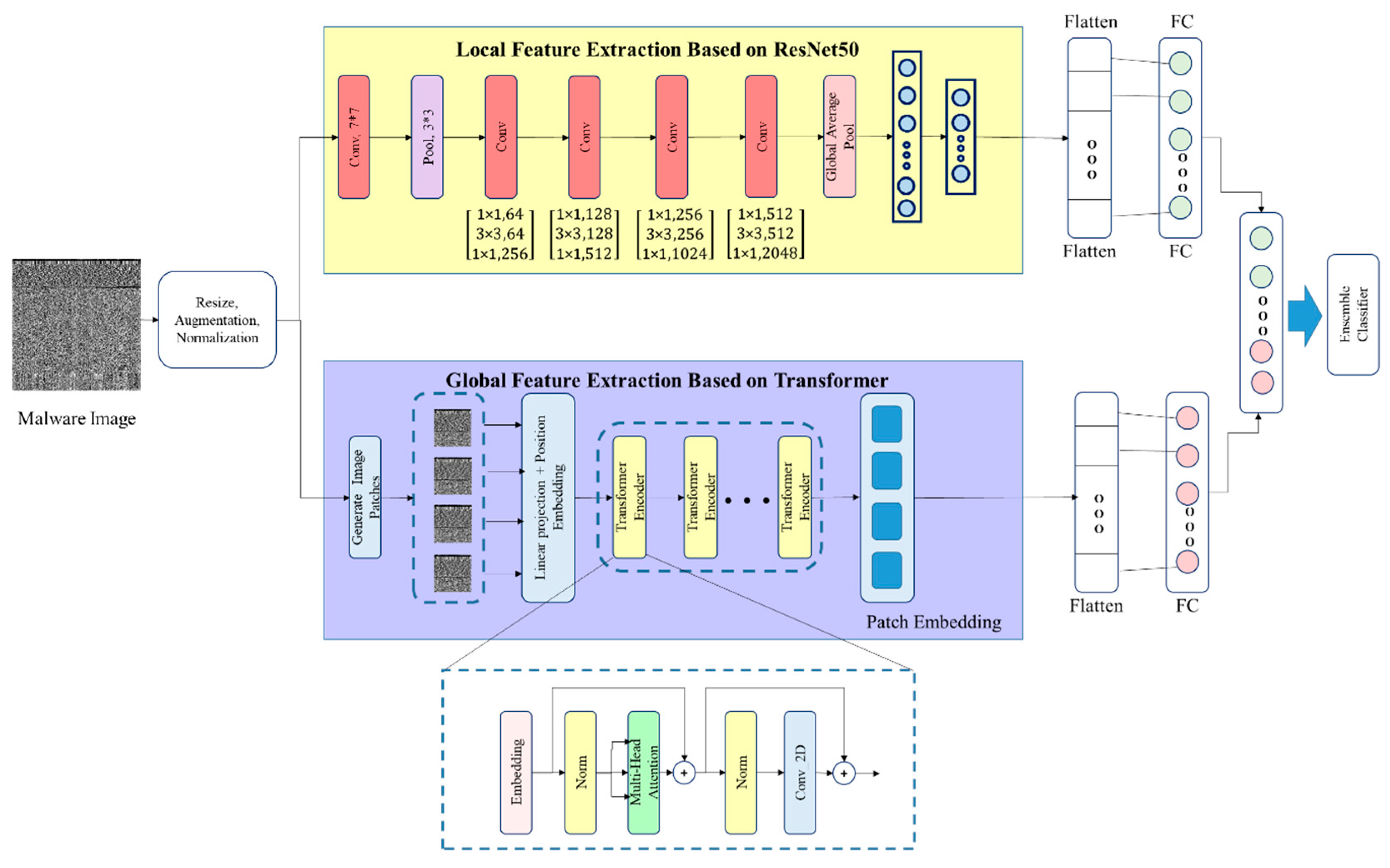
3.1. Feature Extraction Using Hybrid Resnet-Transformer Network (HRT-Net)

The proposed hybrid deep neural network (HRT-Net) is employed to extract both local and global features from malware images. The aim of utilizing this architecture is to achieve a deep, rich, and multi-perspective representation of the malware image data, allowing for the accurate modeling of their complex and multidimensional patterns. HRT-Net integrates two distinct branches: one based on the ResNet50 convolutional neural network for local feature extraction, and another based on the Transformer architecture for capturing global dependencies. By leveraging the complementary strengths of these two architectures, the network is capable of simultaneously extracting fine-grained spatial details (such as edges, textures, and localized patterns) and high-level global representations (such as semantic relationships and long-range dependencies).

The first branch of the network employs ResNet50 to extract local features [37]. The initial layer in this path applies a convolution operation with a 7 × 7 kernel and a stride of 2, which serves to capture low-level structures such as edges and texture primitives. This is followed by a 3 × 3 max pooling layer with a stride of 2, used to reduce the spatial dimensions and improve the model’s robustness to local variations. Subsequently, the image passes through four residual blocks, each composed of three convolutional layers with kernel sizes 1 × 1, 3 × 3, and 1 × 1, respectively. The first layer reduces the channel dimensions, the second captures complex local features, and the third restores the channel depth. These blocks incorporate shortcut connections to mitigate the vanishing gradient problem and facilitate training in deep networks. The mathematical formulation of the residual connection is as follows:

$$y=\mathcal{F}\left(x·\left\{w_i\right\}\right)+x$$

(1)

where $\mathcal{F}$ represents the transformation learned by the convolutional layers and $x$ is the input to the residual block. At the end of the ResNet path, a global average pooling layer aggregates spatial information by computing the mean over the entire feature map, producing a compact and translation-invariant feature vector. This vector is then flattened and passed through a fully connected (FC) layer to form the final local feature representation.

The second branch utilizes a Transformer-based architecture to extract global features and capture long-range dependencies. Initially, the image is divided into a sequence of non-overlapping patches. Each patch is linearly projected into a fixed-dimensional embedding vector. To preserve spatial information, positional encodings are added to these embeddings. The resulting sequence is then fed into a stack of Transformer encoder blocks, each comprising the following components:

• Layer Normalization: Stabilizes and accelerates training by normalizing the input features.
• Multi-Head Self-Attention: Enables the model to learn dependencies between distant regions of the image. This mechanism uses query (Q), key (K), and value (V) matrices to compute attention scores, defined as follows:

  $$Attention\left(Q·K·V\right)=softmax\left({\displaystyle \frac{Q{K}^T}{\sqrt{d_k}}}\right)V$$

  (2)

  where $d_k$ is the dimensionality of the key vectors, and the softmax function normalizes the attention weights.
• Two-layer Feedforward Network (MLP): Enhances the model’s nonlinearity and capacity to learn higher-order feature interactions.

To further enhance spatial modeling, a 2D convolutional layer is added after each Transformer block. This layer helps capture spatial dependencies that may not be fully modeled by the attention mechanism alone. The output of the Transformer path is also flattened and passed through a fully connected layer to yield the final global feature representation.

Finally, the local and global feature vectors from the ResNet50 and Transformer branches are concatenated to form a unified, comprehensive feature representation. This fusion integrates fine-grained spatial details and high-level semantic structures into a shared feature space, enabling robust and accurate malware pattern recognition. The HRT-Net architecture, through this dual-branch design, provides a novel and effective approach for feature extraction in malware classification tasks, representing the core innovation of this study. Figure 2 illustrates the architecture of the proposed hybrid deep neural network, HRT-Net, designed for feature extraction.

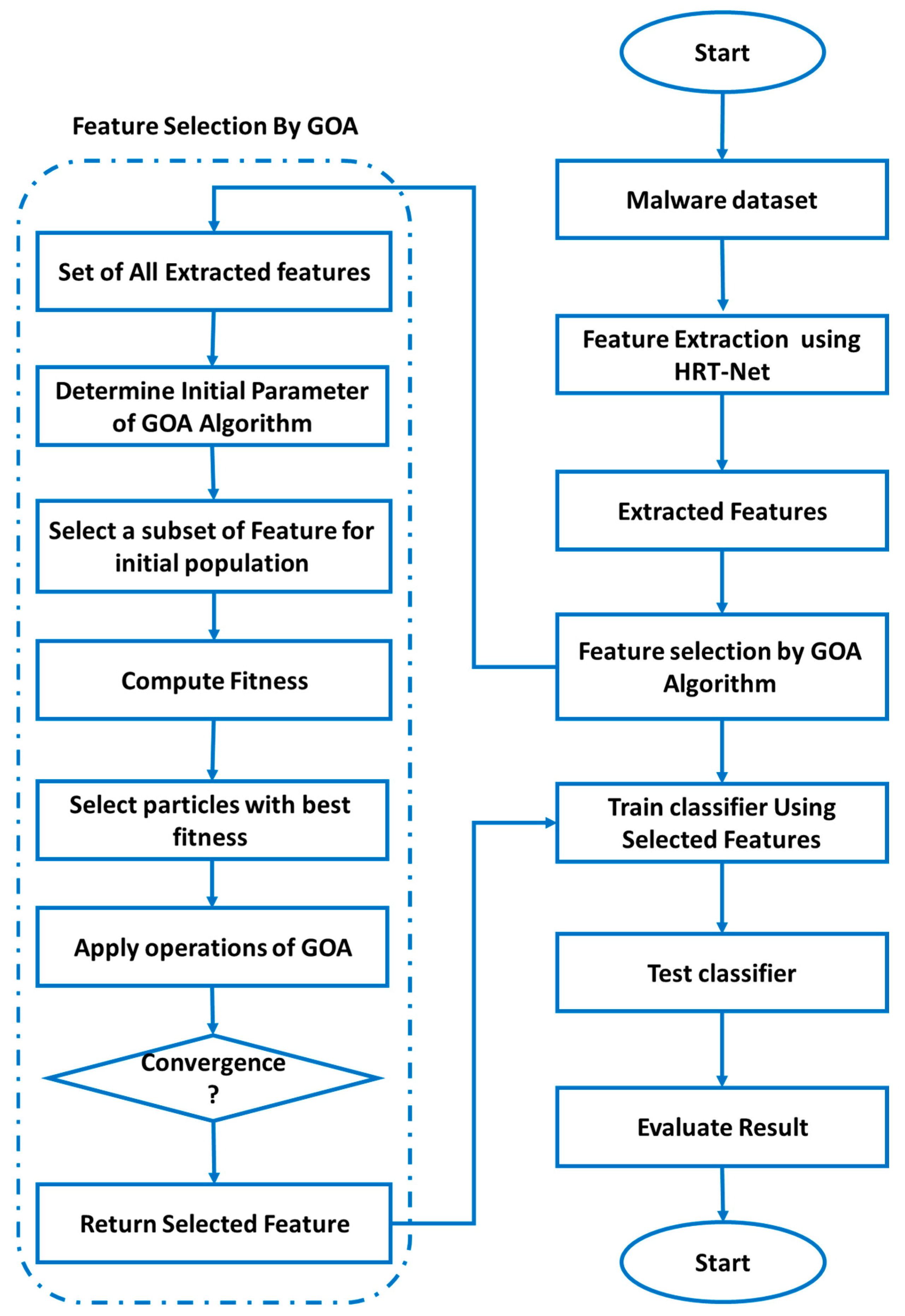
3.2. Selection of Optimal Features with the Improved Grasshopper Optimization Algorithm

In this study, an Improved Grasshopper Optimization Algorithm (IGOA) is employed to select an optimal subset of features. The selection of optimal features reduces unnecessary dependencies among features, thereby enabling the classification model to focus on more informative and discriminative attributes. This, in turn, leads to improved detection accuracy and reduced error rates. The standard Grasshopper Optimization Algorithm (GOA), inspired by the social interactions among grasshoppers through information sharing and cooperative behavior, demonstrates strong capabilities in exploring the search space and identifying optimal solutions. These interactions enable grasshoppers to effectively converge toward optimal regions while avoiding entrapment in local optima. As a result, GOA can accurately identify the most relevant features and enhance the performance of malware detection models.

In this work, the improved version of the GOA is utilized for feature selection, wherein the optimization capability of the algorithm is enhanced by incorporating a dynamic mutation factor and adaptive inertial motion weights. These modifications improve the algorithm’s convergence behavior and overall performance in locating optimal feature subsets. The process of applying the IGOA for optimal feature selection is outlined as follows:

• Step 1: Initialization of Parameters

In this step, the key algorithmic parameters—such as the number of grasshoppers, the maximum number of iterations, and other configuration settings—are initialized. These parameters play a critical role in influencing the convergence speed and the overall performance of the algorithm.

• Step 2: Generation of Initial Population

An initial population of grasshoppers is randomly generated within the problem’s search space. Each grasshopper represents a potential solution, corresponding to a candidate subset of selected features. The position of each grasshopper encodes a feature subset that may represent an optimal selection. During the optimization process, the positions of grasshoppers are iteratively updated to guide the population toward optimal feature sets.

• Step 3: Evaluation of the Fitness Function

To assess the quality of each solution, a fitness function is defined. In this study, malware detection accuracy is employed as the fitness criterion. The feature subsets selected by IGOA are fed into an Ensemble Learning model, and the model’s classification accuracy is computed as the fitness value for each grasshopper. A higher accuracy score indicates a more effective feature subset and, consequently, a better solution in the context of the optimization process.

$$fitness=Accuracy={\displaystyle \frac{TP+TN}{TP+TN+FP+FN}}$$

(3)

In the above equation, the symbols TP, TN, FP, and FN, respectively, represent the number of True Positives (correct identification of positive samples), True Negatives (correct identification of negative samples), False Positives (incorrect classification of negative samples as positive), and False Negatives (incorrect classification of positive samples as negative).

• Step 4: Identification of the Best Discovered Solution $\widehat{{\mathit{T}}_{\mathit{d}}}\mathsf{\left(}\mathit{t}\mathsf{\right)}$

In this step of the Improved Grasshopper Optimization Algorithm, the solution with the highest fitness value within the current population is identified as the best solution in the current iteration. This solution is then compared to the best solutions obtained in the previous iterations. If it exhibits superior performance, it replaces the previous best and is stored as the global best solution discovered thus far.

• Step 5: Position Update of Grasshoppers

In this step, the position of each grasshopper is updated based on the position update mechanism defined in the IGOA structure. This update is performed using the following equation, with the aim of steering the grasshoppers toward the optimal region in the search space:

$$X_i=S_i+G_i+A_i$$

(4)

The variable $S_i$ in the above equation represents the social interaction among grasshoppers and is calculated using Equation (5).

$$S_i=\sum _{j=1(j\ne i)}^{nPop}s\left(d_{ij}\right){\widehat{d}}_{ij}$$

(5)

In the above equation, the distance between the i-th and j-th grasshoppers is denoted by $d_{ij}$. Additionally, the unit vector between the i-th and j-th grasshoppers is represented by ${\widehat{d}}_{ij}$. The strength of the social interactions is modeled by the function s.

Furthermore, the variable G_i in Equation (4) represents the gravitational force of the i-th grasshopper, which is determined by Equation (6).

$$G_i=-g{e}_g$$

(6)

In Equation (4), the gravitational force of the Earth is denoted by g, and the unit vector pointing toward the center of the Earth is represented by e_g.

Additionally, the variable A_i in Equation (4) represents the wind flow for the i-th grasshopper, which is determined by Equation (7).

$$A_i=-u{e}_w$$

(7)

In the equation above, the variable u represents the constant thrust, and e_w is the unit vector in the direction of the wind.

Considering the above equations, the motion equation for the grasshoppers is rewritten as follows:

$$X_i=\sum _{j=1(j\ne i)}^{nPop}s\left(\left|x\left(i\right)-x\left(j\right)\right|\right){\displaystyle \frac{x\left(i\right)-x\left(j\right)}{d_{ij}}}-g{e}_g-u{e}_w$$

(8)

However, the initial mathematical model proposed for the Grasshopper Optimization Algorithm may not be directly applicable for solving real-world optimization problems. The primary reason for this limitation is that grasshoppers quickly converge to a region known as the “comfort zone,” but this convergence does not necessarily lead to a specific point in the search space. As a result, the clustering of grasshoppers in a fixed region prevents the algorithm from reaching the global optimal point. To overcome this challenge, a modified version of the position update equation for the grasshoppers has been introduced. This modification is designed to enhance convergence accuracy and improve search efficiency, especially in complex optimization problems.

$$x_i^d\left(t+1\right)=c_{IGOA}\left\{\sum _{j=1(j\ne i)}^{nPop}{c}_{D\_GOA}{\displaystyle \frac{{ub}_d-{lb}_d}{2}}s\left(\left|x\left(i\right)-x\left(j\right)\right|\right){\displaystyle \frac{x\left(i\right)-x\left(j\right)}{d_{ij}}}\right\}+{\widehat{T}}_d(t)$$

(9)

In Equation (9), the next position of the i-th grasshopper is denoted as X_i^d(t + 1), the positions of all other grasshoppers are denoted as x_j(t), and the current position of the i-th grasshopper is represented as xi(t)x_i(t)xi(t). The dynamic inertia weight, which maintains the balance between exploration and exploitation and reduces the attraction, neutral, and repulsion zones as the number of algorithm iterations increases, is represented by $c_{IGOA}$. Additionally, in this equation, the target position is represented by $\widehat{T_d}\left(t\right)$.

• Step 6: Update of Dynamic Inertia Weight

Since in the Grasshopper Optimization Algorithm (GOA) the position update of the grasshoppers is carried out only around the best global position, the algorithm faces two main challenges: becoming trapped in local optima and having a low convergence rate during the search process. To overcome these limitations, this study introduces the concept of dynamic inertia weight within the framework of the Improved Grasshopper Optimization Algorithm (IGOA). This mechanism is designed to enhance the convergence speed and improve the balance between the exploration and exploitation processes.

Inertia weight directly controls the speed of the particles at each stage of the optimization process and determines how much a particle tends to maintain its previous motion trajectory. High inertia weight values cause particles to maintain their previous momentum, allowing them to explore farther distances in the search space. As a result, the ability to explore the problem space is enhanced. On the other hand, smaller inertia weights reduce the range of motion of the particles and cause them to focus more on the local areas around the best current solution, which improves exploitation and search accuracy.

Based on these characteristics, it can be concluded that larger inertia weights are more suitable for improving the exploration process, while smaller weights are more appropriate for enhancing local exploitation. Therefore, in the proposed structure of the IGOA, the inertia weights are dynamically and adaptively adjusted, and their values decrease nonlinearly and exponentially as the number of iterations increases. This adaptive adjustment improves the performance of the algorithm in searching the solution space and accelerates its convergence speed.

As a result, in Step 6 of the IGOA execution process, the parameter is updated using Equation (10) to effectively apply the inertia weighting mechanism.

$$c_{IGOA}=b\times c_{min}{\left({\displaystyle \frac{c_{min}}{c_{max}}}\right)}^{{\displaystyle \frac{1}{\left(\frac{1+t}{t_{max}}\right)}}}$$

(10)

In Equation (10), the maximum value of $c_{IGOA}$ (which is typically close to 1) is represented by c_max, and the minimum value of $c_{IGOA}$ (which is typically close to 0 and positive) is denoted by c_min. Additionally, in this equation, b is a random number around the value of 1, t is the current iteration, and t_max is the maximum number of iterations.

• Step 7: Application of Jumping Based on Dynamic Jump Probability Coefficient and Triangular Jump Strategy

To enhance the performance of the Improved Grasshopper Optimization Algorithm (IGOA), a dynamic jumping probability coefficient has been introduced. The value of this coefficient gradually increases as the number of iterations increases. The purpose of using this coefficient is to increase the probability of a more effective exploration of the search space by the grasshoppers, thus improving the algorithm’s ability to escape local optima.

The gradual increase in this coefficient expands the search range in the later stages of the algorithm, enabling the discovery of unknown regions and leading to better solutions. In other words, this mechanism plays an effective role in improving the algorithm’s adaptive exploration. The dynamic jumping probability coefficient is calculated based on Equation (11), which will be explained below.

$$p_m=0.2+0.5\times {\displaystyle \frac{t}{T}}$$

(11)

In the proposed version of the Improved Grasshopper Optimization Algorithm (IGOA), a triangular jump strategy is employed to implement the jump operator. The use of this strategy increases the diversity of the population, thereby reducing the likelihood of the algorithm becoming trapped in local optima during the search process.

In this method, three grasshoppers are first selected randomly from the population. Then, their position information is combined using Equation (12), and a new position resulting from the jump is generated. This approach results in the creation of more diverse and efficient solutions in the search space.

$$X\left(t\right)={\displaystyle \frac{X_{rg1}+X_{rg2}+X_{rg3}}{3}}+(p2-p1)\times (X_{rg1}-X_{r2})+(p3-p2)\times (X_{rg2}-X_{rg3})+(p1-p3)\times (X_{rg3}-X_{rg1})$$

(12)

In the above equation, the variables $X_{rg1}$, $X_{rg2}$, and $X_{rg3}$ represent the grasshoppers that are randomly selected. Additionally, the variables $p1$, $p2$, and $p3$ are the weights of the disturbed components, which are calculated using Equation (13).

$$p1={\displaystyle \frac{\left|f\left(X_{rg1}\right)\right|}{\acute{p}}}$$

(13)

$$p2={\displaystyle \frac{\left|f\left(X_{rg2}\right)\right|}{\acute{p}}}$$

(14)

$$p3={\displaystyle \frac{\left|f\left(X_{rg3}\right)\right|}{\acute{p}}}$$

(15)

In Equations (13)–(15), the constant $\acute{p}$ is calculated using Equation (16). Additionally, in these relations, f(.) represents the fitness function.

$$\acute{p}=\left|f\left(X_{r1}\right)\right|+\left|f\left(X_{r2}\right)\right|+\left|f\left(X_{r3}\right)\right|$$

(16)

The use of the triangular jump strategy ensures that the combination of the positions of three randomly selected grasshoppers provides the algorithm with more diverse information about the search space, rather than relying solely on the nearest position to the local optimum. This approach prevents the update of the grasshoppers’ positions based purely on solutions in the vicinity of the best local position, thereby effectively reducing the likelihood of the algorithm becoming trapped in local optima. The increased diversity in generating new positions is one of the key factors in improving the overall performance of metaheuristic algorithms.

• Step 8: Stopping Condition

Steps 3 to 7 of the algorithm are executed repeatedly until the stopping condition is met. In the proposed method, the stopping condition is defined as reaching the predefined maximum number of iterations. Afterward, the best solution obtained throughout the execution process is reported as the final output of the algorithm.

3.3. Classification Using Ensemble Learning Technique

The proposed model employs an Ensemble Learning approach, where the decision-making process is based on the combination of results from multiple distinct classifiers. In this work, the data is divided into several subsets, each processed by a different classifier. Specifically, a decision tree classifier is used as the base classifier. This choice enables the model to capture different patterns and features within the data, thus improving the overall classification performance. To further enhance the accuracy of the classification process, overlapping portions of data are used across the classifiers. In other words, some data segments are fed into multiple classifiers, increasing the likelihood of correctly classifying difficult or ambiguous instances. This approach provides the classifiers with additional opportunities to refine their decisions, ultimately improving classification accuracy. The ensemble approach offers significant advantages when dealing with noisy data or class imbalance, where individual classifiers may struggle. By combining the predictions of various classifiers, the model mitigates the weaknesses of each individual method, resulting in a more accurate and reliable classification process. This method also reduces the risk of local optima entrapment, enhancing the model’s ability to generalize to new, unseen data [38]. As illustrated in Figure 3, this Ensemble Learning approach incorporates methods such as Bagging, Majority Voting, and data partitioning. Bagging, or Bootstrap Aggregating, involves creating multiple subsets of the training data by sampling with replacement, which allows the model to train multiple classifiers on different data subsets. The predictions from each classifier are then aggregated to form a final decision. This reduces variance and helps improve the model’s robustness, especially in cases where the data is noisy or contains outliers. Majority Voting, another key operation in the ensemble method, is employed to combine the predictions of all individual classifiers. Each classifier votes for a class, and the final prediction is based on the majority vote. This strategy ensures that the model’s decision is influenced by the collective strength of all classifiers, further enhancing accuracy and reducing the likelihood of misclassification. These techniques, as depicted in Figure 3, work together to improve the model’s overall performance. The combination of Bagging and Majority Voting not only increases the model’s accuracy but also strengthens its ability to detect complex patterns in malware data, providing a more reliable and scalable solution for malware detection.

3.4. Investigating the Feature Selection Process on Computational Complexity in the Classification Stage

The computational complexity of Ensemble Learning classifiers, particularly using the Bagging method, is a key factor in evaluating model efficiency. It directly depends on the number of learners (M), the number of training data samples ($K_{train}$), and the dimensionality of features (where the total number of features is $N_{tot}$). In the classification scenario with the full set of $N_{tot}$ features for each instance, the training phase of the ensemble classifier (using decision trees as base learners) has a computational complexity of $O(M·K_{train}·N_{tot}·\mathrm{l}\mathrm{o}\mathrm{g}(K_{train}\left)\right)$, while the prediction phase for $K_{test}$ test samples exhibits a complexity of $O(K_{test}·M·N_{tot})$. However, when the optimal feature selection process is applied and the data dimensionality is reduced from $N_{tot}$ to $N_s$ (where $N_s$ is the number of selected features), the computational complexity significantly decreases in both phases. More precisely, the training phase complexity in this case is reduced to $O(M·K_{train}·N_s·\mathrm{l}\mathrm{o}\mathrm{g}(K_{train}\left)\right)$, and the prediction phase complexity to $O(K_{test}·M·N_s)$. This dimensionality reduction implies a direct decrease in computational complexity proportional to $N_{tot}/N_s$, which not only optimizes training and prediction times but also significantly contributes to improving computational resource consumption and overall model efficiency in real-world applications. Overall, despite the feature selection process itself potentially having its own computational overhead (typically performed once and offline), the substantial reduction in complexity during the training and, especially, the prediction phases of the final model, offer a significant advantage in the implementation and deployment of Ensemble Learning-based classification systems.

4. Results

In this section, our goal is to evaluate and compare the outcomes attained by the simulation of the presented approach. The software used in this work to simulate the suggested method is MATLAB 2024. In this section, the evaluation criteria of the suggested technique are presented along with the description of the database used, as well as the analysis of the results obtained from the simulation.

4.1. Database

In this work, the Malimg dataset available on the Kaggle website [39] was used. The Malimg dataset is a benchmark for classifying malware that is available to the public on Kaggle. The database comprises 9435 executable files of malware spanning 25 distinct malware categories. The malware files have been converted into 32 × 32 images using nearest neighbor interpolation. This dataset contains various types of malware that are shown in

Table 1. Malimg dataset contents.

#	Class	Family	#	Class	Family
1	Worm	Allaple L	14	Trojan	Alueron.gen!J
2	Worm	Allaple A	15	Trojan	Malex.gen!J
3	Worm	Yuner A	16	PWS	Lolyda AT
4	PWS	Lolyda AA 1	17	Dialer	Adialer.C
5	PWS	Lolyda AA 2	18	TDownloader	Wintrim BX
6	PWS	Lolyda AA 3	19	Dialer	Dialplatform B
7	Trojan	C2Lop.P	20	TDownloader	Dontovo A
8	Trojan	C2Lop.gen!g	21	TDownloader	Obfuscator.AD
9	Dialer	Instantaccess	22	Backdoor	Agent. FYI
10	TDownloader	Swizzot.gen!I	23	Worm AutoIT	Autorun K
11	TDownloader	Swizzor.gen!E	24	Backdoor	Rbot!gen
12	Worm	VB.AT	25	Trojan	Skintrim N
13	Rogue	Fakerean

.

For instance, three types of malware class are illustrated in Figure 4.

4.2. Evaluation Metric

To study the improvement of the proposed system, there are statistical parameters that can be studied (Accuracy, Precision, Recall, and F1). The accuracy is as described by Equation (17):

$$Accuracy={\displaystyle \frac{(TruePositive+TrueNegative)}{\left(TruePositive+FalsePositive+TrueNegative+FalseNegative\right)}}$$

(17)

Precision (P) is calculated to discover the number of relevant instances among the total instances. And it written by Equation (18):

$$Precision={\displaystyle \frac{TruePositive}{TruePositive+FalsePositive }}$$

(18)

Recall (R) is an indicator of the ratio of correct relevant instances to the relevant instances in the whole test. Recall is calculated as shown in Equation (19):

$$Recall={\displaystyle \frac{TruePositive}{TruePositive+FalseNegative}}$$

(19)

Finally, the F1-score is a connection between Precision and Recall, resulting Equation (20):

$$F_{1}score={\displaystyle \frac{2\times Percision\times Recall}{(Percision+Recal)}}$$

(20)

In Equations (17)–(20), the terms True Positive (TP), False Positive (FP), False Negative (FN), and True Negative (TN) are used to represent different types of detections:

• True Positive (TP): Refers to the samples that are truly identified as positive.
• False Positive (FP): Indicates the samples that are falsely identified as positive.
• False Negative (FN): Represents the samples that are wrongly identified as negative.
• True Negative (TN): Refers to the samples that are correctly identified as negative.

4.3. Results Evaluation

In this section, an analysis of the presented approach performance in comparison with other methods, a simulation of the presented approach, and the comparison of the experiment outcomes are described. The results of Precision, Accuracy, Recall, and F1-score criteria are shown in several figures and tables. For the experiments to be carried out, the database was split into two sets: training and test. The training phase is controlled by the training set. During the training of the neural network, these data are used to modify the weights of the network. These data are used alone to determine the accuracy and how well the network can perform in the new scenarios of the trained network. In the learning process, 70% of the dataset is used for training the system while the remaining 30% is used for testing purposes in the experiments; 10-fold cross-validation is used to assess the performance of the system. In the first experiment the indicators for the evaluation of the presented method are shown.

4.3.1. Evaluation of Training Process for Ensemble Learning

In this section, the effectiveness of the Ensemble Learning algorithm in the detection process is analyzed by way of its learning curves. Figure 5 displays two subplots illustrating the convergence behavior of the Ensemble Learning algorithm in terms of both accuracy and loss, evaluated on both training and validation datasets. In both subplots, the horizontal axis represents the number of base learners. The upper subplot’s vertical axis represents the accuracy of the model, while the lower subplot’s vertical axis represents the loss. Evaluating these curves is crucial for understanding the efficiency of the proposed approach and the influence of increasing the number of learners on the model’s performance. In the beginning, that is, when there are relatively few learners, the accuracy and loss curves exhibit noticeable oscillations. This is because the ensemble models are highly dependent on the individual base learners and have not yet fully learned generalization at this early stage. As the number of learners increases, to around 5 to 10 learners, both the training and validation accuracy rapidly converge to an optimal level of nearly 1.0 (or 100%). Concurrently, the training and validation loss dramatically decrease and stabilize at very low values, indicating a significant reduction in prediction error. This simultaneous convergence of both accuracy and loss for both datasets highlights the robustness and stability of the ensemble model. This trend shows that the Ensemble Learning method does indeed have the ability to improve the performance of the model by integrating the results of diverse learners. Thus, after a certain number of learners (approximately 5 to 10), the model convergence stabilizes, and both accuracy and loss remain nearly constant, with minimal differences between training and validation performance. This consistent behavior across both datasets suggests that the model generalizes well and does not significantly overfit. Specifically, the convergence behavior observed in both the accuracy and loss curves indicates that the proposed Ensemble Learning approach is effective and efficient for the detection of malware. It demonstrates that the algorithm achieves a high level of accuracy with a small number of learners, and further increasing the number of learners beyond this point results in only a marginal improvement in accuracy and a minimal reduction in loss. This clearly illustrates how Ensemble Learning enhances the accuracy levels and minimizes the prediction error rates by efficiently combining the strengths of multiple base learners. Moreover, the rapid rate of convergence of the model, as seen in both the accuracy increase and loss decrease, shows that the combination of various models in an ensemble helps the malware detection model to learn better and become less sensitive to noise, leading to stable and high performance on unseen data. However, based on the observations made from the results obtained, the proposed method can be seen as a potential solution for cybersecurity use, especially in cases of detecting new or emerging malware threats.

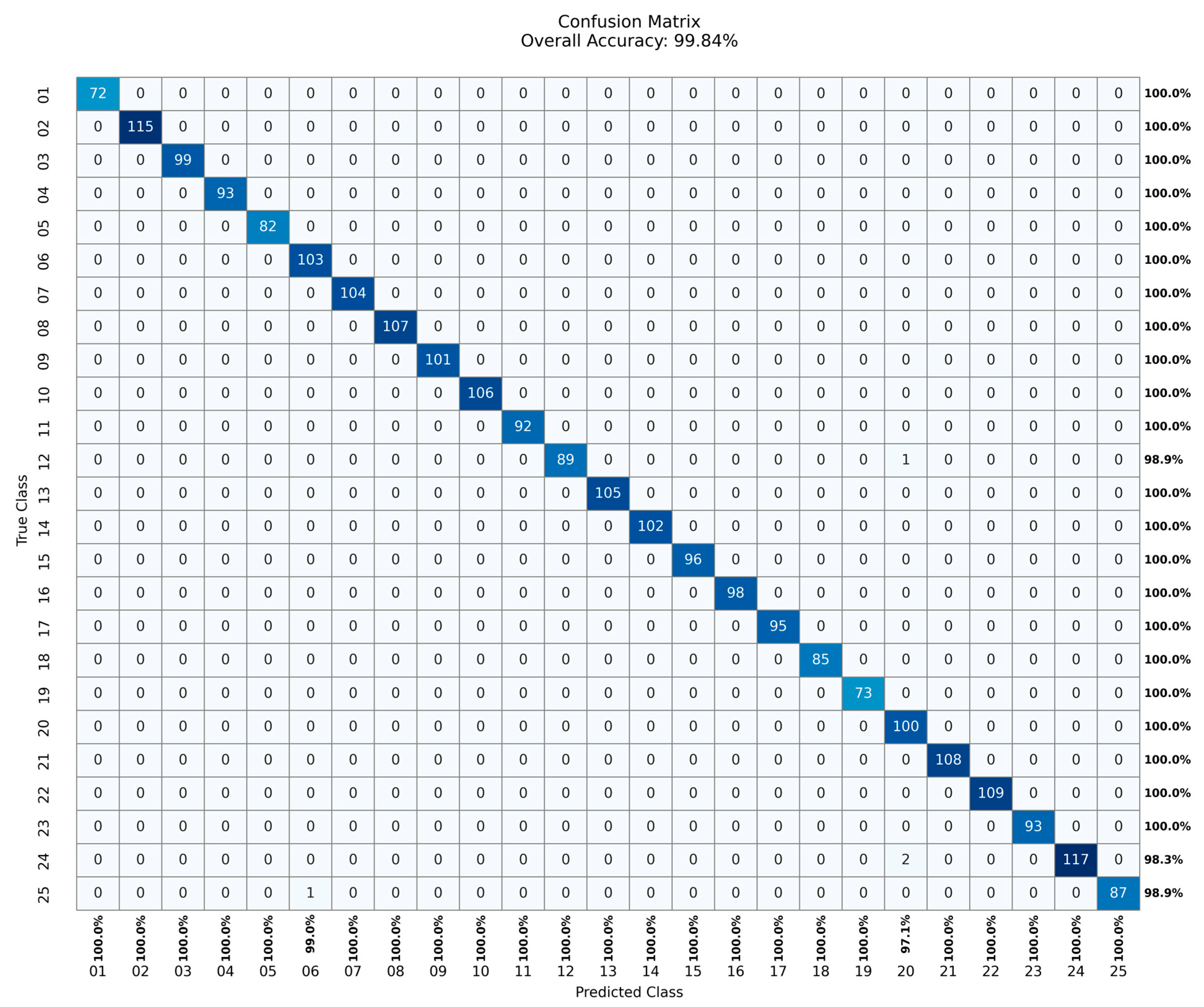
4.3.2. Evaluation of Test Process for Ensemble Learning

The confusion matrix of the malware classification is shown in Figure 6 below. The confusion matrix helps to determine the performance of the classifier for each class of data. The accuracy of each class is written down on the right side of the matrix, in the column corresponding to this class. From the results presented in Figure 5, it can be observed that there was a perfect classification for all the classes with the exception of 12, 24, and 25. For these classes the classification accuracy was established to be 98.9%, 98.3%, and 98.9%, respectively. The results reflect the proper efficiency of the presented approach to malware classification. As can be seen, this matrix is made for one execution, and the results are slightly different for each of the executions. To make the comparison with other methods possible, the results have been computed as an average of 50 programs running.

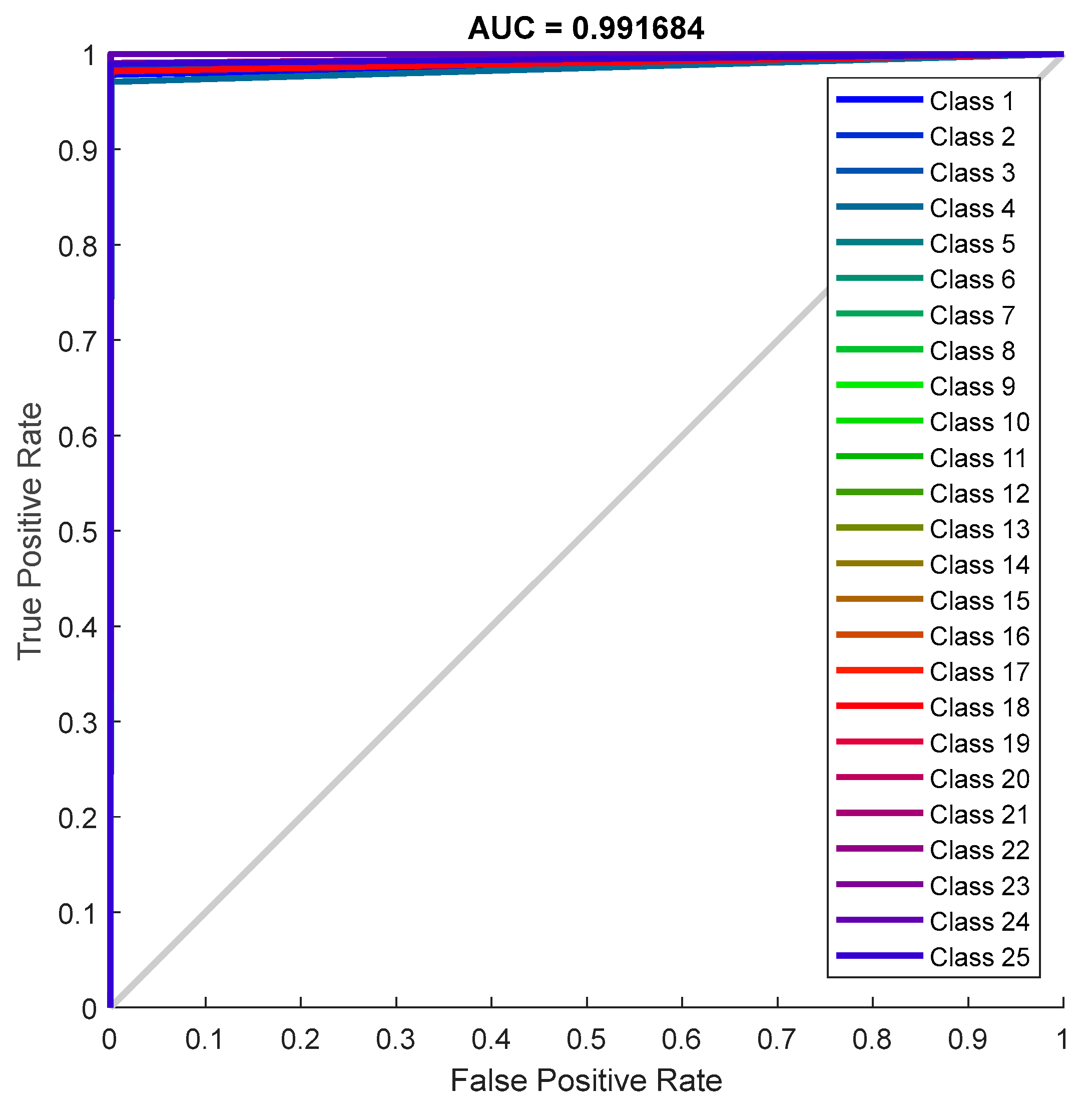
4.3.3. Receiver Operating Characteristic (ROC) Analysis

The receiver operating characteristic (ROC) is one of the metrics used to visualize the improvement of the binary classifier. Through the ROC, the False Positive Rate (FPR) and True Positive Rate (TPR) will be deduced. The curve with a high top-left corner has the best TPR and vice versa. The diagonal line refers to the worst classifier. By these aspects of the ROC, the improvement of the classifier performed by using the suggested system could be deduced, as shown in Figure 7.

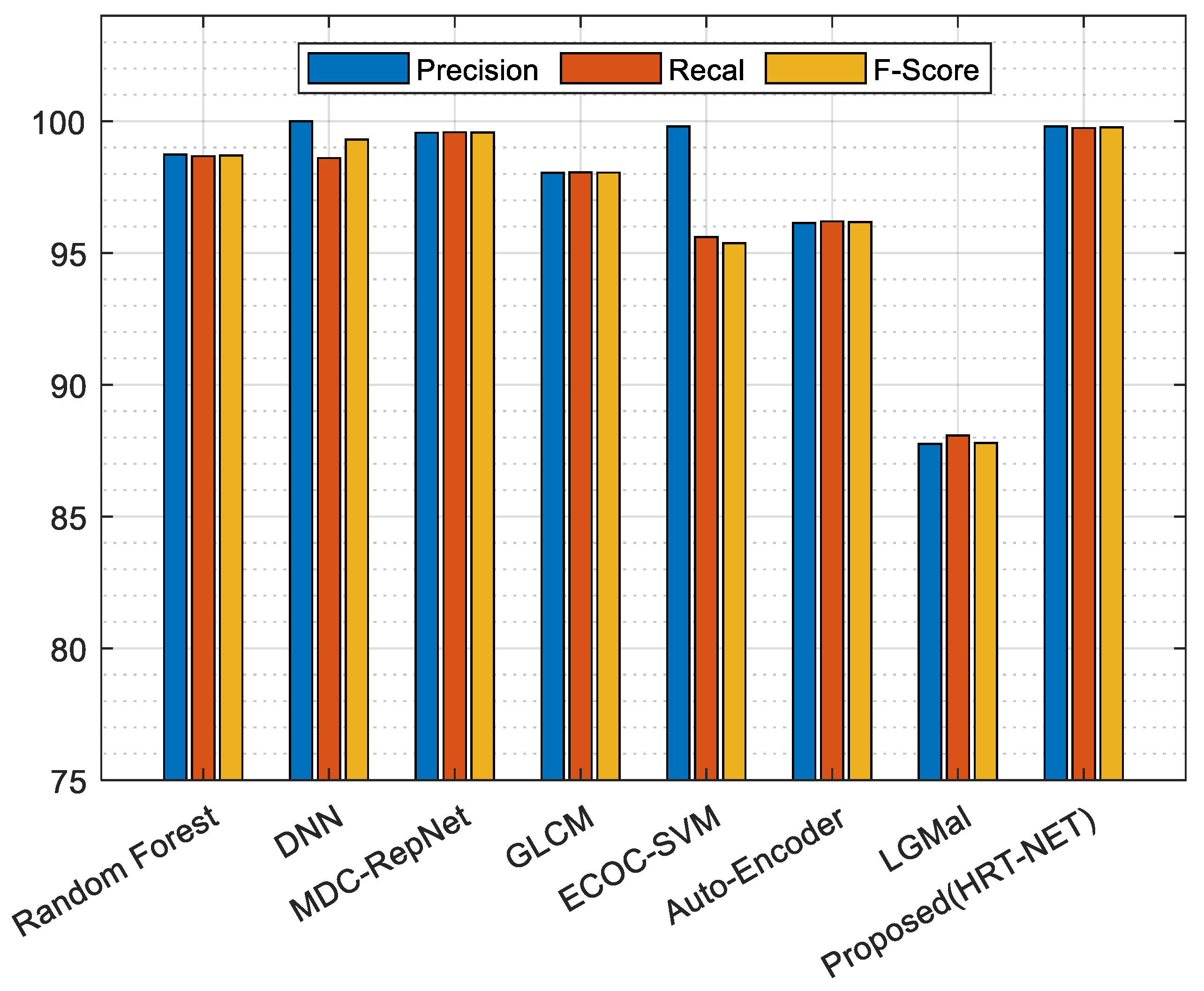
4.3.4. Results Comparison and Discussion

Figure 8 and

Table 2. Comparison of the proposed method with other studies in terms of Precision, Recall, and F1-score criteria.

Methods	Precision	Recall	F1-Score
GLCM [40]	98.04	98.06	98.05
Random Forest [41]	98.74	98.67	98.70
DNN [42]	100	98.60	99.30
MDC-RepNet [43]	99.56	99.58	99.57
ECOC –SVM [44]	99.80	95.6	95.37
Auto Encoder [45]	96.14	96.20	96.17
LGMal [36]	87.76	88.08	87.79
Proposed (HRT-Net-IGOA-Ensemble Learning)	99.80	99.74	99.77

present a comprehensive comparison of the proposed HRT-Net-IGOA-Ensemble Learning approach against other existing methodologies (GLCM, Random Forest, DNN, MDC-RepNet, ECOC-SVM, Auto Encoder) based on Precision, Recall, and F1-score metrics. A detailed analysis of these results clearly highlights the superior performance and efficiency of the presented methodology. The HRT-Net-IGOA-Ensemble Learning approach demonstrates an exceptionally strong and competitive performance, achieving a Precision of 99.80%, Recall of 99.74%, and an F1-score of 99.77%. These figures underscore the model’s high capability in accurately identifying malware instances (high Precision) while simultaneously ensuring a maximum detection rate of all existing malware (high Recall). The resulting high F1-score, as the harmonic mean of Precision and Recall, serves as a comprehensive metric for evaluating the balance between these two, indicating that the presented method achieves an optimal equilibrium. In comparative analysis, methods such as GLCM, Random Forest, LGMal, and Auto Encoder, with F1-scores of 98.05%, 98.70%, 87.79%, and 96.17%, respectively, exhibit comparatively lower performance. This suggests that more traditional methods or simpler deep learning models, when used in isolation, may not be as effective in extracting and differentiating complex malware features with the same level of efficacy as the HRT-Net architecture. The DNN method shows outstanding performance in preventing false positives with a perfect Precision of 100%; however, its Recall is notably lower at 98.60%, implying that it misses a portion of actual malware samples. In contrast, the presented method, while maintaining a very high Precision of 99.80%, achieves a significantly higher Recall of 99.74%. This results in a superior F1-score of 99.77% compared to DNN’s 99.30%, indicating that a better balance is established, offering more comprehensive detection. MDC-RepNet, with an F1-score of 99.57%, emerges as one of the closest competitors to the proposed methodology. Nevertheless, the HRT-Net-IGOA-Ensemble Learning approach consistently maintains a slight edge across all three metrics: Precision (99.80% vs. 99.56%), Recall (99.74% vs. 99.58%), and F1-score (99.77% vs. 99.57%), signifying a more effective optimization in the detection process. The ECOC-SVM method, while achieving a high Precision of 99.80%, identical to the proposed methodology, exhibits a substantially lower Recall at 95.6%. This significant discrepancy in Recall leads to a considerably lower F1-score of 95.37% for ECOC-SVM. This comparison underscores that while ECOC-SVM is highly accurate in its positive predictions, it fails to identify a notable proportion of actual malware (resulting in numerous false negatives), whereas the presented method successfully maintains both very high Precision and Recall simultaneously. In summary, the results presented in Table 2 unequivocally demonstrate that the synergistic combination of the HRT-Net architecture (leveraging ResNet for local features and Transformer for long-range dependencies), the Improved Grasshopper Optimization Algorithm (IGOA) for optimal feature selection, and the Ensemble Learning technique culminates in a malware detection system that either outperforms or delivers unparalleled competitive performance across all measured metrics (Precision, Recall, and F1-score) when compared to the existing methodologies. These findings robustly affirm the effectiveness and comprehensive superiority of the HRT-Net-IGOA-Ensemble Learning approach in addressing complex 25-type malware identification tasks.

Table 3. Comparison of the results.

Authors	Methods	Accuracy
Verma, et al. [40]	GLCM	98.58
Atitallah et al. [41]	Random Forest	98.68
Shaukat et al. [42]	DNN	99.30
Li, Sicong et al. [43]	MDC-RepNet	99.57
Wong, W. et al. [44]	ECOC-SVM	95.01
XIAOFEI XING et al. [45]	Auto Encoder	96.22
Yuhan Chai et al. [36]	LGMal	88.78
-	Proposed (HRT-Net-IGOA-Ensemble Learning)	99.85

compares the performance of the proposed method with other existing approaches in the field of malware classification and detection based on the Accuracy metric. Accuracy is one of the key evaluation criteria for classification models, representing the ratio of correctly classified samples to the total number of samples. A higher accuracy indicates a better model performance in correctly identifying different classes (both malware and benign samples). According to the data presented in the table, the proposed method (HRT-Net-IGOA-Ensemble Learning) achieves the highest accuracy of 99.85%, outperforming all the compared methods. This result highlights the method’s strong ability to learn the distinguishing features of malware samples and accurately classify them. Among the competing methods, MDC-RepNet ranks second with an accuracy of 99.57%, which, while close, still shows a noticeable gap compared to the proposed approach. Similarly, the DNN model achieves an accuracy of 99.30%, which, although acceptable, is approximately 0.5% lower than that of the proposed method—a difference that can be significant in security-sensitive applications such as malware detection, where even slight improvements can substantially reduce risk and detection error. The Random Forest and GLCM methods, with accuracies of 98.68% and 98.58%, respectively, rank lower and, while yielding reasonable results, are not comparable in accuracy to deep learning-based methods. On the other hand, Auto Encoder, ECOC-SVM, and especially LGMal, with accuracies of 96.22%, 95.01%, and 88.78%, respectively, demonstrate weaker performance, which may stem from their limitations in capturing the complex features inherent in malware data.

Overall, the results in Table 3 indicate that the proposed method—by leveraging the deep neural network HRT-Net, the Improved Grasshopper Optimization Algorithm (IGOA), and the Ensemble Learning approach—has successfully extracted powerful features and effectively learned hidden patterns within the data. This superior performance underscores the high reliability of the proposed method for real-world, mission-critical applications in the domain of cybersecurity.

Table 4. Class-based comparison of the results of the proposed method with other methods in terms of the Accuracy criterion.

Classes	GLCM	RF	DNN	MDC-RepNet	ECOC-SVM	Auto Encoder	LGMal	Proposed
C1	100	97.8	100	99.28	91.68	93.7	100	100
C2	97.63	97.8	100	99.28	91.68	100	81.3	100
C3	97.63	100	100	99.28	91.68	100	100	100
C4	97.63	100	98.83	99.28	91.68	93.7	100	100
C5	97.63	97.8	98.83	100	91.68	93.7	81.3	100
C6	97.63	100	100	99.28	100	100	100	100
C7	100	97.8	98.83	99.28	91.68	100	81.3	100
C8	97.63	97.8	100	99.28	91.68	93.7	81.3	100
C9	100	100	98.83	100	100	93.7	100	100
C10	100	100	98.83	99.28	100	100	81.3	100
C11	100	97.8	98.83	100	91.68	93.7	100	100
C12	97.63	97.8	98.83	100	100	93.7	81.3	98.9
C13	97.63	97.8	98.83	100	91.68	93.7	81.3	100
C14	97.63	100	98.83	99.28	100	93.7	81.3	100
C15	100	100	98.83	99.28	100	93.7	81.3	100
C16	97.63	97.8	100	99.28	91.68	93.7	100	100
C17	97.63	97.8	98.83	100	91.68	100	81.3	100
C18	100	97.8	98.83	100	91.68	100	81.3	100
C19	100	97.8	98.83	99.28	100	93.7	100	100
C20	97.63	100	98.83	100	91.68	93.7	81.3	100
C21	97.63	97.8	100	100	91.68	100	100	100
C22	97.63	100	100	100	91.68	93.7	100	100
C23	100	97.8	98.83	99.28	100	100	81.3	100
C24	97.63	97.8	100	99.28	100	93.7	81.3	98.3
C25	100	100	100	99.28	100	100	81.3	98.9
Av.	98.58	98.68	99.30	99.57	95.01	96.22	88.78	99.85

presents a class-specific performance comparison in terms of classification accuracy between the proposed method and several established techniques, including GLCM, RF, DNN, MDC-RepNet, ECOC-SVM, Auto Encoder, and LGMal. As evidenced in the table, the proposed method consistently outperforms the competing approaches by achieving a perfect classification accuracy (100%) in 22 out of 25 classes. In the remaining three classes (C12, C24, and C25), the method still maintains exceptionally high accuracy values of 98.9%, 98.3%, and 98.9%, respectively. This results in an overall average accuracy of 99.85%, the highest among all compared methods. While other methods such as DNN (99.30%) and MDC-RepNet (99.57%) also demonstrate competitive average performance, they fail to deliver consistent results across all classes. For instance, DNN shows accuracy drops in several classes (e.g., 98.83%), indicating potential limitations in generalizing across diverse data distributions. Similarly, methods like GLCM and RF show relatively high average accuracy (98.58% and 98.68%, respectively) but still lag behind in class-level precision and stability. More notably, the ECOC-SVM and LGMal methods underperform in terms of both per-class accuracy and average performance, with the latter achieving the lowest mean accuracy of 88.78%. This inconsistency in classification results across classes underscores the limited robustness of these techniques in handling complex multi-class scenarios.

The proposed method’s superior and consistent performance highlights its effectiveness in learning discriminative features and maintaining classification integrity across a wide range of class instances. This level of class-specific performance is particularly critical in real-world applications where class imbalance or subtle inter-class variations can significantly impact the reliability of classification systems (such as security systems) detection. In conclusion, the results in Table 4 clearly demonstrate the dominance of the proposed method in both overall and class-specific performance, making it a highly reliable and generalizable solution for multi-class classification tasks.

To practically validate the improvement in the computational complexity of the proposed method,

Table 5. Comparing the computational complexity.

Methods	Training Time (min)	Testing Time (ms)
GLCM [40]	14.6	43
Random Forest [41]	13.4	40
DNN [42]	20.3	92
MDC-RepNet [43]	22.6	104
ECOC-SVM [44]	15.7	49
Auto Encoder [45]	18.1	78
LGMal [36]	16.9	56
Proposed (HRT-Net + IGOA feature selection + Ensemble Learning)	12.3	36

presents a comparative analysis of its computational performance against existing studies. The evaluation metrics include training time and testing time. All methods were tested under identical hardware conditions (Intel i7 processor, 16 GB RAM) and on the Malimg dataset.

Due to the use of optimal feature selection in the proposed method, which leads to a reduction in feature dimensionality, the classification process requires significantly less time for malware detection. This dimensionality reduction not only accelerates the training phase but also substantially decreases the time required for predicting new samples. Specifically, the testing time for classifying a single sample was measured at only 36 milliseconds, demonstrating the method’s suitability for real-time applications.

It is important to note that training a model typically involves learning from a large set of data, so training time is naturally much longer than testing time. However, during the testing phase, the network only needs to process a single input to make a decision, which requires significantly less time. Furthermore, since the training process is performed only once, and the trained model can be reused to classify any number of new samples without retraining, testing time becomes a much more critical metric for designing online detection systems. Overall, the results in Table 5 confirm that the combination of optimal feature selection and Ensemble Learning has remarkably improved the computational performance of the proposed method, making it an efficient and practically deployable solution for real-world malware detection systems.

5. Conclusions

Malware is any kind of program whose primary intended function is to have a negative impact on the operation of a computer system, its users or network. It can be in any form, whether in text documents, an executable, or any other type of software. In general, malware can be classified as worms, viruses, rootkits, ransomware, adware/spyware, Trojans, scareware, bots, potentially unwanted programs (PUPs), and other damaging programs. As more and more people go online, the rate and severity of such attacks are likely to rise. In this study, the HRT-Net was proposed as a new type of network for classifying 25 types of malware. First, the images of malware were augmented through HRT-Net, where ResNet encoded local patterns and the Transformer captured long-range dependencies and contextual patterns. The features extracted were then concatenated to form a dataset with all the compressed features used for analysis. The dynamic mutation factor and the dynamic inertia motion factors were then used in the Improved Grasshopper Optimization Algorithm (IGOA) to identify an optimal subset that decreases computational cost without compromising on the relevant information. Lastly, the Ensemble Learning technique was used for classification purposes, even if it is quite time consuming. Hence, relative to the current article, an accuracy estimate of 99.7% established the usefulness of HRT-Net in dealing with complex malware identification tasks.

6. Future Work

Building upon the promising results achieved by the HRT-Net in classifying 25 types of malware with a high accuracy of 99.7%, our future research will focus on several key areas to further enhance its capabilities and address existing challenges.

• Firstly, recognizing that the current Ensemble Learning technique utilized is “quite time consuming,” a significant focus will be placed on optimizing the computational efficiency of the classification phase. This involves exploring more lightweight ensemble methodologies, investigating parallel processing techniques, or developing adaptive ensemble strategies that dynamically select models based on real-time constraints, thereby reducing detection latency without compromising accuracy.
• Secondly, while HRT-Net effectively extracts features from malware images for static analysis, a crucial next step is to extend its capabilities to dynamic analysis. This involves integrating behavioral features derived from API calls, system logs, or network traffic. A hybrid static-dynamic analysis approach could provide a more comprehensive understanding of malware behavior, significantly enhancing detection robustness against advanced obfuscation techniques and zero-day threats.
• Furthermore, we aim to rigorously evaluate the HRT-Net’s performance against significantly larger and more diverse real-world malware datasets, including those containing a higher volume of previously unseen (zero-day) and highly evasive samples. This will allow for a more robust assessment of its scalability and generalization capabilities in real-world cybersecurity scenarios.
• Finally, two additional critical directions for future work include assessing the HRT-Net’s resilience against adversarial attacks specifically designed to evade deep learning-based detectors and enhancing the interpretability and explainability of the model’s decisions, providing security analysts with actionable insights into the malicious characteristics identified by the system.

References

1. Ferdous, J.; Islam, R.; Mahboubi, A.; Islam, M.Z. A Survey on ML Techniques for Multi-Platform Malware Detection: Securing PC, Mobile Devices, IoT, and Cloud Environments. Sensors 2025, 25, 1153. [Google Scholar] [CrossRef] [PubMed]
2. Kumar, S.S.; Stephen, S.; Rumysia, M.S. Rootkit detection using deep learning: A comprehensive survey. In Proceedings of the 10th International Conference on Communication and Signal Processing (ICCSP), Melmaruvathur, India, 12–14 April 2024; IEEE: New York, NY, USA, 2024. [Google Scholar]
3. Sharma, T.; Patni, K.; Li, Z.; Trajković, L. Deep echo state networks for detecting internet worm and ransomware attacks. In Proceedings of the IEEE International Symposium on Circuits and Systems (ISCAS), Monterey, CA, USA, 21–25 May 2023; IEEE: New York, NY, USA, 2023. [Google Scholar]
4. Zhan, D.; Xu, K.; Liu, X.; Han, T.; Pan, Z.; Guo, S. Practical clean-label backdoor attack against static malware detection. Comput. Secur. 2025, 150, 104280. [Google Scholar] [CrossRef]
5. Ahila, A.; Lakshmi, A.A.; Ragavendran, N.; Purushothaman, K.E.; Maheswari, G.U.; Saravanakumar, R. Advancements in Cybersecurity Using Deep Learning Techniques Attack Detection for Trojan Horses. In Proceedings of the International Conference on Electrical Electronics and Computing Technologies (ICEECT), Greater Noida, India, 29–31 August 2024; IEEE: New York, NY, USA, 2024; Volume 1. [Google Scholar]
6. Almoqbil, A.H.N. Anomaly detection for early ransomware and spyware warning in nuclear power plant systems based on FusionGuard. Int. J. Inf. Secur. 2024, 23, 2377–2394. [Google Scholar] [CrossRef]
7. Gautam, A.; Rahimi, N. Viability of machine learning in android scareware detection. Proceedings of 38th International Conference on Computers and Their Applications, Online, 20–22 March 2023; Volume 91, pp. 19–26. [Google Scholar]
8. Velasco Mata, J. Botnet Activity Spotting with Artificial Intelligence: Efficient Bot Malware Detection and Social Bot Identification. Ph.D. Thesis, Universidad de León, León, Spain, 2023. [Google Scholar]
9. Bensaoud, A.; Kalita, J.; Bensaoud, M. A survey of malware detection using deep learning. Mach. Learn. Appl. 2024, 16, 100546. [Google Scholar] [CrossRef]
10. Pang, S.; Wen, J.; Liang, S.; Huang, B. FICConvNet: A Privacy-Preserving Framework for Malware Detection Using CKKS Homomorphic Encryption. Electronics 2025, 14, 1982. [Google Scholar] [CrossRef]
11. Silfiah, R.I.; Sulatri, K.; Ismail, Y. Legal Protection of Consumers with Online Transactions. J. Law Politic Humanit. 2024, 4, 2584–2595. [Google Scholar]
12. Ighomereho, O.S.; Afolabi, T.S.; Oluwakoya, A.O. Impact of E-service quality on customer satisfaction: A study of internet banking for general and maritime services in Nigeria. J. Financ. Serv. Mark. 2023, 28, 488–501. [Google Scholar] [CrossRef]
13. Laghari, A.A.; Jumani, A.K.; Laghari, R.A.; Li, H.; Karim, S.; Khan, A.A. Unmanned aerial vehicles advances in object detection and communication security review. Cogn. Robot. 2024, 4, 128–141. [Google Scholar] [CrossRef]
14. Zhukabayeva, T.; Zholshiyeva, L.; Karabayev, N.; Khan, S.; Alnazzawi, N. Cybersecurity Solutions for Industrial Internet of Things–Edge Computing Integration: Challenges, Threats, and Future Directions. Sensors 2025, 25, 213. [Google Scholar] [CrossRef]
15. Alhogail, A.; Alharbi, R.A. Effective ML-Based Android Malware Detection and Categorization. Electronics 2025, 14, 1486. [Google Scholar] [CrossRef]
16. Lee, J.; Kim, J.; Jeong, H.; Lee, K. A Machine Learning-Based Ransomware Detection Method for Attackers’ Neutralization Techniques Using Format-Preserving Encryption. Sensors 2025, 25, 2406. [Google Scholar] [CrossRef]
17. Tumuluru, P.; LRBurra MVVReddy SSudarsa, S.Y.; Reddy, A.L.A. APMWMM: Approach to Probe Malware on Windows Machine using Machine Learning. In Proceedings of the 2022 International Conference on Applied Artificial Intelligence and Computing (ICAAIC), Salem, India, 9–11 May 2022; pp. 614–619. [Google Scholar] [CrossRef]
18. Duby, A.; Taylor, T.; Bloom, G.; Zhuang, Y. Detecting and Classifying Self-Deleting Windows Malware Using Prefetch Files. In Proceedings of the 2022 IEEE 12th Annual Computing and Communication Workshop and Conference (CCWC), Las Vegas, NV, USA, 26–29 January 2022; pp. 745–751. [Google Scholar] [CrossRef]
19. Duby, A.; Taylor, T.; Bloom, G.; Zhuang, Y. Evaluating Feature Robustness for Windows Malware Family Classification. In Proceedings of the 2022 International Conference on Computer Communications and Networks (ICCCN), Honolulu, HI, USA, 25–27 July 2022; pp. 1–10. [Google Scholar] [CrossRef]
20. Ficco, M. Malware Analysis by Combining Multiple Detectors and Observation Windows. IEEE Trans. Comput. 2022, 71, 1276–1290. [Google Scholar] [CrossRef]
21. Namita; Prachi; Sharma, P. Windows Malware Detection using Machine Learning and TF-IDF Enriched API Calls Information. In Proceedings of the 2022 Second International Conference on Computer Science, Engineering and Applications (ICCSEA), Gunupur, India, 8 September 2022; pp. 1–6. [Google Scholar] [CrossRef]
22. Nawshin, F.; Gad, R.; Unal, D.; Al-Ali, A.K.; Suganthan, P.N. Malware detection for mobile computing using secure and privacy-preserving machine learning approaches: A comprehensive survey. Comput. Electr. Eng. 2024, 117, 109233. [Google Scholar] [CrossRef]
23. Uysal, D.T.; Yoo, P.D.; Taha, K. Data-Driven Malware Detection for 6G Networks: A Survey From the Perspective of Continuous Learning and Explainability via Visualisation. IEEE Open J. Veh. Technol. 2023, 4, 61–71. [Google Scholar] [CrossRef]
24. Gopinath, M.; Sethuraman, S.C. A comprehensive survey on deep learning based malware detection techniques. Comput. Sci. Rev. 2023, 47, 100529. [Google Scholar]
25. Gaurav, A.; Gupta, B.B.; Panigrahi, P.K. A Comprehensive Survey on Machine Learning Approaches for Malware Detection in IoT-Based Enterprise Information System. Enterp. Inf. Syst. 2022, 17, 1–25. [Google Scholar] [CrossRef]
26. Yadav, P.; Menon, N.; Ravi, V.; Vishvanathan, S.; Pham, T.D. EfficientNet Convolutional Neural Networks-Based Android Malware Detection. Comput. Secur. 2022, 115, 102622. [Google Scholar] [CrossRef]
27. Rey, V.; Sánchez, P.M.S.; Celdrán, A.H.; Bovet, G. Federated Learning for Malware Detection in IoT Devices. Comput. Netw. 2022, 204, 108693. [Google Scholar] [CrossRef]
28. Cai, H. Assessing and Improving Malware Detection Sustainability through App Evolution Studies. ACM Trans. Softw. Eng. Methodol. 2020, 29, 1–28. [Google Scholar] [CrossRef]
29. Xu, K.; Li, Y.; Deng, R.; Chen, K.; Xu, J. DroidEvolver: Self-Evolving Android Malware Detection System. In Proceedings of the IEEE European Symposium on Security and Privacy (EuroS&P), Vienna, Austria, 8–12 June 2019; pp. 47–62. [Google Scholar]
30. Gibert, D.; Mateu, C.; Planes, J. A Hierarchical Convolutional Neural Network for Malware Classification. In Proceedings of the 2019 International Joint Conference on Neural Networks (IJCNN), Budapest, Hungary, 14–19 July 2019; pp. 1–8. [Google Scholar] [CrossRef]
31. Sharma, A.; Malacaria, P.; Khouzani, M.H.R. Malware Detection Using 1-Dimensional Convolutional Neural Networks. In Proceedings of the 2019 IEEE European Symposium on Security and Privacy Workshops (EuroS&PW), Stockholm, Sweden, 17–19 June 2019; pp. 247–256. [Google Scholar] [CrossRef]
32. Shiva Darshan, S.L.; Jaidhar, C.D. Windows Malware Detector Using Convolutional Neural Network Based on Visualization Images. IEEE Trans. Emerg. Top. Comput. 2019, 9, 1057–1069. [Google Scholar] [CrossRef]
33. Shaukat, K.; Luo, S.; Varadharajan, V. A Novel Deep Learning-Based Approach for Malware Detection. Eng. Appl. Artif. Intell. 2023, 122, 106030. [Google Scholar] [CrossRef]
34. Aslan, O.; Yilmaz, A.A. A New Malware Classification Framework Based on Deep Learning Algorithms. IEEE Access 2021, 9, 87936–87951. [Google Scholar] [CrossRef]
35. Maniriho, P.; Mahmood, A.N.; Chowdhury, M.J.M. API-MalDetect: Automated Malware Detection Framework for Windows Based on API Calls and Deep Learning Techniques. J. Netw. Comput. Appl. 2023, 218, 103704. [Google Scholar] [CrossRef]
36. Chai, Y.; Qiu, J.; Su, S.; Zhu, C.; Yin, L.; Tian, Z. LGMal: A Joint Framework Based on Local and Global Features for Malware Detection. In Proceedings of the International Wireless Communications and Mobile Computing Conference (IWCMC), Limassol, Cyprus, 15–19 June 2020; pp. 463–468. [Google Scholar] [CrossRef]
37. Peng, J.; Kang, S.; Ning, Z.; Deng, H.; Shen, J.; Xu, Y.; Zhang, J.; Zhao, W.; Li, X.; Gong, W.; et al. Residual Convolutional Neural Network for Predicting Response of Transarterial Chemoembolization in Hepatocellular Carcinoma from CT Imaging. Eur. Radiol. 2020, 30, 413–424. [Google Scholar] [CrossRef] [PubMed]
38. Obaid, Z.H.; Mirzaei, B.; Darroudi, A. An Efficient Automatic Modulation Recognition Using Time–Frequency Information Based on Hybrid Deep Learning and Bagging Approach. Knowl. Inf. Syst. 2024, 66, 2607–2624. [Google Scholar] [CrossRef]
39. Malimg Malware Dataset. Available online: https://www.kaggle.com/datasets/manmandes/malimg (accessed on 1 May 2025).
40. Verma, V.; Muttoo, S.K.; Singh, V.B. Multiclass Malware Classification via First- and Second-Order Texture Statistics. Comput. Secur. 2020, 97, 101895. [Google Scholar] [CrossRef]
41. Atitallah, S.B.; Driss, M.; Almomani, I. A Novel Detection and Multi-Classification Approach for IoT-Malware Using Random Forest Voting of Fine-Tuning Convolutional Neural Networks. Sensors 2022, 22, 4302. [Google Scholar] [CrossRef]
42. Shaukat, K.; Luo, S.; Varadharajan, V. A Novel Machine Learning Approach for Detecting First-Time-Appeared Malware. Eng. Appl. Artif. Intell. 2024, 131, 107801. [Google Scholar] [CrossRef]
43. Li, S.; Wang, J.; Song, Y.; Wang, S.; Wang, Y. A Lightweight Model for Malicious Code Classification Based on Structural Reparameterisation and Large Convolutional Kernels. Int. J. Comput. Intell. Syst. 2024, 17, 30. [Google Scholar] [CrossRef]
44. Wong, W.; Juwono, F.H.; Apriono, C. Vision-Based Malware Detection: A Transfer Learning Approach Using Optimal ECOC-SVM Configuration. IEEE Access 2021, 9, 159262–159270. [Google Scholar] [CrossRef]
45. Xing, X.; Jin, X.; Elahi, H.; Jiang, H.; Wang, G. A Malware Detection Approach Using Autoencoder in Deep Learning. IEEE Access 2022, 10, 25696–25706. [Google Scholar] [CrossRef]
Figure 1. Diagram of the suggested method.
Electronics 14 02741 g001
Figure 2. The Hybrid Resnet Transformer Network Structure (HRT-Net).
Electronics 14 02741 g002
Figure 3. Classification with Ensemble Learning technique.
Electronics 14 02741 g003
Figure 4. Different types of malware class.
Electronics 14 02741 g004
Figure 5. Ensemble Learning convergence curve against number of learners.
Electronics 14 02741 g005
Figure 6. Confusion matrix.
Electronics 14 02741 g006
Figure 7. ROC curve.
Electronics 14 02741 g007
Figure 8. Comparison of results in terms of Precision, Recall, and F1-score criteria.
Electronics 14 02741 g008