
Modified Dual Hierarchical Terminal Sliding Mode Control Design for Two-Wheeled Self-Balancing Robot


Abstract
1. Introduction
- A hierarchical sliding mode control (HSMC) scheme is combined with terminal sliding mode control (TSMC) to address the underactuated control problem of the two-wheeled self-balancing robot (TWSBR), resulting in a dual-terminal sliding mode control (DTSMC) law. Furthermore, a modified dual hierarchical terminal sliding mode control (MDHTSMC) scheme is designed based on the duality concept, with stability rigorously verified through Lyapunov theory.
- A modified dual hierarchical terminal sliding mode control (MDHTSMC) scheme is proposed for the TWSBR nonlinear system, accounting for disturbances and uncertainties. Using Lyapunov theory, finite-time convergence on the newly defined MDHTSMC surface is proven, and the arrival and sliding times are explicitly calculated.
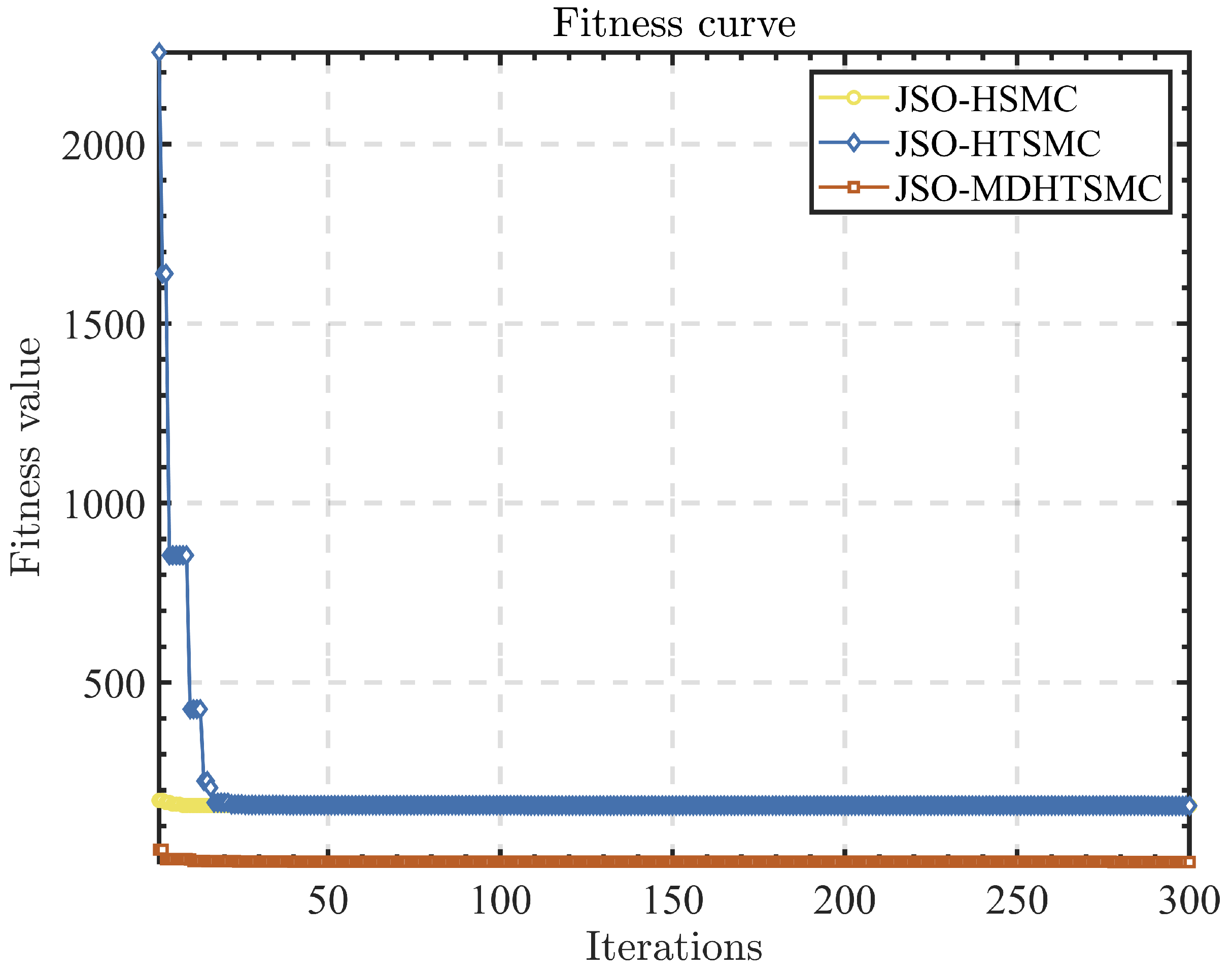
- The Jellyfish Search Optimization (JSO) algorithm is employed to minimize the integral of the time-weighted absolute error (ITAE) by adjusting the x and parameters of the TWSBR, achieving optimal control parameters. These parameters are subsequently fine-tuned for enhanced optimization.
2. Preliminary
2.1. Dynamic Models
2.2. Actuated and Underactuated Subsystems
2.2.1. -Subsystem
2.2.2. -Subsystem
3. Modified Dual Hierarchical Terminal SMC
3.1. Dynamic Model
3.2. Hierarchical Terminal Sliding Mode Control (HTSMC)
3.3. Dual Hierarchical Terminal SMC (DHTSMC)
3.4. MDHTSM Controller Design for TWSBR
4. Simulation Result
4.1. Optimization Algorithm
4.2. Parameter Tuning
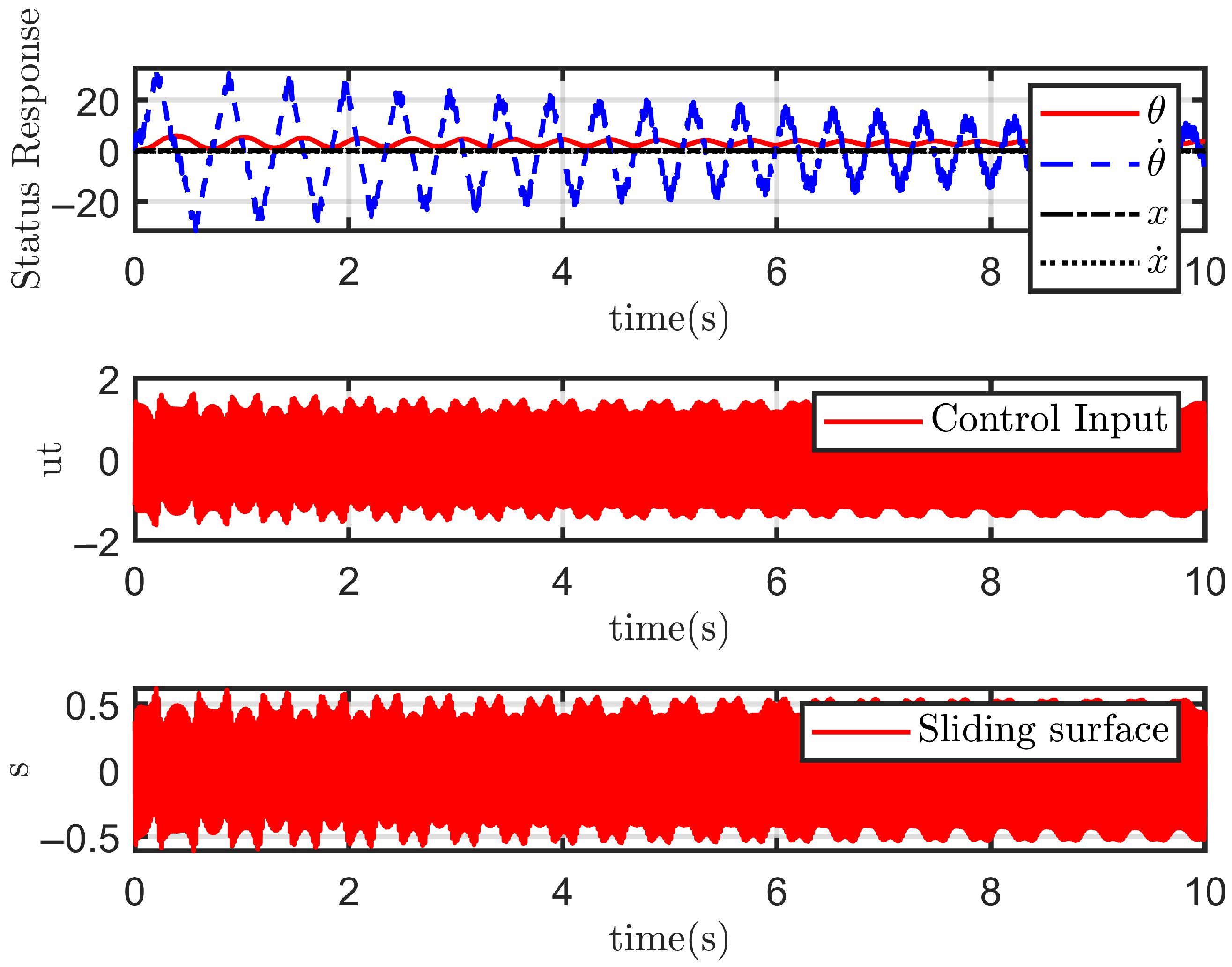
- The performance of each sliding mode controller under ideal, disturbance-free conditions;
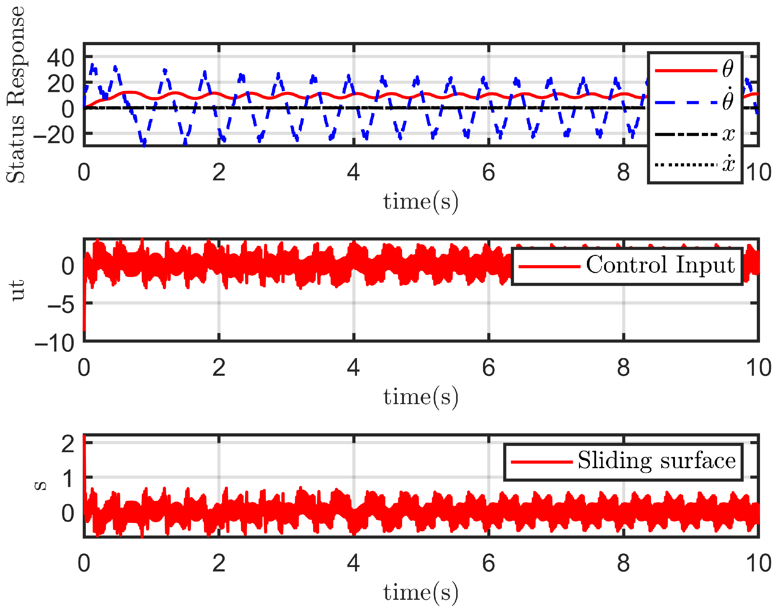
- The performance of each sliding mode controller in the presence of disturbances .
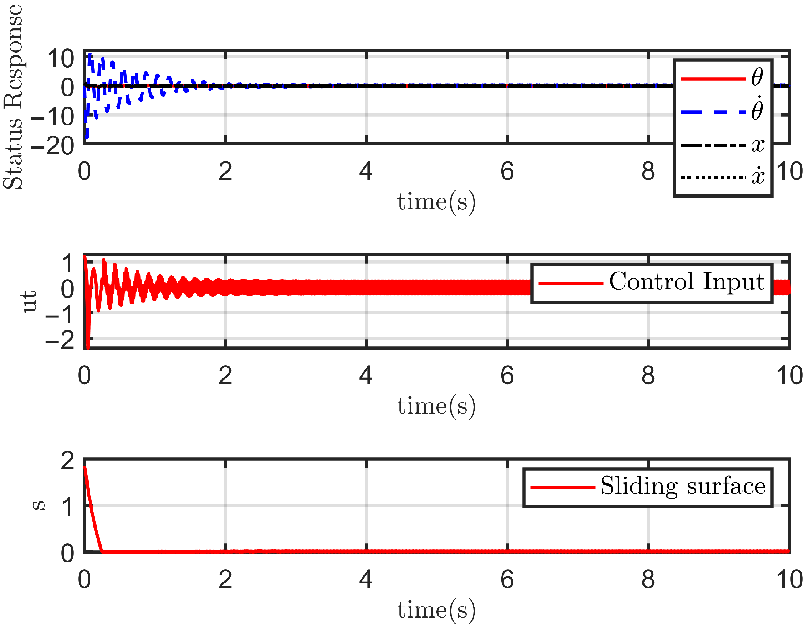
4.2.1. Case 1: Ideal State
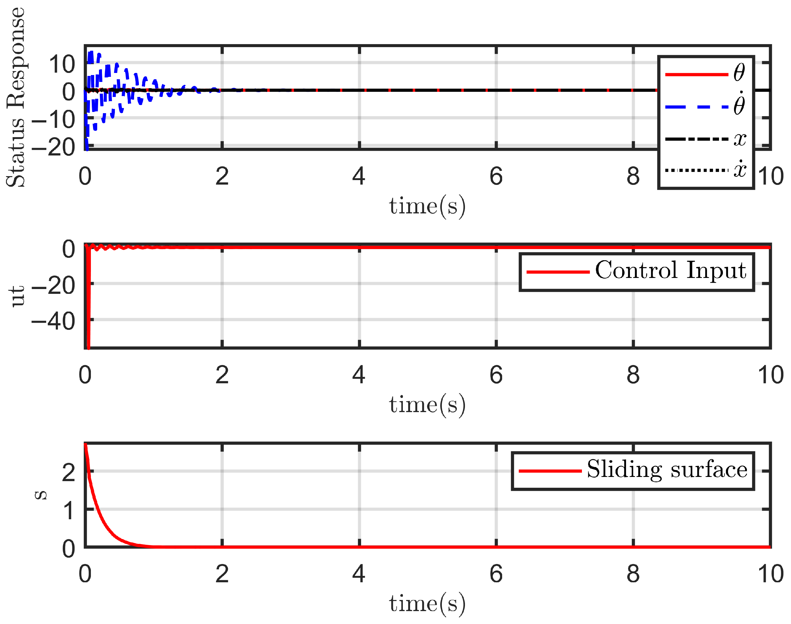
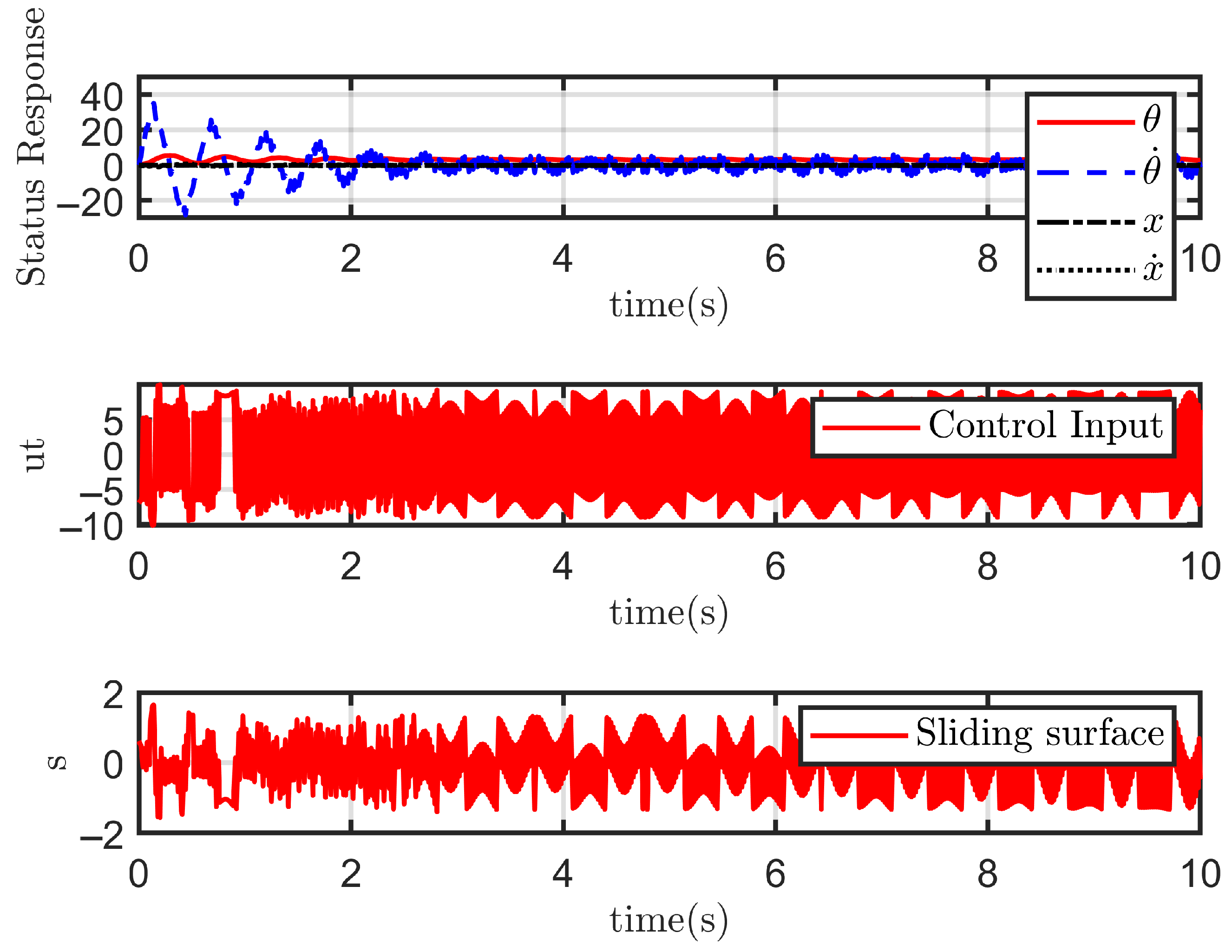
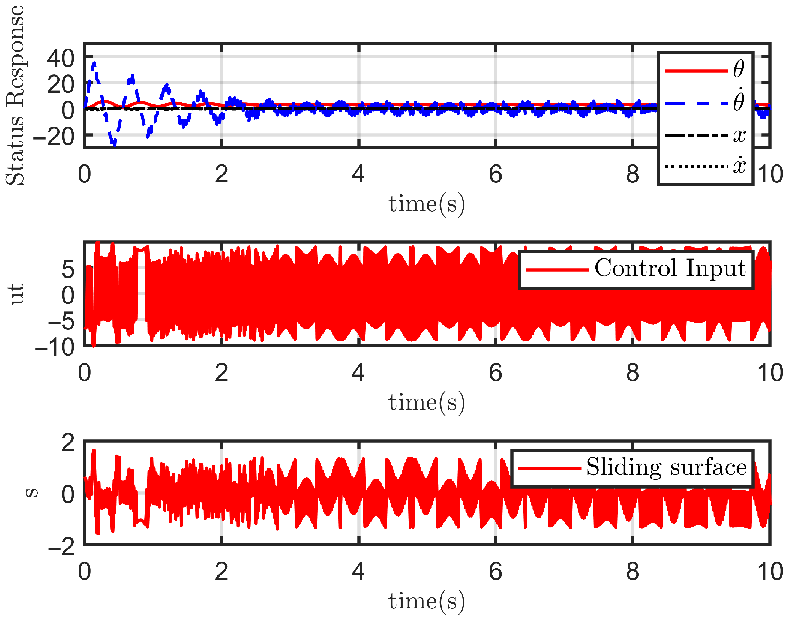
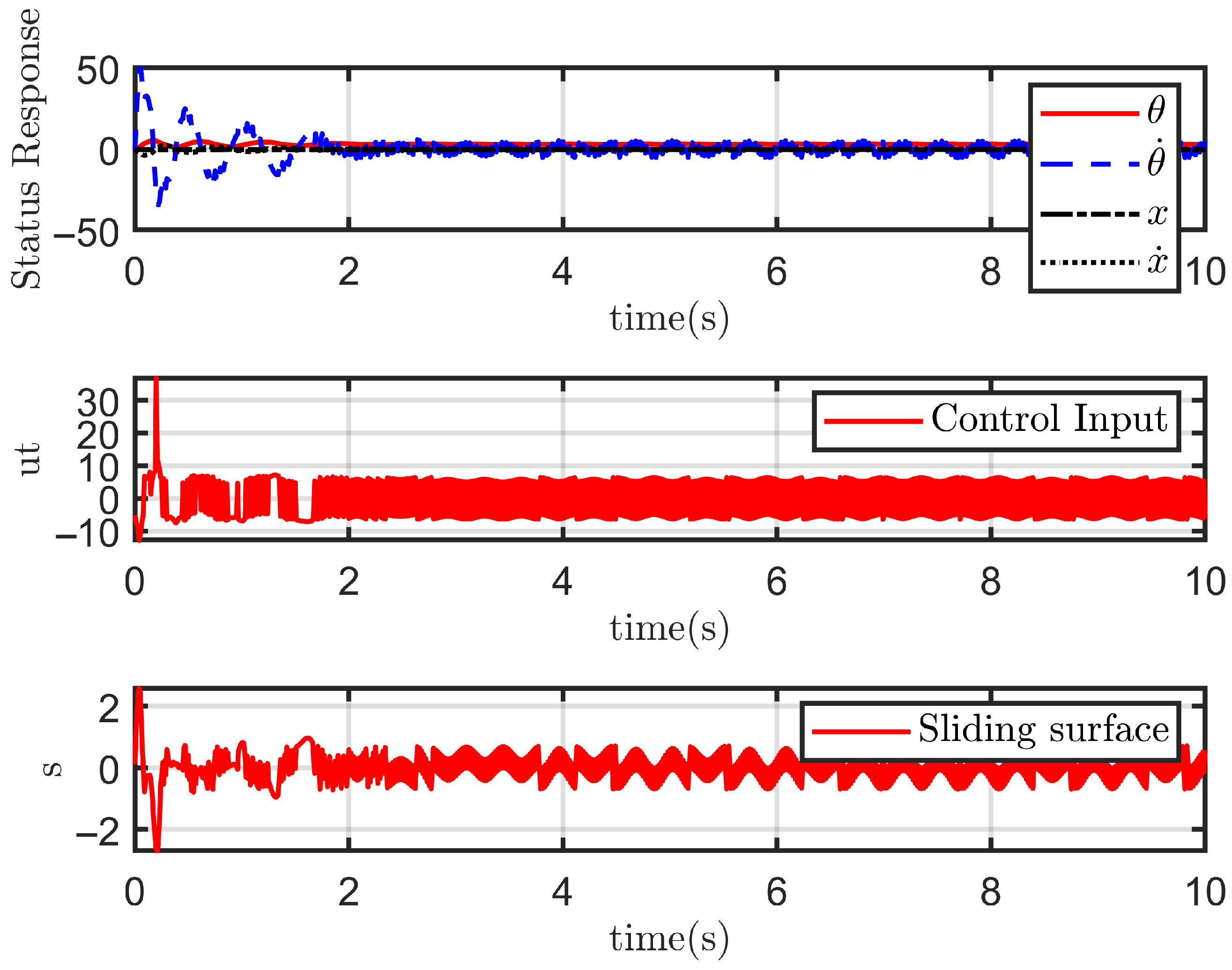
4.2.2. Case 2: With Disturbance
4.3. Indicator Evaluation
5. Conclusions and Future Work
Author Contributions
Funding
Institutional Review Board Statement
Informed Consent Statement
Data Availability Statement
Acknowledgments
Conflicts of Interest
Abbreviations
| TWSBR | Two-Wheeled Self-Balancing Robot |
| SMC | Sliding Mode Control |
| TSMC | Terminal Sliding Mode Control |
| HSMC | Hierarchical Sliding Mode Control |
| HTSMC | Hierarchical Terminal Sliding Mode Control |
| DHTSMC | Dual Hierarchical Terminal Sliding Mode Control |
| MDHTSMC | Modified Dual Hierarchical Terminal Sliding Mode Control |
| JSO | Jellyfish Search Optimization |
| ITAE | Integral of Time-weighted Absolute Error |
| LQR | Linear Quadratic Regulator |
| PD | Proportional-Derivative |
Appendix A
References
- Zhang, S.; Yao, J.; Wang, Y.; Liu, Z.; Xu, Y.; Zhao, Y. Design and motion analysis of reconfigurable wheel-legged mobile robot. Def. Technol. 2022, 18, 1023–1040. [Google Scholar] [CrossRef]
- Rubio, F.; Valero, F.; Llopis-Albert, C. A review of mobile robots: Concepts, methods, theoretical framework, and applications. Int. J. Adv. Robot. Syst. 2019, 16, 1–22. [Google Scholar] [CrossRef]
- Olmez, Y.; Koca, G.O.; Akpolat, Z.H. Clonal selection algorithm based control for two-wheeled self-balancing mobile robot. Simul. Model. Pract. Theory Int. J. Fed. Eur. Simul. Soc. 2022, 118, 102552. [Google Scholar] [CrossRef]
- Guo, Y.; Guo, J.; Liu, L.; Liu, Y.; Leng, J. Bioinspired multimodal soft robot driven by a single dielectric elastomer actuator and two flexible electroadhesive feet. Extrem. Mech. Lett. 2022, 53, 101720. [Google Scholar] [CrossRef]
- Khan, M.B.; Chuthong, T.; Do, C.D.; Thor, M.; Billeschou, P.; Larsen, J.C.; Manoonpong, P. icrawl: An inchworm-inspired crawling robot. IEEE Access 2020, 8, 200655–200668. [Google Scholar] [CrossRef]
- Wang, P.; Tang, Q.; Sun, T.; Dong, R. Research on stability of the four-wheeled robot for emergency obstacle avoidance on the slope. Recent Pat. Eng. 2021, 15, 14–28. [Google Scholar] [CrossRef]
- Nker, F. Proportional controlled moment of gyroscope for two-wheeled self-balancing robot. J. Vib. Control 2021, 28, 2310–2318. [Google Scholar] [CrossRef]
- Voth, D. Segway to the future [autonomous mobile robot]. IEEE Intell. Syst. 2005, 20, 5–8. [Google Scholar] [CrossRef]
- Delgado-Spíndola, A.; Campa, R.; Bugarin, E.; Soto, I. Design and real-time implementation of a nonlinear regulation controller for the rmp-100 segway twip. Mechatronics 2021, 79, 102668. [Google Scholar] [CrossRef]
- Zhao, J.; Cui, X.; Zhu, Y.; Tang, S. A new self-reconfigurable modular robotic system ubot: Multi-mode locomotion and self-reconfiguration. In Proceedings of the 2011 IEEE International Conference on Robotics and Automation, Shanghai, China, 9–13 May 2011; IEEE: Piscataway, NJ, USA, 2011; pp. 1020–1025. [Google Scholar] [CrossRef]
- Cui, X.; Zhu, Y.; Zhao, J.; Piao, S.; Yang, E. Bio-inspired locomotion control for ubot self-reconfigurable modular robot. In Proceedings of the 2023 International Conference on Control, Automation and Diagnosis (ICCAD), Rome, Italy, 10–12 May 2023; IEEE: Piscataway, NJ, USA, 2023; pp. 1–6. [Google Scholar] [CrossRef]
- Gao, D.Y.; Han, P.W.; Zhang, D.S.; Lu, Y.J. Study of sliding mode control in self-balancing two-wheeled inverted car. Appl. Mech. Mater. 2013, 241, 2000–2003. [Google Scholar] [CrossRef]
- Jmel, I.; Dimassi, H.; Hadj-Said, S.; M’Sahli, F. Sliding mode control for two wheeled inverted pendulum under terrain inclination and disturbances. In Proceedings of the 2021 9th International Conference on Systems and Control (ICSC), Caen, France, 24–26 November 2021; IEEE: Piscataway, NJ, USA, 2021; pp. 467–471. [Google Scholar] [CrossRef]
- Ghahremani, A.; Khalaji, A.K. Simultaneous regulation and velocity tracking control of a two-wheeled self-balancing robot. In Proceedings of the 2023 International Conference on Control, Automation and Diagnosis (ICCAD), Rome, Italy, 10–12 May 2023; IEEE: Piscataway, NJ, USA, 2023; pp. 1–6. [Google Scholar] [CrossRef]
- Arani, M.S.; Orimi, H.E.; Xie, W.-F.; Hong, H. Comparison of Sliding Mode Controller and State Feedback Controller Having Linear Quadratic Regulator (lqr) on a Two-Wheel Inverted Pendulum Robot: Design and Experiments. 2018. Available online: http://hdl.handle.net/10315/35251 (accessed on 30 June 2025).
- Sinha, A.; Prasoon, P.; Bharadwaj, P.K.; Ranasinghe, A.C. Nonlinear autonomous control of a two-wheeled inverted pendulum mobile robot based on sliding mode. In Proceedings of the 2015 International Conference on Computational Intelligence and Networks, Odisha, India, 12–13 January 2015; IEEE: Piscataway, NJ, USA, 2015; pp. 52–57. [Google Scholar] [CrossRef]
- Yih, C.-C. Sliding-mode velocity control of a two-wheeled self-balancing vehicle. Asian J. Control 2014, 16, 1880–1890. [Google Scholar] [CrossRef]
- Wang, L.; Lei, J. Research on self-balancing control for upright vehicle with two wheels based on sliding mode control. In Proceedings of the 2017 International Conference on Computer Technology, Electronics and Communication (ICCTEC), Dalian, China, 19–21 December 2017; IEEE: Piscataway, NJ, USA, 2017; pp. 1192–1195. [Google Scholar] [CrossRef]
- Yang, Y.; Yan, X.; Sirlantzis, K.; Howells, G. Regular form-based sliding mode control design on a two-wheeled inverted pendulum. Int. J. Model. Identif. Control 2021, 37, 312–320. [Google Scholar] [CrossRef]
- Fukushima, H.; Muro, K.; Matsuno, F. Sliding-mode control for transformation to an inverted pendulum mode of a mobile robot with wheel-arms. IEEE Trans. Ind. Electron. 2014, 62, 4257–4266. [Google Scholar] [CrossRef]
- Durdevic, P.; Yang, Z. Hybrid control of a two-wheeled automatic-balancing robot with backlash feature. In Proceedings of the 2013 IEEE International Symposium on Safety, Security, and Rescue Robotics (SSRR), Linkoping, Sweden, 21–26 October 2013; IEEE: Piscataway, NJ, USA, 2013; pp. 1–6. [Google Scholar] [CrossRef]
- Irfan, S.; Mehmood, A.; Razzaq, M.T.; Iqbal, J. Advanced sliding mode control techniques for inverted pendulum: Modelling and simulation. Eng. Sci. Technol. Int. J. 2018, 21, 753–759. [Google Scholar] [CrossRef]
- Zheng, N.; Zhang, Y.; Guo, Y.; Zhang, X. Hierarchical fast terminal sliding mode control for a self-balancing two-wheeled robot on uneven terrains. In Proceedings of the 2017 36th Chinese Control Conference (CCC), Dalian, China, 26–28 July 2017; IEEE: Piscataway, NJ, USA, 2017; pp. 4762–4767. [Google Scholar] [CrossRef]
- Hou, M.; Zhang, X.; Chen, D.; Xu, Z. Hierarchical sliding mode control combined with nonlinear disturbance observer for wheeled inverted pendulum robot trajectory tracking. Appl. Sci. 2023, 13, 4350. [Google Scholar] [CrossRef]
- Ping, H.; Hai, W.; Linfeng, L.; Huifang, K.; Ming, Y.; Canghua, J.; Zhihong, M. A novel hierarchical sliding mode control strategy for a two-wheeled self-balancing vehicle. In Proceedings of the 2017 36th Chinese Control Conference (CCC), Dalian, China, 26–28 July 2017; IEEE: Piscataway, NJ, USA, 2017; pp. 3731–3736. [Google Scholar] [CrossRef]
- Chen, L.; Wang, H.; Huang, Y.; Ping, Z.; Yu, M.; Zheng, X.; Ye, M.; Hu, Y. Robust hierarchical sliding mode control of a two-wheeled self-balancing vehicle using perturbation estimation. Mech. Syst. Signal Process. 2020, 139, 106584. [Google Scholar] [CrossRef]
- Do, K.D.; Seet, G. Motion control of a two-wheeled mobile vehicle with an inverted pendulum. J. Intell. Robot. Syst. 2010, 60, 577–605. [Google Scholar] [CrossRef]
- Grasser, F.; D’arrigo, A.; Colombi, S.; Rufer, A.C. Joe: A mobile, inverted pendulum. IEEE Trans. Ind. Electron. 2002, 49, 107–114. [Google Scholar] [CrossRef]
- Wang, W.; Yi, J.; Zhao, D.; Liu, D. Design of a stable sliding-mode controller for a class of second-order underactuated systems. IEE Proc. Contr. Theory Appl. 2004, 151, 683–690. [Google Scholar] [CrossRef]
- Moulay, E.; Perruquetti, W. Finite time stability and stabilization of a class of continuous systems. J. Math. Anal. Appl. 2006, 323, 1430–1443. [Google Scholar] [CrossRef]
- Levant, A. Sliding order and sliding accuracy in sliding mode control. Int. J. Control 1993, 58, 1247–1263. [Google Scholar] [CrossRef]
- Chou, J.S.; Truong, D.N. A novel metaheuristic optimizer inspired by behavior of jellyfish in ocean. Appl. Math. Comput. 2021, 389, 125535. [Google Scholar] [CrossRef]
- Chou, J.S.; Molla, A. Recent advances in use of bio-inspired jellyfish search algorithm for solving optimization problems. Sci. Rep. 2022, 12, 19157. [Google Scholar] [CrossRef] [PubMed]


| Notation | Definition |
|---|---|
| Torques acting on the left and right wheels provided by wheel motors | |
| Interacting forces between the left and right wheels and the chassis | |
| Friction forces acting on the left and right wheels | |
| External forces acting on the left and right wheels | |
| Rotational angles of the left and right wheels | |
| Displacements of the left and right wheels along the x-axis | |
| Tilt angle of the vehicle body | |
| Rotational angle of the vehicle | |
| x | Displacement of the vehicle along the direction of the longitudinal velocity |
| v | Longitudinal velocity of the vehicle |
| m | Mass of the inverted pendulum |
| M | Mass of the chassis |
| Mass of the wheels | |
| R | Radius of the wheels |
| l | Distance between the body center of gravity and the wheel axis |
| D | Distance between the two wheels along the axle center |
| Current position of the vehicle on the plane | |
| Interacting force between the pendulum and the chassis on the x-axis |
| Symbol | Description |
|---|---|
| State vector | |
| Nonlinear dynamic function in the ith subsystem | |
| Control gain function in the ith subsystem, with | |
| Bounded disturbance in the ith subsystem, satisfying | |
| Control input applied to the ith subsystem | |
| , | Tracking errors for pitch angle and yaw/position |
| , | Sliding surface variables |
| , | Sliding mode control gains |
| , | Positive constants defining sliding surface slopes |
| , | Reaching law coefficients |
| , | Terminal sliding exponents in subsystem i |
| Signum function used in sliding mode control |
| Disturbance | Controller | ITAE () | Settling Time (s) | Overshoot (%) | Steady-State Error () | Chattering Level |
|---|---|---|---|---|---|---|
| Without | HSMC | 2.3 | 4.2 | 18 | 0.025 | Severe |
| HTSMC | 1.6 | 3.0 | 11 | 0.010 | Moderate | |
| MDHTSMC | 0.9 | 1.8 | 4 | 0.000 | Minimal | |
| With | HSMC | 3.7 | 5.1 | 22 | 0.035 | Severe |
| HTSMC | 2.1 | 3.4 | 14 | 0.015 | Moderate | |
| MDHTSMC | 1.2 | 2.2 | 6 | 0.000 | Minimal |
Disclaimer/Publisher’s Note: The statements, opinions and data contained in all publications are solely those of the individual author(s) and contributor(s) and not of MDPI and/or the editor(s). MDPI and/or the editor(s) disclaim responsibility for any injury to people or property resulting from any ideas, methods, instructions or products referred to in the content. |
© 2025 by the authors. Licensee MDPI, Basel, Switzerland. This article is an open access article distributed under the terms and conditions of the Creative Commons Attribution (CC BY) license (https://creativecommons.org/licenses/by/4.0/).
Share and Cite
Zhang, H.; Mohamad Nor, N.; Umar, S.N.H. Modified Dual Hierarchical Terminal Sliding Mode Control Design for Two-Wheeled Self-Balancing Robot. Electronics 2025, 14, 2692. https://doi.org/10.3390/electronics14132692
Zhang H, Mohamad Nor N, Umar SNH. Modified Dual Hierarchical Terminal Sliding Mode Control Design for Two-Wheeled Self-Balancing Robot. Electronics. 2025; 14(13):2692. https://doi.org/10.3390/electronics14132692
Chicago/Turabian StyleZhang, Huaqiang, Norzalilah Mohamad Nor, and Siti Nur Hanisah Umar. 2025. "Modified Dual Hierarchical Terminal Sliding Mode Control Design for Two-Wheeled Self-Balancing Robot" Electronics 14, no. 13: 2692. https://doi.org/10.3390/electronics14132692
APA StyleZhang, H., Mohamad Nor, N., & Umar, S. N. H. (2025). Modified Dual Hierarchical Terminal Sliding Mode Control Design for Two-Wheeled Self-Balancing Robot. Electronics, 14(13), 2692. https://doi.org/10.3390/electronics14132692