Abstract
To address the challenges associated with insufficient bearing fault feature extraction under small sample sizes and variable working conditions, as well as the limited generalization capability of diagnostic models, this paper proposes an intelligent diagnostic method that integrates an Artificial Lemming Algorithm (ALA) for feature mode decomposition parameter optimization (ALA-FMD) with a multi-scale coordinate attention relation network (MSCA-RN). This method employs the ALA to dynamically adjust the model’s parameter optimization strategy, effectively balancing global exploration and local exploitation capabilities. It optimizes the parameters of the feature mode decomposition algorithm to enhance decomposition accuracy, utilizing the minimum residual index as the selection criterion for optimal modal components, thereby facilitating signal denoising. Subsequently, the optimal components are transformed into time–frequency maps. Through a multi-scale coordinate attention (MSCA) mechanism, the global energy distribution and local fault texture features of the bearing vibration signal’s time–frequency maps are captured in parallel. Coupled with the nonlinear metric capability of a relation network (RN), this method enables the discrimination of fault sample similarity, thus improving model robustness under small sample conditions. Experimental results obtained from the Case Western Reserve University (CWRU) bearing dataset under small sample sizes and variable operating conditions demonstrate that the proposed method achieves a maximum accuracy of 96.8%, with an average accuracy of 92.83% on the test data. These results indicate the method’s superior classification capability in the domain of bearing fault diagnosis.
1. Introduction
With the rapid advancement of modern industrial technology, mechanical systems are evolving towards larger dimensions and higher precision, making the stability and safety of equipment particularly crucial [1]. Bearings, in particular, play a pivotal role in modern industry as core components of various rotating machinery. The performance and reliability of bearings directly impact the efficiency, stability, and safety of the entire system [2]. A bearing failure can lead not only to equipment shutdown and production interruptions but also to significant economic losses [3]. In practical applications, the operating conditions of bearings vary, and factors such as equipment downtime and data collection costs limit the acquisition of sample data required for fault diagnosis [4]. Therefore, researching fault diagnosis methods under conditions of small samples and varying operating conditions holds significant theoretical importance and practical value.
In the field of fault diagnosis, signal decomposition algorithms are critical for extracting sensitive features from non-smooth signals [5]. Although the Empirical Mode Decomposition (EMD) proposed by Huang et al. [6] can decompose non-stationary signals into multiple Intrinsic Mode Functions (IMFs), it suffers from issues such as mode mixing. To address these problems, subsequent researchers have proposed a series of improved methods, including the Ensemble Empirical Mode Decomposition (EEMD) by Zhang et al. [7], the Complete Ensemble Empirical Mode Decomposition (CEEMD) by Yeh et al. [8], and the Complete Ensemble Empirical Mode Decomposition with Adaptive Noise (CEEMDAN) by Torres et al. [9]. While these methods have made significant improvements, they still encounter the issue of residual noise. Drag et al. [10] proposed Variational Mode Decomposition (VMD), which is based on EMD and offers robustness along with rigorous mathematical theoretical support. However, the effectiveness of this decomposition is constrained by the parameters ‘a’ and ‘K’ [11]. Miao et al. [12] introduced feature mode decomposition (FMD), which updates the filter bank through correlated kurtosis, thereby overcoming some limitations of both VMD and EMD. FMD demonstrates superior performance in the decomposition of mechanical signals, particularly in the absence of prior knowledge regarding fault periods. Nevertheless, it imposes high requirements for parameter combinations in the presence of environmental noise and interference. Xu Shuai et al. [13] optimized FMD using the Whale Optimization Algorithm, but challenges remain, such as the insufficient sensitivity of the objective function to weak fault characteristics and the tendency of the optimization algorithm to converge to local optima. Shi Yifei et al. [14] found that when optimizing FMD based on the Gray Wolf Optimization algorithm, the limited flexibility in weight allocation of the objective function adversely affected the efficiency of fault feature extraction. These methods have certain advantages; however, their ability to extract features is limited, and they are susceptible to local optima.
In recent years, various intelligent fault diagnosis technologies, particularly those utilizing deep learning, have been implemented in the field of bearing fault diagnosis. However, these models typically require substantial amounts of training data, which is often scarce under normal operating conditions of the equipment [15]. To address the challenge of insufficient samples, some researchers have made notable advancements in small-sample bearing fault diagnosis, including the application of meta-learning approaches. Meta-learning is a machine learning paradigm that enables algorithms to rapidly adapt to new tasks. The primary methods of meta-learning encompass metric-based meta-learning, model-based meta-learning, and optimization-based meta-learning [16]. Among these, metric learning-based meta-learning quantifies the relationship between samples through weight calculations, which includes techniques such as Siamese Networks, Matching Networks, Prototypical Networks, and relation networks [17]. Recent studies have overcome the limitations associated with few-shot learning through metric learning, exemplified by the Improved Siamese Neural Network (ISNN), which achieved an impressive diagnostic accuracy of 84.1% in a 10-sample scenario, representing a 34.3% improvement over traditional CNNs, thereby validating the efficacy of this approach in few-shot contexts [18]. Wu et al. [19] introduced a meta-learning-based few-shot transfer learning method tailored for variable working conditions, highlighting the significant advantages of relation networks in scenarios characterized by small sample sizes and relatively simple transfer tasks. Guo Min et al. [20] proposed a coordinate attention relation network that embeds coordinate information and generates coordinate attention to construct the network. This approach addresses the limitations of traditional relation network models, which struggle to establish long-range dependencies in feature maps and face challenges in accurately locating fault features. However, these methods do not fully utilize features across different scales. In contrast, Liu et al. [21] achieved a 12.3% improvement in diagnostic accuracy under variable speed conditions by employing a time–frequency domain/wavelet domain multi-view cross-attention mechanism, thereby underscoring the necessity for multi-scale fusion.
In light of the previous analysis, this study introduces a novel method for diagnosing bearing faults in small samples, employing ALA-FMD in conjunction with MSCA-RN. This approach improves the feature mode decomposition parameters by utilizing the global search capabilities of the lemming optimization algorithm, thereby successfully bypassing local optima and precisely extracting vital signal characteristics. The optimal components are then converted into two-dimensional visual representations through continuous wavelet transform (CWT). By adopting the multi-scale feature fusion and coordinate attention mechanism of MSCA, this method highlights significant areas and enhances feature representation, leading to high-precision identification of intricate signals in RN. The benefits of this strategy in the diagnosis of bearing faults include the following:
- This method proves to be especially efficient in addressing the non-stationary signal traits of bearings, particularly when dealing with small sample sizes and fluctuating operating conditions. It demonstrates robust performance in fault feature extraction across scenarios with variable speed and load, while effectively uncovering latent information within the data.
- The multi-scale network architecture effectively captures the multi-dimensional characteristics of bearing faults, ranging from early micro-defects to progressive failures. This enhancement significantly improves the accuracy of bearing fault classification.
2. Related Algorithms
2.1. Feature Mode Decomposition Algorithm
The FMD algorithm achieves multi-mode signal decomposition through adaptive Finite Impulse Response (FIR) filters, demonstrating its capability to characterize both impulsive and periodic features in fault signals while maintaining robustness against noise and interference. The core procedure is as follows:
To begin, set up the FIR filter bank by creating filters that utilize the Hanning window alongside input parameters, including the number of modes and filter length, which evenly partition the signal frequency spectrum into K segments. After that, derive the decomposed modes through a process of iterative filtering. In each iteration, estimate the period by analyzing the autocorrelation spectrum of the original signal in combination with the current mode. Following this, tackle the constrained optimization problem using the iterative eigenvalue method, updating the filter coefficients with the goal of maximizing correlated kurtosis (CK) to focus the filtered signal on high-impulse characteristic components. Throughout the iteration process, construct a matrix by calculating the cross-correlation coefficient (CC) between modes, eliminating redundant modes with the highest CC value but lower CK, and gradually reducing the number of modes to the specified value. The retained modes ultimately constitute the decomposition results. This algorithm effectively achieves feature decomposition of signals through adaptive filtering and modal redundancy elimination. The calculation formula for CC is as follows:
In the formula, and are the mean values of and , respectively.
To compare the denoising capabilities of different methods, we introduced metrics such as the signal-to-noise ratio (SNR), root mean square error (RMSE), and average root mean square error (MAE) to evaluate the noise reduction performance of various approaches.
In the equation, is the original signal and is the denoised signal.
2.2. Artificial Lemming Algorithm
The ALA [22] functions as a population-based algorithm that necessitates the setup of all positions of search agents prior to commencing the iterative phase. The set of candidate solutions is represented as a matrix defined by N (the size of the population) and Dim (the dimensions related to the specific problem), constrained within designated upper and lower limits, as illustrated in Equation (5). The best position in each iteration is regarded as the optimal solution obtained so far or a near-optimal solution. The decision variable for each dimension is calculated using Equation (6).
Then initialize as follows:
In the formula, rand is a random value within the range of 0–1, is the lower bound of the j-th dimension, and is the upper bound of the j-th dimension.
During the exploration phase, two algorithms are employed to simulate lemming behavior. The first algorithm models long-distance migration, which represents random movement during periods of food scarcity. The corresponding formula is as follows:
In the equation, represents the position of the i-th search agent in the (t + 1)-th iteration, and denotes the current optimal solution. F is used to alter the search direction and is calculated by Formula (8). represents a random number vector describing Brownian motion. is a vector of size 1 × Dim generated by Formula (9). represents the current position of the i-th search agent. denotes a randomly selected search individual from the population, where a is an integer index between 1 and n.
In the equation, represents the floor function.
The second behavior is burrowing, which simulates the construction of a safe shelter. The formula is shown below:
In the equation, X represents a random number related to the current iteration count, denotes the random search individual, and b is a random integer index value between 1 and n. The calculation formula for L is as follows:
During the development phase, two algorithms were implemented to simulate lemming behavior. The first algorithm models the foraging behavior, which is used to simulate the lemming’s search for food within its habitat. The corresponding formula is as follows:
The second behavior observed during the development phase is predator avoidance, which simulates escape behavior upon encountering danger. This behavior can be expressed mathematically using the following formula:
In the equation, G signifies the escape coefficient, indicates the maximum count of iterations, and stands for the Lévy flight function.
The energy factor is employed to maintain a balance between exploration and exploitation. When energy levels are sufficient, the system enters the exploration phase; otherwise, it transitions to the exploitation phase. The calculation of the energy factor can be expressed by the following formula:
2.3. Relation Network
The relation network represents a metric-based approach to meta-learning, as shown in Figure 1. When creating classification tasks, if the relation network chooses N categories randomly from the training dataset, using K labeled samples from each category as the support set, the leftover samples from these N categories are employed as the query set. This setup is identified as an N-way K-shot training strategy.
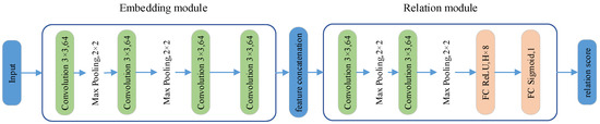
Figure 1.
The structure of relational networks.
The primary components consist of the embedding module and the relational module. The embedding module comprises four convolutional blocks along with two pooling layers, whereas the relational module consists of two convolutional blocks, two pooling layers, and two fully connected layers with eight and one neurons, respectively. Each convolutional block features a convolutional layer, a Batch Normalization layer, and a ReLU activation function.
2.4. Multi-Scale Coordinate Attention Mechanism
The attention mechanism enhances the model by generating corresponding weights for various extracted features, thereby making their characteristics more pronounced. Building upon coordinate attention [23], this paper introduces a multi-scale coordinate attention mechanism. This mechanism emphasizes relationships between different positions or coordinates in the input data, highlighting the significance of spatial information rather than merely considering relative feature relationships. By integrating a local scale branch, it enables cross-scale feature interaction and weight fusion. This approach processes spatial information in parallel across different scales, maintaining coordinate positioning accuracy while enhancing long-range dependency modeling capabilities. It is particularly effective for extracting and analyzing complex time–frequency features in mechanical fault diagnosis, offering a robust solution for high-precision diagnosis in scenarios characterized by small sample sizes and variable operating conditions. The structure of the multi-scale coordinate attention module is depicted in Figure 2.
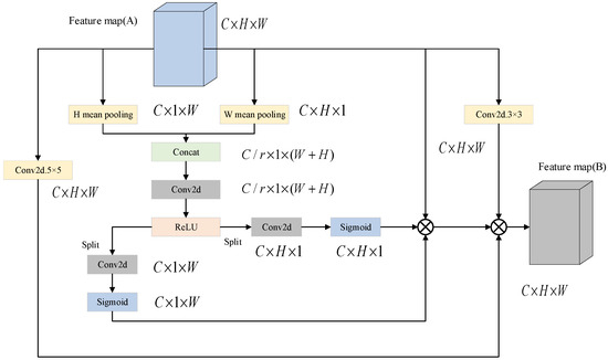
Figure 2.
Multi-scale coordinate attention module.
First, convolution operations are performed on the feature map using 3 × 3 and 5 × 5 convolution kernels to obtain feature maps A3×3 and A5×5. These feature maps will have shapes identical to the input feature map, with dimensions C × H × W.
Simultaneously, feature maps undergo average pooling operations in both horizontal and vertical orientations. In this phase, the output corresponding to the C-th channel in the height (H) direction can be represented as follows:
The output in the width (W) direction of the C-th channel can be expressed as
The concatenation of pooled feature maps results in a feature map sized C × (H + W). Following this, the features are combined and processed through nonlinear transformations using convolutional operations alongside ReLU activation functions, which produces a feature map with dimensions C/r × (H + W), where r denotes a scaling factor. Another convolutional operation is then performed, producing a feature map of size C × (H + W). This finalized fused feature map is split into two segments: one measuring C × H × 1 and the other measuring C × 1 × W.
Conduct convolution operations and utilize Sigmoid activation functions on the separated feature maps, generating attention weight maps sized C × H × 1 and C × 1× W. The values in these weight maps span from 0 to 1, reflecting the importance of different positions in the feature maps. By executing element-wise multiplication of the resulting attention weight maps with both the original input feature map and the feature maps modified by various convolution kernels, we produce feature maps that combine spatial attention information. These modified maps serve as the output feature maps B of the module.
The multi-scale coordinate attention module enhances the model’s feature representation and image analysis capabilities by extracting multi-scale features and applying attention mechanisms. This approach highlights crucial spatial information while suppressing irrelevant details in the input feature maps, ultimately providing higher-quality feature representations for subsequent network layers.
3. Small-Sample Fault Diagnosis Method
In order to tackle the issues related to complex feature extraction for rolling bearing faults and the limited availability of training samples, this study introduces a diagnosis approach for bearing faults that is founded on ALA-FMD and MSCA-RN. Figure 3 displays the flowchart that depicts this method.
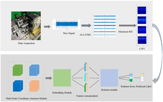
Figure 3.
Diagnostic method flowchart.
The original signal undergoes decomposition through FMD. To improve the precision of modal decomposition, ALA is utilized to fine-tune three parameters of FMD: the quantity of modes, the length of the filter, and the number of cutoff frequency bands. The minimum Residual Energy Index (REI) is used as the criterion for selecting the optimal modal components. The chosen optimal modal components are then converted from time-domain signals to two-dimensional time–frequency representations via CWT, which are later input into the MSCA-RN model for diagnosing faults.
3.1. ALA-FMD Method
The FMD method lacks the capability for parameter self-adaptation. Manual adjustments to parameters have been shown to exhibit poor stability and low efficiency. Specifically, an insufficient number of modes may result in the omission of critical fault information, while an excessive number of modes can introduce noise or redundant components [24]. Furthermore, an excessively short filter length (L) diminishes separation accuracy, whereas an overly long length increases the computational burden. Increasing the number of filters (K) enhances frequency resolution but simultaneously exacerbates computational complexity. If K is too small, important signal features may be overlooked, adversely affecting decomposition performance. Therefore, this paper employs ALA to optimize these three parameters, thereby improving both decomposition effectiveness and efficiency. The detailed steps of the ALA-optimized FMD are outlined as follows:
- (1)
- Initialize the population, set the maximum ALA iteration count to 100, and the population size N to 40. Since three parameters need to be optimized, the dimension size Dim is set to 3. This paper configures the mode within [3, 15], filter length within [64, 512], and the number of frequency band divisions within [2, 20], where ≥ .
- (2)
- To determine the fitness function, first break down the signal utilizing the FMD parameters associated with potential solutions. Next, calculate the envelope entropy value of the reconstructed signal, which will act as the fitness function needed to identify the best parameter combination. It is essential that both n and K are valid integers; if not, adjust them by truncating or rounding to the nearest acceptable value. Additionally, because L must meet linear phase requirements to avoid signal distortion, its coefficients should conform to either symmetric or antisymmetric rules, implying that L should be an even number.
- (3)
- Energy factor evaluation, calculate the magnitude of energy factors, determine whether to enter the exploration phase or the development phase.
- (4)
- During the exploration phase, there exists a 30% probability of expanding the search range by integrating the current optimal solution with random individuals through Brownian motion-based random perturbation. Conversely, there is a 70% probability of making periodic adjustments towards the optimal solution based on the current position.
- (5)
- During the development phase, there exists a 50% probability of performing a spiral search around the optimal solution for fine parameter tuning. Additionally, there is an equal probability of employing Lévy flights to facilitate local jumps, thereby preventing entrapment in local optima.
- (6)
- To evaluate and update, one must assess the fitness of new individuals. If these individuals demonstrate superiority over the current optimal solution, it is imperative to update the optimal solution accordingly.
- (7)
- If the total number of iterations has not been reached, continue to execute steps 2–6 until the desired iteration count is achieved, and then present the optimal combination of parameters.
3.2. MSCA-RN Fault Diagnosis Model
This paper proposes a multi-scale coordinate attention relational network model that integrates the advantages of relational networks for mining image features with the capabilities of a multi-scale coordinate attention mechanism to enhance features across varying scales, thereby facilitating the rapid diagnosis of bearing defects. By deeply integrating multi-scale feature engineering with relational networks, this model addresses the representational limitations of traditional attention mechanisms, which are often restricted to single-scale analysis. It offers a solution characterized by global structural localization, local detail enhancement, and multi-scale relationship measurement for bearing fault diagnosis. This approach is particularly effective in complex scenarios that involve small sample sizes and variable operating conditions.
3.3. Process Introduction
The fault diagnosis process of the multi-scale coordinate attention relational network is illustrated in Figure 4.
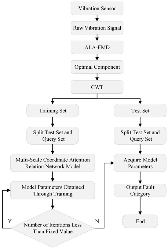
Figure 4.
Fault diagnosis model flowchart.
In the signal processing stage, the original vibration signals collected by vibration sensors are initially processed using the ALA-FMD. The optimal modal components are then selected based on the minimum residual index. Subsequently, these signals are transformed into two-dimensional time–frequency domain representations through continuous wavelet transform to elucidate fault characteristics. The processed time–frequency domain signals are categorized into training sets (comprising support sets and query sets) and test sets in accordance with the meta-learning strategy. Among them, the REI is used to measure the noise residue in the modal components, and the calculation formula is
In the equation, represents the original signal, and represents the reconstructed signal of the modal component. The smaller the REI value, the more effective energy is retained in the component, and less noise is present.
During the model training phase, the MSCA-RN employs a meta-learning episodic training strategy to enhance its generalization capability for few-shot faults through multi-task learning. Initially, the input time–frequency images undergo global position localization and local detail enhancement via the MSCA module. Subsequently, features are extracted through the convolutional blocks of the embedding module to obtain multi-scale fused features. The feature vectors from both the support and query sets are combined and fed into the relation module, where a nonlinear metric function generates relation scores within the [0–1] range. The optimization process utilizes Mean Squared Error (MSE) as the loss function, in conjunction with the Adam optimizer to dynamically adjust the learning rate. Through backpropagation, the MSCA parameters, convolutional kernel weights of the embedding module, and fully connected layer parameters of the relation module are updated, gradually reducing the discrepancy between predicted scores and ground truth labels. After iterative training, the model converges. This stage incorporates strategies of multi-scale feature enhancement along with meta-learning, allowing the model to comprehensively grasp both the overall structures and the specific details of fault features in scenarios with limited examples and varying operational conditions.
During the model testing phase, unlabeled bearing time–frequency diagrams are input into the trained network. The MSCA and embedding modules generate feature vectors, which are concatenated sequentially with the feature vectors of each fault category in the support set to form feature pairs. Subsequently, these pairs are processed through the relation module to compute similarity scores, aiding in the identification of fault types.
4. Dataset Validation
4.1. Dataset Introduction
To validate the noise reduction effect of ALA-FMD and the classification performance of the MSCA-RN model, this paper employs the Case Western Reserve University (CWRU) bearing dataset [25] to verify the proposed fault diagnosis method. The test rig is illustrated in Figure 5. The dataset was collected using acceleration sensors with SKF6205 (SKF Corporation, Gothenburg, Sweden) bearings at a sampling frequency of 12 kHz. It encompasses four load conditions, 0 hp, 1 hp, 2 hp, and 3 hp, with corresponding motor speeds set at 1797, 1772, 1750, and 1730 r/min, respectively. The four bearing conditions utilized in the experiment are classified as normal class (NC), inner ring Fault (IF), outer ring fault (OF), and rolling body fault (RF), with a fault diameter of 0.178 mm. The types of bearing fault data employed in the experiment are presented in Table 1.
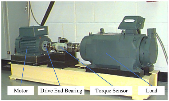
Figure 5.
Bearing test bench.

Table 1.
Bearing dataset fault types.
During the experiment, a sliding window sampling technique was employed on the original signal, with each sample comprising 8192 sampling points and a step size of 1200. The characteristic fault frequencies of the SKF6205 bearing are presented in Table 2.
Table 2.
SKF6205 fault characteristic frequency.
4.2. Original Signal Preprocessing
Initially, the noise reduction effect of ALA-FMD was verified. As illustrated in Figure 6, the time-domain diagrams of sound signals, corresponding to various faults at a 0 hp load, were processed using ALA-FMD for noise reduction.
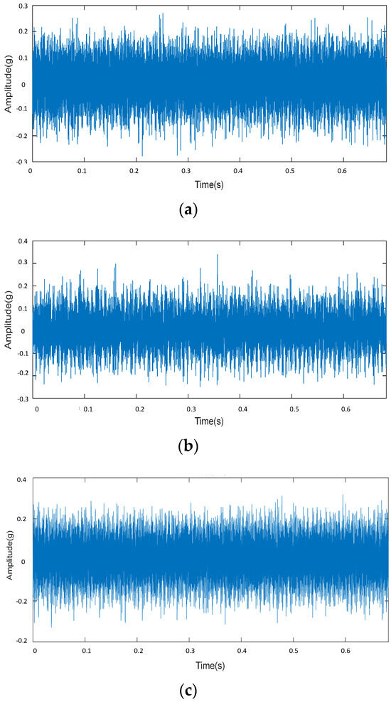
Figure 6.
Original signal of bearing dataset: (a) inner ring fault signal; (b) outer ring fault signal; (c) rolling body fault signal.
The optimal parameter set for FMD was determined using the ALA, aiming to minimize envelope entropy as the objective function. The outcomes of the optimization are visually examined throughout the process and compared against the results from the Crested Porcupine Optimizer (CPO), Particle Swarm Optimization (PSO), and Sparrow Search Algorithm (SSA). Figure 7 depicts the variation curve of envelope entropy, while Table 3 provides details on the optimal FMD configuration obtained through ALA optimization. The results indicate that the ALA reaches an envelope entropy of 0.58 and stabilizes after 20 iterations. In comparison, the PSO method achieves an envelope entropy of 1.02 after 74 iterations, showing a tendency to become trapped in local optima and demonstrating a slower optimization rate. Although PSO converges quickly in the early phases, it becomes vulnerable to local optima later on due to the convergence of particle velocities. The SSA initially prioritizes exploration, which limits its convergence speed. However, as the optimization process continues, the followers start to actively search, significantly improving convergence speed. Additionally, its capability to resist local optima exceeds that of the PSO method, yet its overall search effectiveness still lags behind that of the ALA method.
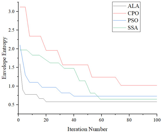
Figure 7.
Fitness function curve.
Table 3.
Optimal parameters for different fault types.
The data corresponding to different fault types were decomposed into signals using FMD, with the minimum REI employed as the selection criterion for optimal modal components. Figure 8 illustrates the REI values of each modal component for various bearing fault types.
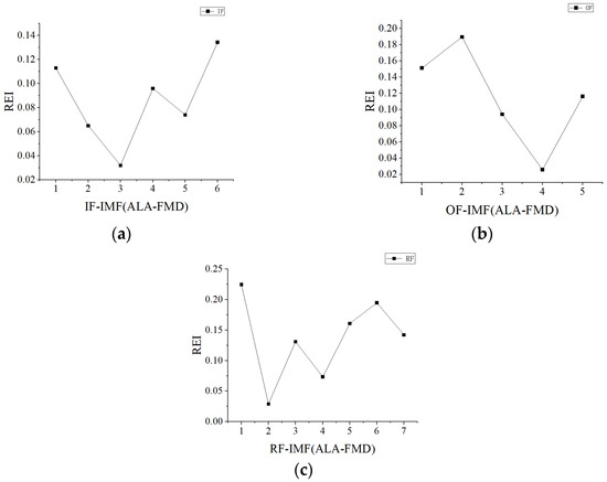
Figure 8.
REI values of different types of modal components: (a) inner ring modal component REI value; (b) outer ring modal component REI value; (c) rolling element modal component REI value.
According to the minimum REI selection principle, the third, fourth, and second modal components were selected for the bearing’s inner ring, outer ring, and rolling elements, respectively. The envelope spectra corresponding to the optimal components for various fault types are illustrated in Figure 9. From Figure 9a, the inner ring fault frequency and its sixth harmonic are clearly visible. From Figure 9b, the outer ring fault frequency and its ninth harmonic are distinctly observable. From Figure 9c, the rolling element fault frequency and its sixth harmonic are prominently evident.
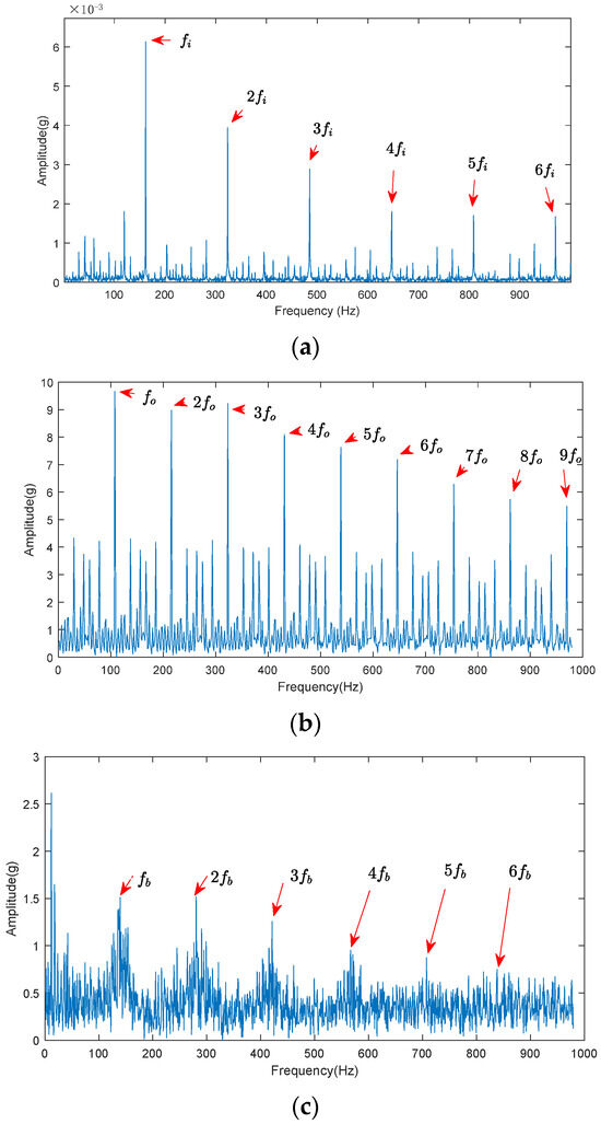
Figure 9.
Optimal component envelope spectrum for different faults: (a) inner race optimal component envelope spectrum; (b) outer race optimal component envelope spectrum; (c) rolling element optimal component envelope spectrum.
To assess the effectiveness of the method proposed in this paper, a comparison is made between the optimal component of the bearing inner race fault, selected through this approach, and the decomposition results obtained via fixed-parameter FMD, CPO-FMD, and adaptive VMD. For fixed-parameter FMD, the parameter settings are based on the research conducted by Y. Miao et al. [12], with the fixed FMD parameters set as follows: n = 4, L = 40, K = 5. Following the decomposition process for each method, the REI is utilized to identify the optimal component for conducting an envelope spectrum analysis. Figure 10 illustrates the optimal components and their corresponding envelope spectra derived from each method. As can be seen from Figure 10, although the fault frequency is visible, there are at most only four harmonics.
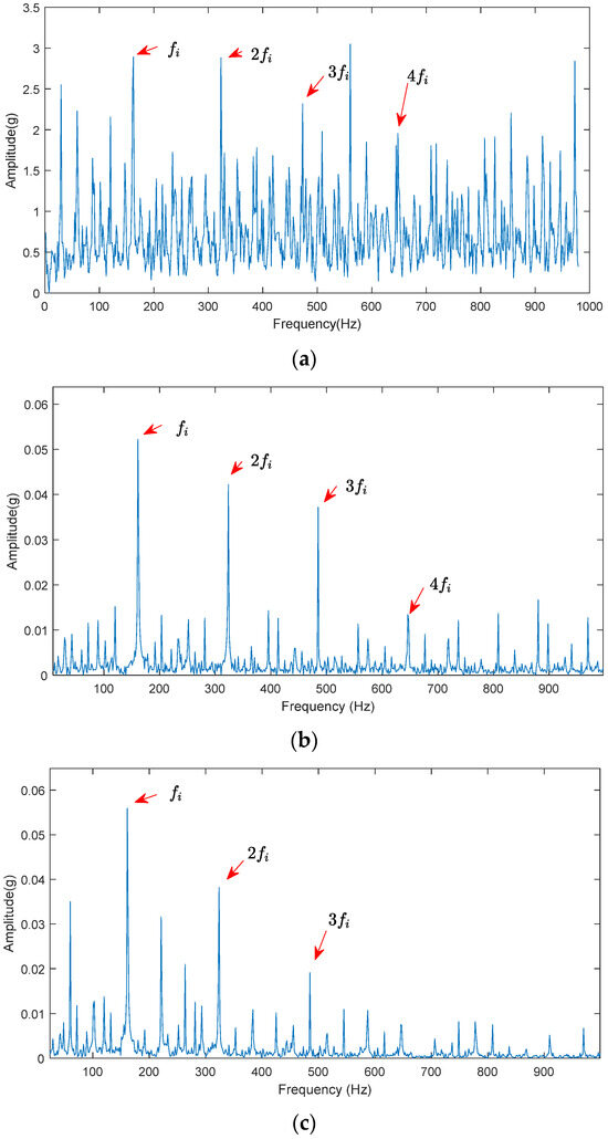
Figure 10.
Optimal component envelope spectrum for inner race fault decomposition using different methods: (a) optimal component envelope spectrum of fixed-parameter FMD for inner ring faults; (b) optimal component envelope spectrum of CPO-FMD for inner ring faults; (c) optimal component envelope spectrum of adaptive VMD for inner ring faults.
The analysis of Figure 9 and Figure 10 indicates that the proposed method effectively preserves fault information. This conclusion is substantiated by the envelope spectrum analysis, which demonstrates that ALA-FMD successfully extracts the fault characteristic frequency along with its multiple harmonic components. In contrast, the fixed-parameter FMD suffers from a lack of parameter adaptability, causing the effective information in the envelope spectrum to be obscured by noise. Furthermore, due to its limited optimization capabilities, CPO often converges to local optima, resulting in inferior decomposition performance when compared to ALA-FMD. Additionally, adaptive VMD exhibits limited effectiveness in extracting fault information in the presence of strong noise conditions.
4.3. Model Testing
The ideal elements acquired via ALA-FMD noise reduction decomposition underwent processing with CWT to create two-dimensional time–frequency representations. Figure 11 shows the time–frequency representations of the optimal elements post-CWT processing.
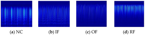
Figure 11.
Two-dimensional time–frequency diagrams of optimal components for different faults after CWT processing: (a) NC; (b) IF; (c) OF; (d) RF.
The dataset is split into training and testing subsets. In the training phase, each fault category, including normal bearings, consists of 20 samples, with five samples designated for the support set and 15 samples for the query set, thereby forming a four-way five-shot task. During the testing phase, 100 samples are selected for each fault category, with five samples allocated to the support set and the remaining samples to the query set. To assess the model’s generalization capability under varying operating conditions, three test sets are constructed based on different load conditions (0 hp, 1 hp, and 3 hp), which represent progressively greater deviations from the conditions of the training samples. The specific partitioning method is outlined in Table 4.
Table 4.
Test dataset.
The validity of the MSCA-RN was verified by inputting the obtained time–frequency maps into the MSCA-RN, RN, and coordinate attention relation network (CARN) for fault classification. The Adam optimizer’s initial learning rate was set to 0.001, and the model underwent 300 training iterations. To ensure the accuracy of the experimental results, the average of 10 test accuracies was used for evaluation. The confusion matrix for one instance of MSCA-RN classification is presented in Figure 12, while the average fault diagnosis accuracy is illustrated in Figure 13.
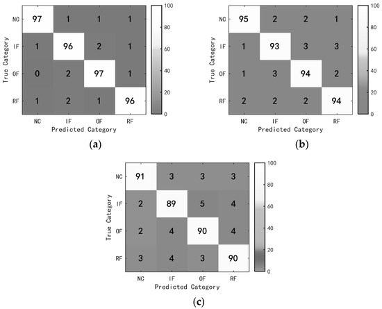
Figure 12.
Confusion matrix: (a) Test Set A; (b) Test Set B; (c) Test Set C.
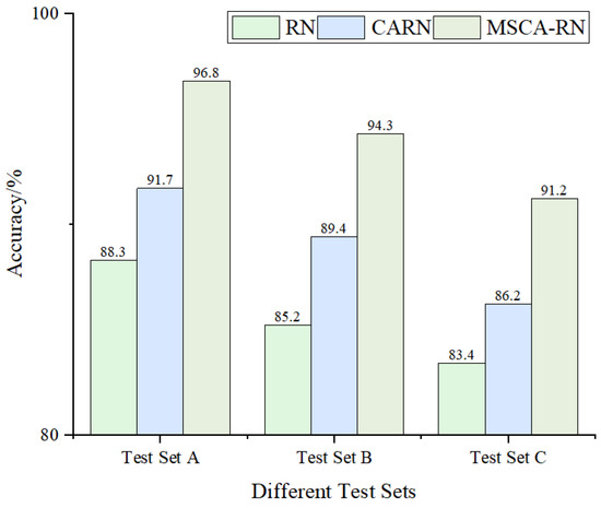
Figure 13.
Accuracy comparison of different models under varying loads.
As shown in Figure 12 and Figure 13, the model presented in this study demonstrates significantly higher overall accuracy when compared to both the RN and CARN models. In Test Set A, which functions under identical conditions to those of the training set, the MSCA-RN reaches a fault diagnosis accuracy of 96.8%. In contrast, the RN and CARN yield accuracies of 91.7% and 88.3%, respectively. In the context of variable operating conditions, MSCA-RN retains its superiority, achieving fault diagnosis accuracies of 94.3% for Test Set B and 91.2% for Test Set C, consistently outpacing both RN and CARN.
To validate the significant advantages of the proposed model in this paper, it was compared with current mainstream models, namely ResNet-34, CNN-GRU, and Transformer. The query set size for the MSCA-RN model was set to 5, and the obtained accuracy is illustrated in Figure 14. As demonstrated in Figure 14, the fault recognition accuracy of the method proposed in this paper surpasses that of the other models, with an average accuracy improvement of approximately 5% compared to ResNet-34, around 5.4% compared to CNN-GRU, and approximately 5.9% compared to Transformer.
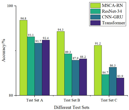
Figure 14.
Accuracy of different models.
To quantitatively evaluate the independent contributions of ALA-FMD and MSCA-RN, three control experiments were designed. The first experiment involved directly testing the untreated signal with RN for recognition. The second experiment involved inputting the signal processed with fixed-parameter FMD into RN for recognition. The third experiment involved inputting the signal processed with fixed-parameter FMD into MSCA-RN for recognition. The final accuracy comparison is presented in Table 5. As shown in Table 5, the ALA module improves recognition accuracy by approximately 4.9%, while the MSCA module enhances overall recognition accuracy by about 4.1%. This indicates that both the ALA module and the MSCA module hold significant value.
Table 5.
Ablation test accuracy.
5. Test Verification
5.1. Test Platform
In order to further assess the noise reduction capabilities of ALA-FMD and the performance of the MSCA-RN model in classification tasks, this study utilizes experimentally collected bearing vibration data to construct datasets for verification and analysis. The test rig is depicted in Figure 15. During the tests, various loads were applied to the rolling bearing corresponding to different rotational speeds: 0 hp, 1 hp, and 2 hp loads corresponded to main rotational speeds of 1800 r/min, 1780 r/min, and 1760 r/min, respectively. The YD-1A acceleration-type vibration sensor was employed for data acquisition with a sampling frequency of 25.6 kHz. The test bearing used was an SKF6215, with specific parameters listed in Table 6.
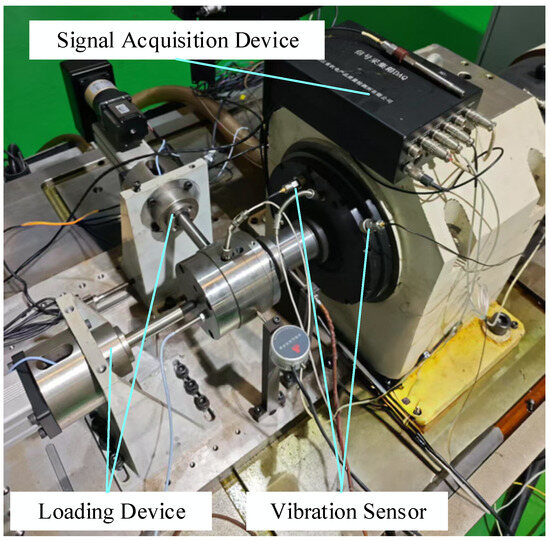
Figure 15.
SKF6215 bearing test rig.
Table 6.
SKF 6215 bearing parameters.
The fault frequency characteristics of the SKF6215 bearing at a rotational speed of 1800 r/min are presented in Table 7.
Table 7.
Fault characteristic frequency of SKF6215 bearing at 1800 r/min.
The damage condition of the faulty bearing part in the test is shown in Figure 16.
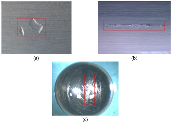
Figure 16.
Faulty bearing damage condition: (a) IF; (b) OF; (c) RF.
5.2. Data Preprocessing
The tested bearing types include four categories: inner race faults, outer race faults, rolling element faults, and normal bearings. After applying the ALA-FMD technique to process the vibration signals, the decomposition results of the original signals, along with the optimal modal components for each fault type, are presented in Figure 17.
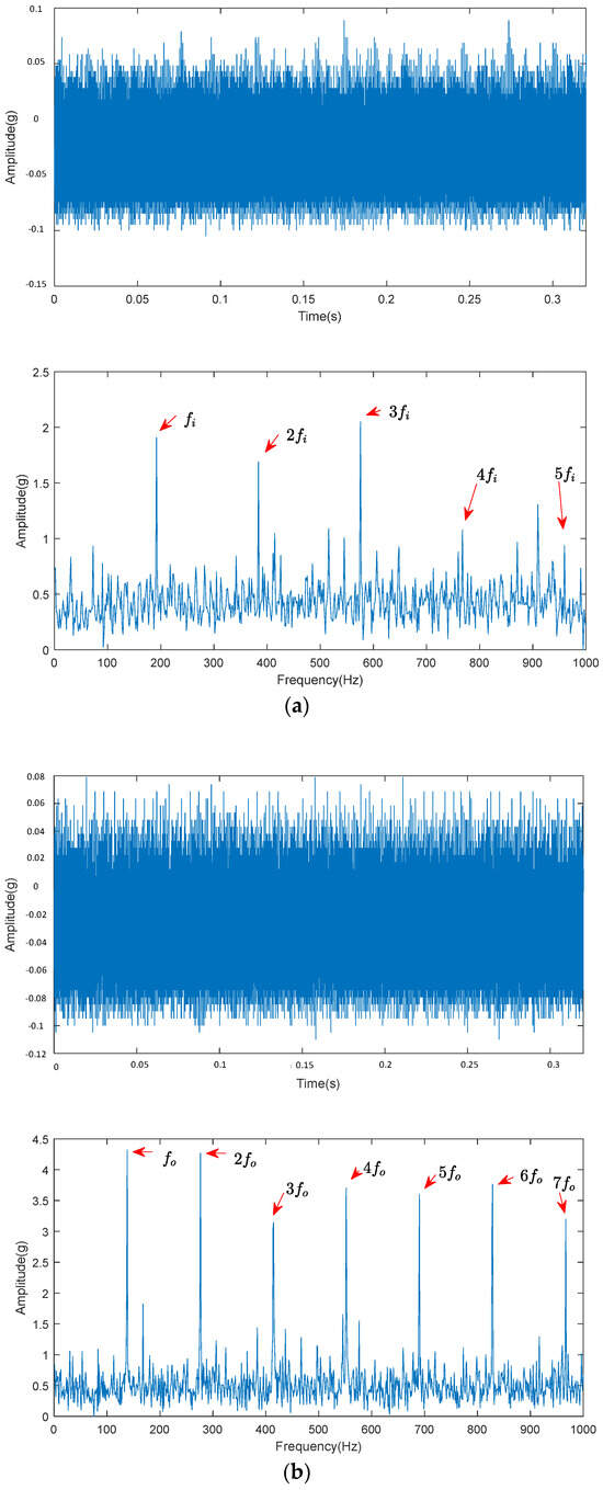
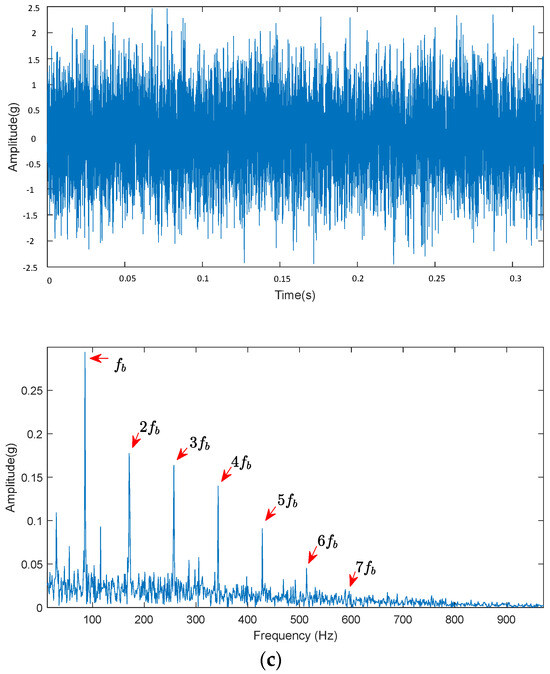
Figure 17.
Decomposition diagrams of ALA-FMD for different fault signals. (a) Original signal and optimal component envelope spectrum of SKF6215 inner ring fault. (b) Original signal and optimal component envelope spectrum of SKF6215 outer ring fault. (c) Original signal and optimal component envelope spectrum of SKF6215 rolling element fault.
Through the aforementioned methods, the ALA-FMD denoising was successfully accomplished. A comparative analysis presented in Table 8, which includes fixed-parameter FMD, CPO-FMD, and adaptive VMD, demonstrates that the proposed denoising method achieves significant improvements across all evaluated parameters.
Table 8.
Noise reduction effectiveness of different denoising methods.
To validate the feature extraction capability of ALA-FMD, it was compared with four contemporary deep feature extraction techniques: CNN-FE, VAE-FE, Transformer-FE, and DCNN-FE. The metrics used for comparison include SNR, REI, the inter-class to intra-class distance ratio (B/W Ratio), and the effective feature ratio (EF Ratio). The results of this comparison are presented in Table 9.
Table 9.
The feature extraction capabilities of different methods.
The SNR of ALA-FMD is 0.13 higher than that of DCNN-FE, while the REI is 32% lower. This indicates that the parameters optimized by ALA can decompose signals more accurately, preserving fault characteristics while effectively suppressing noise. Furthermore, the B/W Ratio and EF Ratio of ALA-FMD are 17.9% and 4.1% higher than those of DCNN-FE, respectively. This demonstrates that the extracted time–frequency features exhibit greater inter-class differences and more compact intra-class distributions in spatial terms. In deep learning models, Transformer-FE outperforms CNN-FE and VAE-FE due to the self-attention mechanism’s capability to capture long-range dependencies in non-stationary signals; however, it still falls short of the parameter-adaptive decomposition performance of ALA-FMD. Additionally, ALA-FMD feature extraction does not require training, providing significant advantages for industrial real-time diagnostics.
5.3. Sample Division and Model Validation Analysis
After converting the experimental data into time–frequency diagrams, we first conducted generalization performance tests under various loads. The test set comprised samples from different bearing faults subjected to varying loads, totaling 20 samples. This included five support set samples and 15 query set samples, thereby forming a four-way five-shot task. Similarly, the test set contained samples of different bearing faults under diverse loads, with 100 test samples per fault type (including bearing bearings), leading to a cumulative total of 400 test samples for each test set. Among these, five samples were designated as support set samples, while the remainder were classified as query set samples. The specific distribution is illustrated in Table 10.
Table 10.
Test data sample division.
In the four-way five-shot task, the model’s accuracy under varying loads is presented in Table 11. As illustrated in Table 11, the accuracy of the MSCA-RN model consistently surpasses that of both RN and CARN across different load conditions. Specifically, MSCA-RN achieves average accuracy improvements of 8.83% and 4.96% over RN and CARN, respectively, thereby demonstrating its superior generalization performance.
Table 11.
Model accuracy under different loads.
To further validate the variation in accuracy with different training sample sizes under the same load, we varied the number of samples during the training phase while maintaining 400 samples in the testing phase. This testing phase included 100 samples each for normal bearings, inner race faults, outer race faults, and rolling element faults. Building upon RN and CARN, this study compares MSCA-RN with both the channel attention-based SENet Relation Network (SERN) and the hybrid attention-based CBAM Relation Network (CBRN).
Initially, the fixed query set comprised 15 samples, while the support set was trained with 3, 5, and 10 samples, respectively. Figure 18 demonstrates the outcomes of the fault diagnosis.
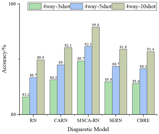
Figure 18.
Accuracy rates under varying numbers of support set samples.
As shown in Figure 18, the performance of each model enhances as the quantity of support set samples rises. The MSCA-RN model consistently achieves higher accuracy than other comparative models across different numbers of support set samples, outperforming the suboptimal model CARN by an average of about 5%, and improving the average accuracy by more than 6.8% compared to other models. This can be attributed to the ALA’s optimization of FMD, which enhances the representativeness of the extracted fault features. Furthermore, the multi-scale coordinate attention mechanism in MSCA-RN facilitates a more effective capture of multi-scale features in time–frequency diagrams, thereby strengthening the model’s fault identification capability.
Subsequently, with the number of support set samples set to 5, the total sample quantities were configured to 10, 20, and 40, respectively, with the diagnostic results illustrated in Figure 19.
Figure 19.
Accuracy rates under different total sample sizes.
As illustrated in Figure 19, the accuracy of all models improves further with an increase in the total sample size. The MSCA-RN model continues to maintain its leading position, with an average accuracy increase of over 7% compared to the baseline model RN, and an average accuracy increase of over 4.5% compared to other models. While other models show improved accuracy as well, their level of enhancement is comparatively less significant, underscoring the benefits of MSCA-RN in fault diagnosis, particularly when sample sizes are limited.
To further validate the generalization ability of the proposed method in this paper, data from the CWRU dataset, experimental data, and the SEU dataset were utilized. Data collected under the same operating conditions for different bearings within the datasets were compared and analyzed. The number of training samples remained at 20, and a four-way five-shot task was constructed. The accuracy results obtained from different datasets are shown in Table 12.
Table 12.
Accuracy of different datasets.
The experimental data achieved an accuracy rate of up to 94.6%, with accuracy rates for both the CWRU dataset and the SEU dataset exceeding 95.9%. Compared to other methods, the approach presented in this paper improved the average accuracy by at least 2%, demonstrating that the proposed model also exhibits excellent diagnostic performance across other datasets.
6. Conclusions
This paper introduces a new methodology for diagnosing bearing faults with few samples by combining ALA-FMD and MSCA-RN. This innovative solution merges biologically inspired global search strengths with local discriminative capabilities that are enhanced through multi-scale features, particularly in situations with limited data and varying operational conditions. ALA maintains a dynamic equilibrium between global exploration and local exploitation within the feature space by mimicking the behavior of lemmings, which can mitigate the overfitting issues of traditional meta-learning models under few-shot conditions to some extent. MSCA-RN employs the MSCA mechanism to capture cross-scale features in the time–frequency representations of bearing vibration signals, and combined with the nonlinear metric capabilities of RN, significantly improves the classification accuracy for similar fault categories. The integration of these two approaches accomplishes comprehensive enhancement from data feature enrichment to optimized search strategies, demonstrating effectiveness in overcoming the limitations of single models regarding feature representation and parameter optimization. Nonetheless, given that the assessments took place in controlled environments, whereas typical industrial conditions experience considerable fluctuations, upcoming studies will emphasize verifying the diagnostic capabilities of the model for various bearing faults across a range of industrial contexts.
Author Contributions
Conceptualization, H.W. and F.S.; methodology, H.W., F.S. and R.X.; software, H.W. and R.X.; validation, H.W., F.S. and R.X.; formal analysis, H.W. and F.S.; investigation, J.G. and C.L.; resources, J.G. and C.L.; data curation, H.W. and F.S.; writing—original draft preparation, F.S.; writing—review and editing, H.W. and R.X.; visualization, F.S. and R.X.; supervision, H.W.; project administration, H.W., R.X. and J.G.; funding acquisition, H.W. and R.X. All authors have read and agreed to the published version of the manuscript.
Funding
This work was supported by the Ningbo City Unveiled Project (2023T016). This work was supported by the Key Research and Development Program of Ningbo City and the “Unveiling the List and Appointing the Commander” Project (2023Z006).
Data Availability Statement
The data used to support the findings of this study are available from the corresponding author upon request. The test data in this article come from Bearing Luoyang Research Institute Co., Ltd.
Conflicts of Interest
Author Jinfang Gu was employed by the company Shanghai Tian An Bearing Co., Ltd. Author Chang Li was employed by the company Shandong Chaoyang Bearing Co., Ltd. The remaining authors declare that the research was conducted in the absence of any commercial or financial relationships that could be construed as a potential conflict of interest.
Abbreviations
The following abbreviations are used in this manuscript:
| ALA | Artificial Lemming Algorithm |
| FMD | Feature Mode Decomposition |
| MSCA | Multi-Scale Coordinate Attention |
| RN | Relation Network |
| CWRU | Case Western Reserve University |
| EMD | Empirical Mode Decomposition |
| IMF | Intrinsic Mode Functions |
| EEMD | Ensemble Empirical Mode Decomposition |
| CEEMD | Complementary EEMD |
| CEEMDAN | Complete Ensemble Empirical Mode Decomposition with Adaptive Noise |
| VMD | Variational Mode Decomposition |
| ISNN | Improved Siamese Neural Network |
| CWT | Continuous Wavelet Transform |
| FIR | Finite Impulse Response |
| CK | Correlation Kurtosis |
| CC | Correlation Coefficient |
| SNR | Signal-to-Noise Ratio |
| RMSE | Root Mean Square Error |
| MAE | Mean Square Error |
| REI | Residual Energy Index |
| MSE | Mean Squared Error |
| NC | Normal Class |
| IF | Inner-ring Fault |
| OF | Outer-ring Fault |
| RF | Rolling-body Fault |
| CPO | Crested Porcupine Optimizer |
| SERN | SENet Relation Network |
| CBRN | CBAM Relation Network |
References
- Yasenjiang, J.; Xiao, Y.; He, C.; Lv, L.; Wang, W. Fault Diagnosis of Bearings with Small Sample Size Using Improved Capsule Network and Siamese Neural Network. Sensors 2025, 25, 92. [Google Scholar] [CrossRef]
- Mian, T.; Choudhary, A.; Fatima, S. Vibration and Infrared Thermography Based Multiple Fault Diagnosis of Bearing Using Deep Learning. Nondestruct. Test. Eval. 2023, 38, 275–296. [Google Scholar] [CrossRef]
- Choudhary, A.; Goyal, D.; Letha, S.S. Infrared Thermography-Based Fault Diagnosis of Induction Motor Bearings Using Machine Learning. IEEE Sens. J. 2020, 21, 1727–1734. [Google Scholar] [CrossRef]
- Zhou, X.; Li, A.; Han, G. An Intelligent Multi-Local Model Bearing Fault Diagnosis Method Using Small Sample Fusion. Sensors 2023, 23, 7567. [Google Scholar] [CrossRef] [PubMed]
- Yang, Y.; Dong, X.J.; Peng, Z.K.; Zhang, W.M.; Meng, G. Vibration Signal Analysis Using Parameterized Time–Frequency Method for Features Extraction of Varying-Speed Rotary Machinery. J. Sound Vib. 2015, 335, 350–366. [Google Scholar] [CrossRef]
- Wu, Z.; Huang, N.E. Ensemble Empirical Mode Decomposition: A Noise-assisted Data Analysis Method. Adv. Adapt. Data Anal. 2009, 1, 1–41. [Google Scholar] [CrossRef]
- Zheng, J.; Cheng, J.; Yang, Y. Partly Ensemble Local Characteristic-Scale Decomposition: A New Noise Assisted Data Analysis Method. Acta Electron. Sin. 2013, 41, 1030–1035. [Google Scholar] [CrossRef]
- Yeh, J.R.; Shieh, J.S.; Huang, N.E. Complementary Ensemble Empirical Mode Decomposition: A Novel Noise Enhanced Data Analysis Method. Adv. Adapt. Data Anal. 2010, 2, 135–156. [Google Scholar] [CrossRef]
- Torres, M.E.; Colominas, M.A.; Schlotthauer, G.; Flandrin, P. A Complete Ensemble Empirical Mode Decomposition with Adaptive Noise. In Proceedings of the IEEE International Conference on Acoustics, Speech and Signal Processing, Prague, Czech Republic, 22–27 May 2011; pp. 4144–4147. [Google Scholar] [CrossRef]
- Dragomiretskiy, K.; Zosso, D. Variational Mode Decomposition. IEEE Trans. Signal Process. 2014, 62, 531–544. [Google Scholar] [CrossRef]
- Li, Y.; Cheng, G.; Liu, C. Research on Bearing Fault Diagnosis Based on Spectrum Characteristics Under Strong Noise Interference. Measurement 2021, 169, 108509. [Google Scholar] [CrossRef]
- Miao, Y.; Zhang, B.; Li, C.; Lin, J. Feature Mode Decomposition: New Decomposition Theory for Rotating Machinery Fault Diagnosis. IEEE Trans. Ind. Electron. 2023, 70, 1949–1960. [Google Scholar] [CrossRef]
- Xu, S.; Zhang, C. Compound Fault Diagnosis Method for Rolling Bearings Based on Feature Mode Decomposition Optimized by Whale Optimization Algorithm. J. Mech. Electr. Eng. 2025, 1–11. Available online: https://link.cnki.net/urlid/33.1088.TH.20250408.1047.006 (accessed on 29 June 2025).
- Shi, Y.; Huang, Y.; Wang, F.; Shi, J.; Zhang, J. Fault Diagnosis of Rolling Bearing under strong background noise based on POFMD. J. Vib. Shock 2024, 43, 107–115. [Google Scholar]
- Liu, Y.; Cai, H.; Li, W.; Zhao, S.; Liu, C. Research on Deep Convolutional Generative Adversarial Networks Diagnosis Method of Bearing Fault Under Small Sample Condition. J. Vib. Meas. Diagn. 2023, 43, 817–823, 836. [Google Scholar]
- Wu, G.; Liu, X.; Bi, H.; Fan, W.; Tu, L. Review of Personalized Recommendation Research Based on Meta-Learning. Comput. Eng. Sci. 2024, 46, 338–352. [Google Scholar]
- Guo, N.; Di, K.; Liu, H.; Wang, Y.; Qiao, J. A Metric-Based Meta-Learning Approach Combined Attention Mechanism and Ensemble Learning for Few-Shot Learning. Displays 2021, 70, 102065. [Google Scholar] [CrossRef]
- Zhao, X.; Ma, M.; Shao, F. Bearing Fault Diagnosis Method Based on Improved Siamese Neural Network with Small Sample. J. Cloud Comput. 2022, 11, 79. [Google Scholar] [CrossRef]
- Wu, J.; Zhao, Z.; Sun, C.; Yan, R.; Chen, X. Few-Shot Transfer Learning for Intelligent Fault Diagnosis of Machine. Measurement 2020, 166, 108202. [Google Scholar] [CrossRef]
- Guo, M.; Chen, P.; Zhou, C. Few-Shot Bearing Fault Diagnosis Based on Coordinate Attention Relation Network. J. Sichuan Univ. (Nat. Sci. Ed.) 2024, 61, 047001. [Google Scholar] [CrossRef]
- Liu, X.; Chen, Z.; Hu, D.; Zong, L. A Novel Framework Based on Complementary Views for Fault Diagnosis with Cross-Attention Mechanisms. Electronics 2025, 14, 886. [Google Scholar] [CrossRef]
- Xiao, Y.; Cui, H.; Khurma, R.A.; Castillo, P.A. Artificial Lemming Algorithm: A Novel Bionic Meta-Heuristic Technique for Solving Real-World Engineering Optimization Problems. Artif. Intell. Rev. 2025, 58, 84. [Google Scholar] [CrossRef]
- Hou, Q.; Zhou, D.; Feng, J. Coordinate Attention for Efficient Mobile Network Design. In Proceedings of the IEEE/CVF Conference on Computer Vision and Pattern Recognition, Nashville, TN, USA, 20–25 June 2021; pp. 13713–13722. [Google Scholar] [CrossRef]
- Wang, X.; Li, C.; Tian, H.; Xiong, X. A Step-by-Step Parameter-Adaptive FMD Method and Its Application in Fault Diagnosis. Meas. Sci. Technol. 2024, 35, 046109. [Google Scholar] [CrossRef]
- Smith, W.A.; Randall, R.B. Rolling Element Bearing Diagnostics Using the Case Western Reserve University Data: A Benchmark Study. Mech. Syst. Signal Process. 2015, 64, 100–131. [Google Scholar] [CrossRef]
Disclaimer/Publisher’s Note: The statements, opinions and data contained in all publications are solely those of the individual author(s) and contributor(s) and not of MDPI and/or the editor(s). MDPI and/or the editor(s) disclaim responsibility for any injury to people or property resulting from any ideas, methods, instructions or products referred to in the content. |
© 2025 by the authors. Licensee MDPI, Basel, Switzerland. This article is an open access article distributed under the terms and conditions of the Creative Commons Attribution (CC BY) license (https://creativecommons.org/licenses/by/4.0/).