Optimized FPGA Architecture for CNN-Driven Subsurface Geotechnical Defect Detection

Abstract

Convolutional neural networks (CNNs) are widely used in geotechnical engineering. Real-time detection in complex geological environments, combined with the strict power constraints of embedded devices, makes Field-Programmable Gate Array (FPGA) platforms ideal for accelerating CNNs. Conventional parallelization strategies in FPGA-based accelerators often result in imbalanced resource utilization and computational inefficiency due to varying kernel sizes. To address this issue, we propose a customized heterogeneous hybrid parallel strategy and refine the bit-splitting approach for Digital Signal Processor (DSP) resources, improving timing performance and reducing Look-Up Table (LUT) consumption. Using this strategy, we deploy the lightweight YOLOv5n network on an FPGA platform, creating a high-speed, low-power subsurface geotechnical defect-detection system. A layer-wise quantization strategy reduces the model size with negligible mean average precision (mAP) loss. Operating at 300 MHz, the system reduces LUT usage by 33%, achieves a peak throughput of 328.25 GOPs in convolutional layers, and an overall throughput of 157.04 GOPs, with a power consumption of 9.4 W and energy efficiency of 16.7 GOPs/W. This implementation demonstrates more balanced performance improvements than existing solutions.

1. Introduction

In recent years, deep learning techniques have increasingly been applied in geotechnical engineering, offering a new approach for detecting subsurface structural safety hazards. CNNs have shown superior performance over traditional ground-penetrating radar (GPR) interpretation techniques in applications such as tunnel-lining crack identification [1,2], slope rock-mass loosening zone analysis [3,4], and underground pipeline-corrosion detection [5]. Conventional methods rely on manual interpretation of radar waveforms, leading to inefficiency and subjectivity. In contrast, CNNs allow end-to-end feature learning, directly extracting multi-scale defect representations from raw radar echo images. However, real-time detection requirements in complex geological environments, combined with the stringent power constraints of embedded devices, present dual challenges for designing lightweight network architectures and improving hardware acceleration efficiency.

Among CNN architectures, the YOLO series algorithms have garnered widespread attention since their inception, due to their exceptional detection speed and highly reliable accuracy [6,7]. In recent years, the YOLO series models have continuously iterated and upgraded, with versions such as YOLOv8 and YOLOv9 being released, introducing dynamic label assignment, more complex feature fusion modules, and expanded task support, further improving detection performance in general scenarios. YOLOv12 integrates attention mechanisms into the YOLO framework and further enhances accuracy and speed through innovations such as R-ELAN, FlashAttention, and regional attention [8]. However, in the specific field of underground geotechnical defect detection, model selection must prioritize balancing accuracy, efficiency, and hardware compatibility. On one hand, defect targets in geophysical radar images, such as cracks and loose bodies, have relatively fixed shapes, and the background noise is complex. Over-parameterized models can lead to overfitting and computational redundancy. On the other hand, the limited resources of embedded platforms require models to have extremely lightweight characteristics. In this context, YOLOv5n—a lightweight variant of the series—becomes the ideal choice for efficient inference on embedded platforms for underground geotechnical defect detection. YOLOv5n achieves an optimal balance between model compactness and detection accuracy through its simplified CSPNet backbone and cross-stage feature fusion strategy [9,10]. Its adaptive anchor-box calculation module [11] and Mosaic data augmentation technique [12] provide significant advantages in underground geotechnical defect detection. Additionally, YOLOv5n supports progressive quantization from FP32 to INT8, compressing the size of the quantized model to 24.3% of its original size [13].

While YOLOv5n excel in image feature representation, their high-dimensional parameter spaces and computational demands [14] impose significant challenges on hardware platforms. CPUs typically deliver only 10–100 GFLOPS of computational throughput under standard workloads [15], constrained by the serial execution paradigm of von Neumann architectures, which results in suboptimal energy efficiency. Although GPUs achieve TFLOPS-level computational power via massively parallel streaming multiprocessor arrays, their high power consumption and physical size hinder deployment in embedded systems. In contrast, FPGAs leverage hardware-level parallelism, dynamically reconfigurable configurable logic blocks (CLBs), and customized dataflow engines to optimize convolutional operations, achieving Pareto-optimal performance–power tradeoffs for edge inference tasks [16,17].

Previous researchers have made effective explorations in YOLO network accelerators on FPGA platforms. Shafiei et al. designed a scalable core supporting 1 × 1, 3 × 3, and 5 × 5 convolutional kernels, utilizing 13-bit floating-point computation to implement YOLOv4-tiny on FPGA, achieving a 62% reduction in resource utilization and a 43% decrease in latency compared to baseline implementations [18]. Yan et al. proposed a hardware-friendly full-network 4-bit quantization algorithm and an FPGA-based YOLO accelerator design, achieving both high inference accuracy and throughput [19]. Kim et al. designed a spatially grouped feature map buffer that continuously supplies data streams to processing units, enabling the implementation of an efficient hardware accelerator design for YOLOv3-tiny [20].

In the field of defect detection, Guo Runyuan proposed a welding defect-detection method based on Generative Adversarial Networks combined with transfer learning, improving defect-detection accuracy [21]. David Jie deployed YOLOv2 on the Zynq series FPGA to detect surface defects on aluminum plates [22]. VC Johnson used the Haar cascade classifier and Local Binary Pattern (LBP) classifier algorithm to design an FPGA hardware accelerator for surface defect detection of metal fixtures [23].

Huang et al. proposed a 14 × 14 DSP matrix acceleration strategy to maximize FPGA parallelism and enhance processing unit utilization [17]. Meanwhile, Zhang et al. introduced a generalized DSP array design to accelerate convolutions of varying sizes [15]. However, these generalized designs are inefficient, due to the dimensional variability of convolution operations. Specifically, 3 × 3 convolutions show quadratic growth in computational complexity with input/output channel counts, while 1 × 1 convolutions scale linearly. Uniform parallelization strategies increase resource consumption and imbalance computational efficiency.

This work addresses these challenges through the following contributions:

(1)

We design a heterogeneous parallel architecture with dedicated DSP arrays optimized for the distinct operational characteristics of the 1 × 1 and 3 × 3 kernels in YOLOv5n, reducing resource redundancy caused by uniform parallelization.

(2)

We have improved the mainstream bit-partitioning strategy for DSP resources. We optimized the timing and reduced LUT resource consumption while ensuring unchanged DSP resource consumption and computational efficiency.

(3)

In dataflow design, we employ a row-buffered streaming architecture to form a multi-row data pool for sliding window operations, increasing the utilization of on-chip block RAM (BRAM) and reducing redundant data reloading.

2. Algorithmic Foundation

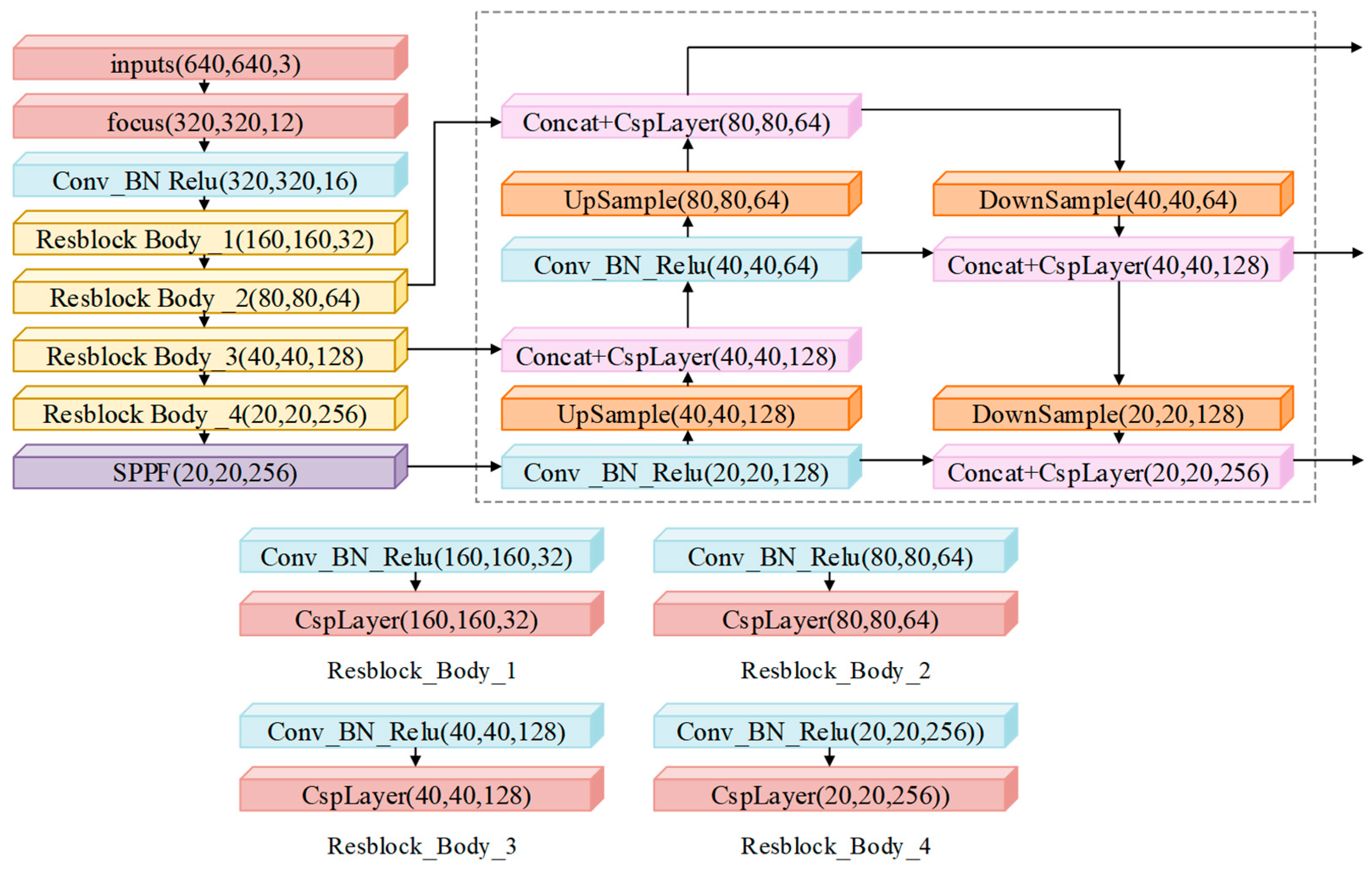
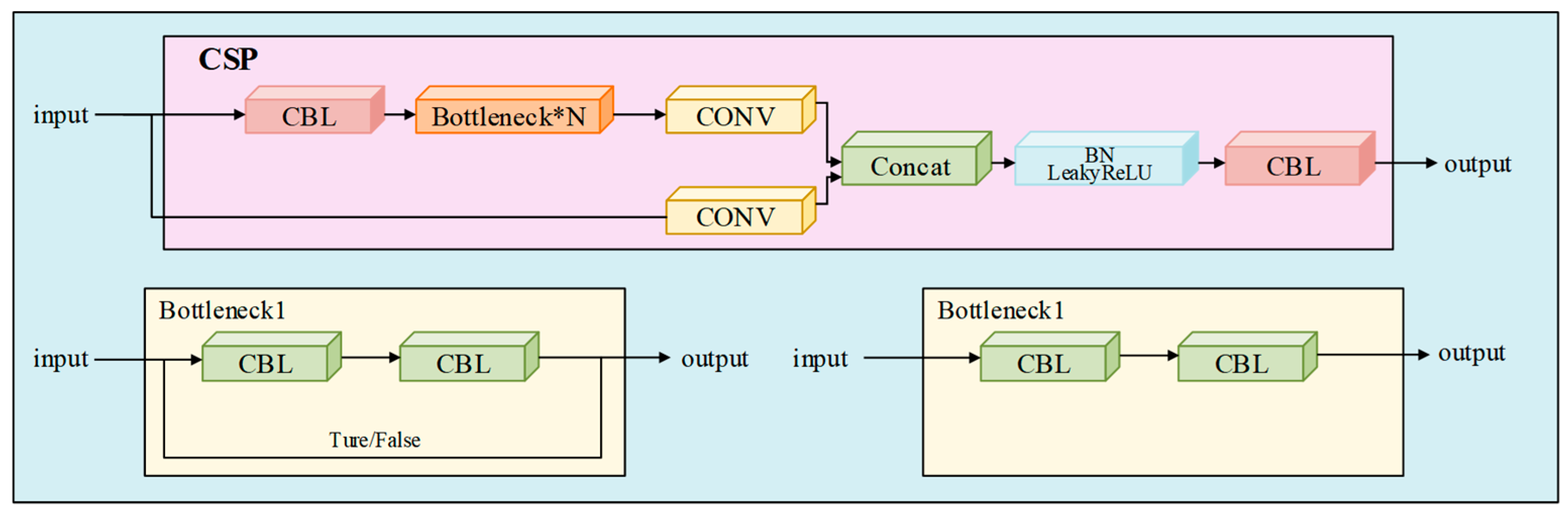
2.1. Architecture and Operational Principles of YOLOv5n

As shown in Figure 1, YOLOv5n adopts an efficient detection framework [24]. First, the Backbone performs rapid down sampling on the input image through convolutional blocks and uses the SPPF module to expand the receptive field. It then outputs feature maps at three scales: 80 × 80, 40 × 40, and 20 × 20. These feature maps are processed by the Neck for effective multi-scale feature aggregation. Finally, Non-Maximum Suppression (NMS) is applied to remove redundant detection boxes, outputting the final detection results.

However, with increasing network depth, two fundamental issues arise: computational redundancy [25] and gradient attenuation. YOLOv5n addresses these challenges by adopting CSPDarknet53 as its backbone network. The core innovation of CSPNet lies in partitioning feature information into two paths: a main path for refined processing and a bypass path that preserves raw information, which merge at key nodes. This design retains the representational capacity of deep networks while significantly reducing computational costs.

As shown in Figure 2, the input feature map (dimensions H × W × C) is evenly split into two streams. The main path processes C/2 channels through a residual block subnet involving sequential convolution, batch normalization, and activation functions for feature refinement. The bypass path directly transmits the remaining C/2 channels, circumventing the subnet. The outputs of both paths are concatenated along the channel dimension to reconstruct an H × W × C feature map. The concatenated features undergo 1 × 1 convolution for channel compression and integrate skip connections to form the final output. For a traditional 3 × 3 convolution, C × C × 3 × 3 Multiply Accumulate (MAC) operations are required. In the CSP module, the main path processes only C/2 channels, reducing MAC operations to (C/2) × (C/2) × 3 × 3—halving the computational load. Additionally, the bypass path acts as a “gradient highway,” allowing gradients to bypass deep subnets during backpropagation and alleviating vanishing gradient issues.

Moreover, YOLOv5n further optimizes the Spatial Pyramid Pooling (SPP) module into Spatial Pyramid Pooling Fast (SPPF), replacing parallel pooling layers with serially stacked max-pooling layers. This modification effectively reduces computational burden while retaining multi-scale feature fusion capabilities [26]. After the backbone extracts deep features, the SPPF module rapidly integrates multi-scale contextual information. The neck architecture then constructs a bidirectional feature pyramid through upsampling and cross-layer connections: high-semantic deep features propagate top–down to refine localization accuracy, while high-resolution shallow features flow bottom–up to enrich detail perception in deeper layers [27]. Finally, the head layer outputs three feature maps at 80 × 80, 40 × 40, and 20 × 20 resolutions, specialized for detecting small, medium, and large targets.

2.2. The 8-Bit Quantization Strategy

In edge deployment of deep learning models, 8-bit quantization technology significantly optimizes computational efficiency and storage overhead by reducing data precision [28,29]. To address the architectural characteristics of YOLOv5n, this scheme adopts a hybrid strategy combining symmetric quantization and layer-wise quantization. Given the symmetric distribution of weights, zero-centered symmetric quantization is employed to eliminate zero-point offset calculations. Compared to per-channel quantization—which requires maintaining independent scale and zero-point parameters for each convolutional kernel channel—layer-wise quantization reduces the quantization parameters to a single global set per layer, thereby substantially lowering computational complexity.

$$q_1=round({\displaystyle \frac{r_1}{s_1}}-z_1)$$

(1)

$$q_2=round({\displaystyle \frac{r_2}{s_2}})$$

(2)

s1 and s2 denote the scale factors for activations and weights, respectively, and z1 represents the activation zero-point offset. In symmetric quantization, the zero-point offset is used to precisely map the floating-point zero to the integer domain, addressing the asymmetry in data distribution and eliminating systematic errors during the quantization process. By fusing batch normalization layers with convolution operations, the quantized output feature map is simplified as

$$q_3={\displaystyle \frac{s_1\cdot s_2}{s_3}}\cdot q_1\otimes q_2\left[1\right]-({\displaystyle \frac{s_1\cdot s_2}{s_3}}\cdot z_1\cdot q_2+z_3)\left[2\right]+{\displaystyle \frac{bias}{s_3}}\left[3\right]$$

(3)

The parameter s3 represents the output scale factor, which rescales the integer convolution results back to the numerical range aligned with the floating-point output values, ensuring numerical equivalence during the quantization process. The parameter z3 represents the output zero-point offset, and is included in the constant term. The multiplication operator in formula items [1] denotes the quantized integer convolution operation. Bias represents the bias quantization calibration after the fusion of the convolutional layer and the Batch Normalization (BN) layer, which is used to correct the accumulated errors from the fusion of BN and quantization. Formula items [2] and [3] are precomputed as constants and embedded into lookup tables, eliminating real-time scaling and offset adjustment overhead. This design substantially reduces hardware logic complexity while mitigating detection accuracy degradation caused by cumulative quantization noise. The 8-bit quantization scheme reduces storage requirements for weights and activations to 25% of the floating-point baseline while maintaining model accuracy.

3. Accelerator Architecture

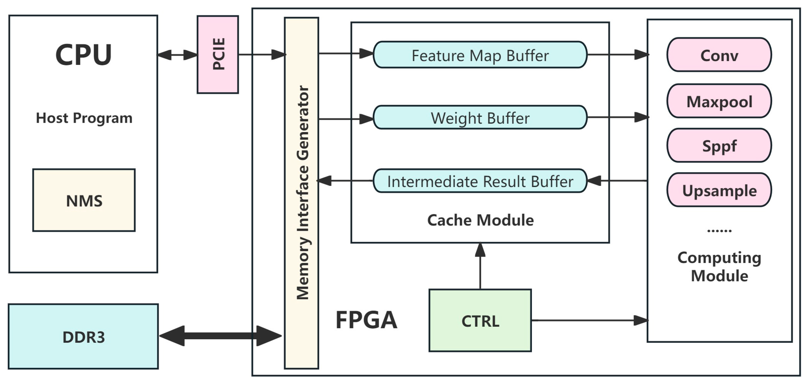
3.1. Overall Hardware Architecture

The top-level architecture of the proposed YOLO accelerator is shown in Figure 3.

Specifically, raw image data and weights are transferred from the CPU to the FPGA’s external memory via PCIe, while relevant scheduling instructions are loaded into the FPGA’s on-chip RAM. To reduce energy consumption caused by DDR3 data transfers, an AXI Direct Memory Access (AXI_DMA) interface is employed to facilitate efficient interaction between external memory and on-chip memory, where feature maps and weights are stored in on-chip BRAMs. The cache module and computing units interact through the FPGA’s internal control logic to perform rapid operations such as convolution, SPPF, and upsampling. Upon power-up, the FPGA first decodes the instructions. Subsequently, under the instruction scheduling, it initiates layer-by-layer computation, with intermediate results being returned to DDR3 after each layer. After completing the final convolutional layer, the results are transmitted back to the CPU for post-processing tasks, including Non-Maximum Suppression (NMS) and visualization.

3.2. Dataflow Buffer Design

In hardware architectures designed to accelerate convolutional neural networks, optimizing dataflow management is critical for overcoming memory bottlenecks. This study proposes a sliding window generation mechanism based on multi-line buffering, achieving spatiotemporal reuse of feature map data through a circular queue structure with line buffers. As shown in Figure 4, the input feature map is partitioned into row-based storage units using five independent RAM modules to construct a ring buffer queue. Each RAM module’s depth aligns with the input feature map width, storing consecutive rows vertically in sequence. For 3 × 3 convolution operations, the sliding window updates dynamically: initially, the first three rows are fetched from RAM1 to RAM3 to form the initial convolution window. After processing, the second and third rows are retained, while the fourth row is fetched from RAM4 and RAM1 is updated with the sixth-row data. This row replacement mechanism ensures seamless data transitions and eliminates redundant data fetches in traditional sliding window methods.

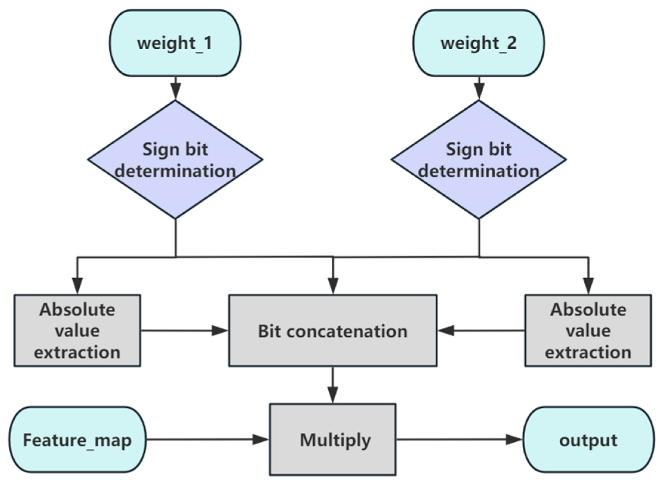
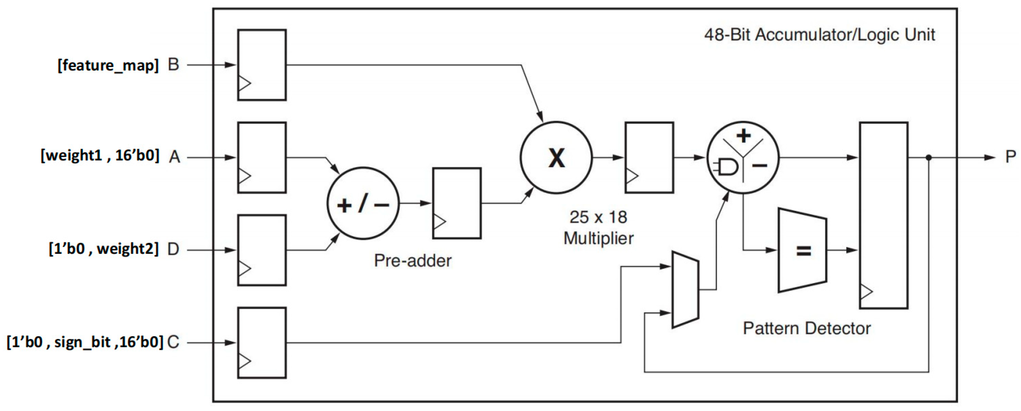
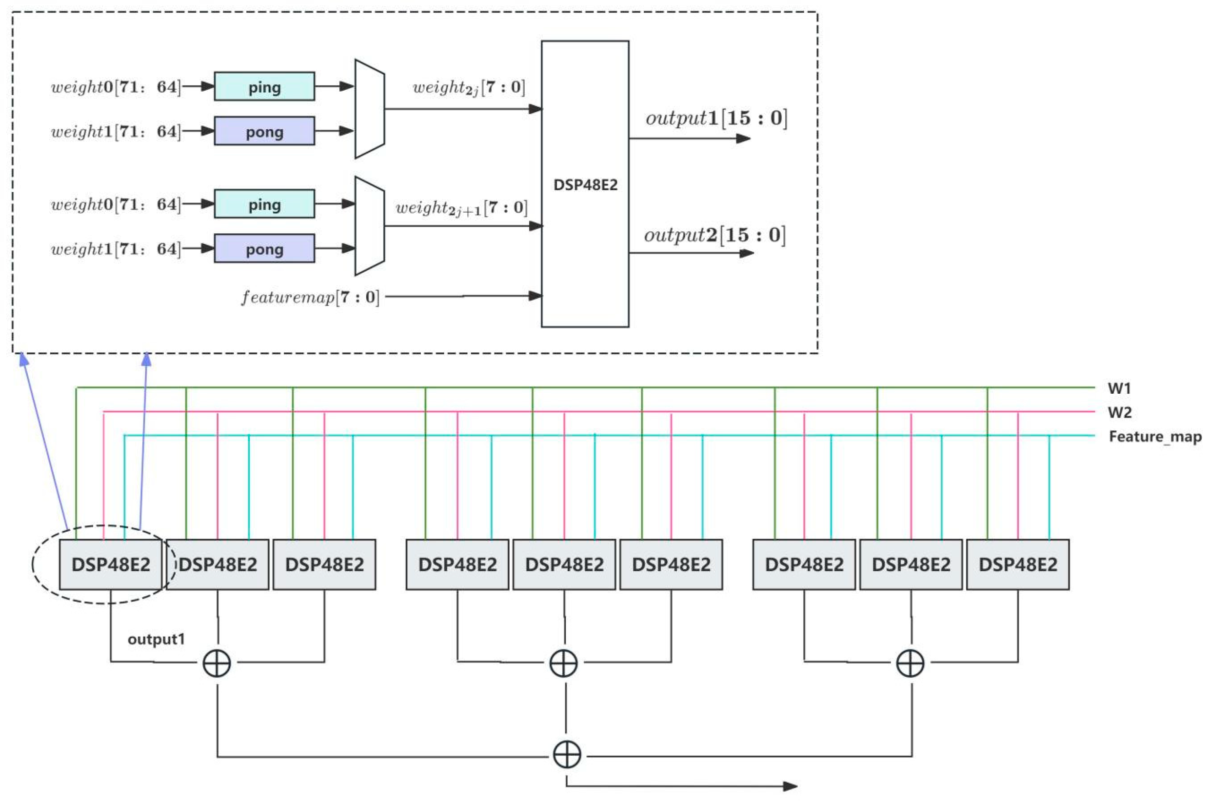
3.3. High Bit-Width Partitioning Strategy for DSPs

When designing convolutional accelerators on resource-constrained platforms, efficient reuse of DSP units is critical to overcoming hardware bottlenecks. Leveraging the architectural features of Xilinx DSP48E1, we adopt an improved DSP bit-width partitioning scheme that achieves lower LUT resource consumption and optimized timing compared to mainstream DSP design methods under equivalent DSP resource utilization.

Mainstream DSP bit-width partitioning approaches enable superlinear resource reuse by reconstructing data mapping relationships at multiplier input ports. As illustrated in Figure 5, this method divides the 25-bit port into two independent 8-bit weight interfaces after sign-bit determination: the lower byte [7:0] carries weight parameters for output channel index 2j, while the adjacent higher byte [23:16] stores weights for index 2j + 1, with the remaining bits padded with zeros. This bit-width reconfiguration strategy allows a single DSP unit to perform two independent 8-bit fixed-point multiplication operations within the same clock cycle, theoretically reducing DSP resource requirements by 50%.

However, traditional methods rely on external logic circuits to handle sign-bit determination, data concatenation, and result adjustment for multi-task parallel computation, which incur significant LUT resource overheasd and introduce latency. To address this, we propose an improved high-bit-width partitioning scheme for DSP48E1. As shown in Figure 6, DSP48E1 integrates not only a multiplier, but also a pre-adder and an accumulator. The pre-adder eliminates sign-bit determination and enables seamless signed-number bit concatenation. When the second weight is negative, this method introduces computational deviation. To compensate, the accumulator injects a sign-based correction term, thereby eliminating the resource consumption associated with result adjustment in the original scheme.

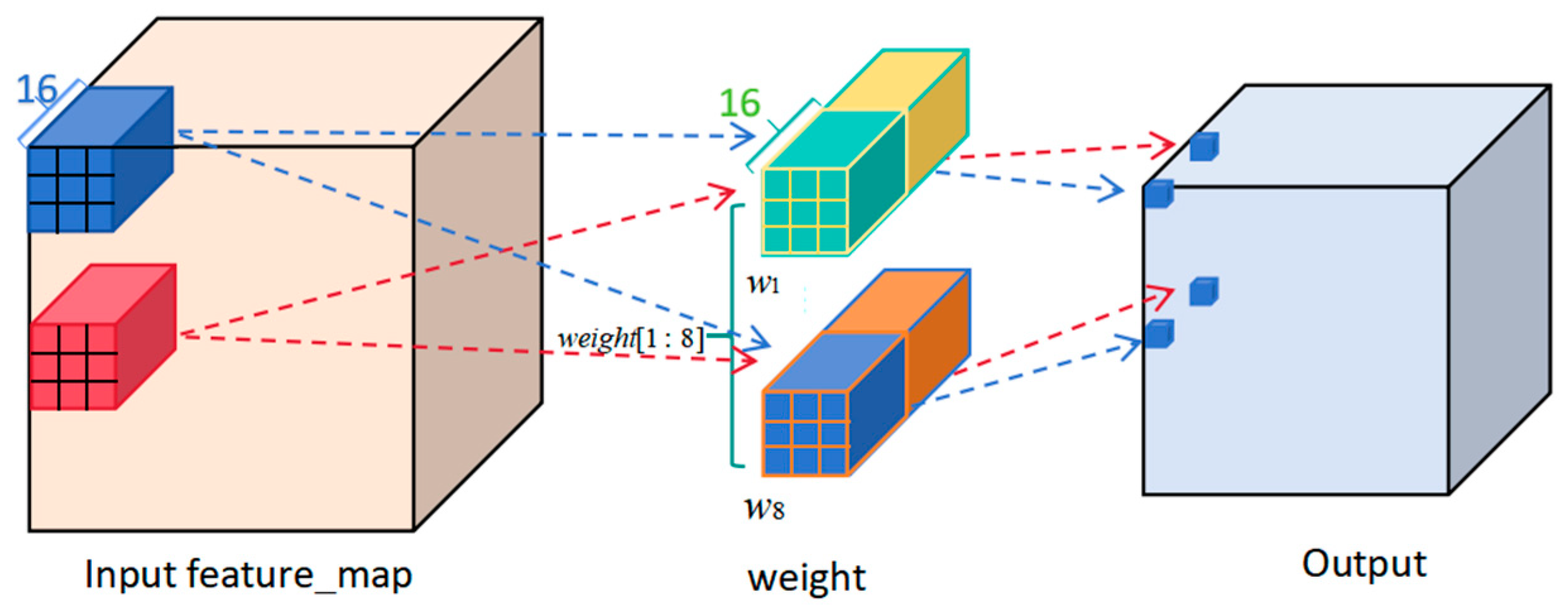
3.4. Convolutional Layer Hybrid-Acceleration Strategy

In the design of deep learning accelerators for edge computing, deploying CNNs on FPGA-based hardware platforms faces the dual challenges of computational efficiency and hardware resource limitations. As seen from (4), the computational intensity of a 3 × 3 convolution is 9 times that of a 1 × 1 convolution.

$${\displaystyle \frac{{MAC}_{3\times 3}}{{MAC}_{1\times 1}}}={\displaystyle \frac{Cin\times 3\times 3\times H_{OUT}\times W_{OUT}}{Cin\times 1\times 1\times H_{OUT}\times W_{OUT}}}=9$$

(4)

From a resource consumption perspective, when the input/output channel parallelism is PIN and POUT, the DSP resource demand is

$${DSP}_{utilization}=P_{in}\times P_{out}\times [{\displaystyle \frac{Kernel\_size}{DSP\_reuse\_factor}}]$$

(5)

Adopting the traditional uniform parallel strategy would result in a DSP consumption for the 3 × 3 convolution that is 9 times higher than that of the 1 × 1 convolution, leading to significant resource waste.

Therefore, to achieve an optimal balance between resource consumption and computational efficiency, we employ a heterogeneous parallel strategy based on computational intensity. As shown in the Figure 7 3 × 3 convolution acceleration strategy, the 3 × 3 convolution operation utilizes configurable computation blocks in the spatial dimension: input channels are processed in parallel in batches of 16, while output channels are grouped into units of eight, effectively reducing instantaneous resource demand. In the temporal dimension, the computation of the 3 × 3 convolution kernel is mapped onto a two-stage pipeline architecture, where each stage processes window-based multiply-accumulate operations. By strategically inserting pipeline registers, data transfer delays are hidden while maintaining arithmetic intensity.

Considering that the 1 × 1 convolution module occupies fewer DSP resources for the same input/output channel dimensions, and that in the YOLOV5n network structure the minimum number of output channels for the 1 × 1 convolution layer is 16, this approach adopts a 16 × 16 input/output channel parallelization strategy to improve the computational efficiency of the 1 × 1 convolution module.

As shown in

Table 1. Comparison of different parallelization strategies.

	Uniform Parallel Strategy	Hybrid Acceleration Strategy
Theoretical DSP utilization	1280	704
${\displaystyle \frac{{\mathbf{Throughput} }_{\mathbf{1}\mathbf{\times }\mathbf{1}}}{{\mathbf{Throughput} }_{\mathbf{3}\mathbf{\times }\mathbf{3}}}}$	0.11	0.22

, compared to the traditional uniform parallelization strategy, the convolution layers designed with the proposed heterogeneous parallelization strategy save 45% of DSP resources and reduce the performance gap between 1 × 1 and 3 × 3 convolutions by half, significantly improving the balance between resource usage and computational efficiency.

3.5. Convolutional Layer PE Design

In this design, the 3 × 3 convolutional layer Processing Element (PE) adopts a hybrid strategy with 16-input channel parallelism and 8-output channel parallelism, combined with the bit-width splitting strategy proposed for Xilinx DSP48E2 units, forming a computing engine with both high throughput and low resource utilization. As shown in Figure 8, the core computational process can be formally defined as follows: let the input feature map tensor be $x\in R_{H \times W \times 16}$, where H and W represent the spatial dimensions’ height and width, and 16 denotes the number of parallel input channels. The weight tensor is $W\in R_{3 \times 3 \times 16 \times 8}$, corresponding to the 3 × 3 convolution kernel, 16 input channels, and 8 output channels. For the output position (m, n), the computation process is expanded as follows.

The input feature map generates 3 × 3 sliding window data through a line buffer, which is then distributed to the B ports of all DSP units via a broadcast bus. The weight matrix is preloaded into BRAM using a ping-pong buffering mechanism and stored interleaved by output channel groups:

$${W_{c_{in},2j}}^{(k,l)}\to A[7:0]$$

(6)

$${W_{c_{in},2j+1}}^{(k,l)}\to A[15:8]$$

(7)

where $J\in \left\{0,1,2,3\right\}$ is the output channel group index, and the high bits [26:16] are filled through sign extension to ensure the numerical integrity of signed operations. Each DSP48E2 unit completes a dual-channel multiply–accumulate operation within a single clock cycle:

$${p_{2j}}^{(k,l)}={x_{c_{in}}}^{(m+k,n+l)}\cdot {w_{c_{in},2j}}^{(k,l)}$$

(8)

$${p_{2j+1}}^{(k,l)}={x_{c_{in}}}^{(m+k,n+l)}\cdot {w_{c_{in},2j+1}}^{(k,l)}$$

(9)

For a single input channel, the 3 × 3 convolution window deploys nine DSP units (k, l traverse the 3 × 3 spatial grid), forming a two-dimensional parallel structure of input channels and spatial positions. Each DSP outputs two partial sums, corresponding to the output channels 2j and 2j + 1, respectively.

For the multi-stage pipeline accumulation architecture, horizontal accumulation is performed within the convolution window, meaning that the nine product results at the same spatial position are summed using a two-level addition tree:

$${S_{c_{in},c_{out}}}^{(m,n)}={\displaystyle \sum }_{k=0}^2{\displaystyle \sum }_{l=0}^2{P_{c_{out}}}^{(k,l)}$$

(10)

The intermediate results of the 16 input channels are progressively aggregated through a four-stage pipeline adder. The aggregated data increases from 8 bits to 24 bits, and, therefore, it needs to be quantized and converted back to 8 bits:

$${Y_{{\mathrm{c}}_{\mathrm{cout}}}}^{(m,n)}={\displaystyle \frac{s_1\cdot s_2}{s_3}}\cdot {\displaystyle \sum }_{c_{in}=0}^{15}{S_{c_{in},c_{out}}}^{(m,n)}-({\displaystyle \frac{s_1\cdot s_2}{s_3}}\cdot z_1\cdot q_2+z_3)+{\displaystyle \frac{bias}{s_3}}$$

(11)

The intermediate results are temporarily stored in distributed RAM, and cross-batch aggregation is completed through accumulators. The address generation unit dynamically calculates the sliding window index and weight offset, driving the cyclic update of the line buffer and the ping-pong switching of the weight BRAM, forming a closed loop of “computation–transmission–control.”

Compared to the 8-output-channel parallel design of the 3 × 3 convolution, the 1 × 1 convolutional PE uses 16 output channels. This is because the nine multiplications and accumulations of the 3 × 3 window are simplified to a single-point multiply accumulate. Since the number of multiply accumulations is reduced from nine to one, the computational workload of a single output channel is reduced by 89%, improving the output channel parallelism and balancing the computational load to avoid DSP resource idling.

4. Experiment Results

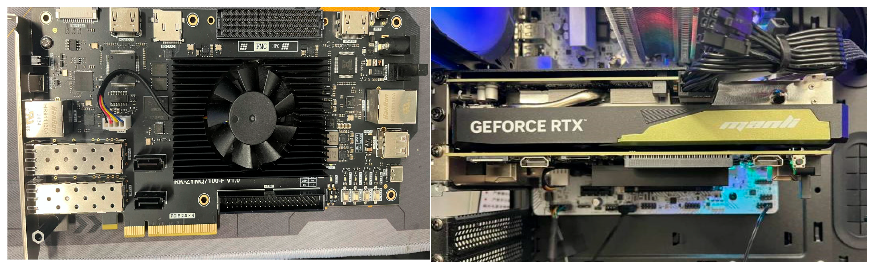
4.1. Experimental Environments

In this work, the proposed solution was implemented on a hardware platform based on the Xilinx Zynq7z100 (San Jose, CA, USA) core, successfully deploying the YOLOv5n network on a hardware accelerator to accomplish the detection task of loose cracks in underground geological structures. To ensure a fair evaluation and comparison of the proposed quantization algorithm across diverse industrial inspection equipment from different domains and datasets, we conducted model accuracy comparisons on the VOC dataset (2007 + 2012) with other FPGA accelerators, with specific details provided in Section 4.3. The training process was performed on the PyTorch 3.12.4 platform, while the accelerator was implemented using Verilog hardware description language (HDL). The design was developed and synthesized in Xilinx Vivado 2023.1, where Register Transfer Level (RTL) code synthesis enabled observation of resource utilization and power consumption. Figure 9 demonstrates the physical FPGA development board connected to the host computer via a PCIe interface for subsurface geotechnical defect detection.

4.2. Dataset

4.2.1. VOC Dataset

The dataset used for accelerator training is the VOC dataset (2007 + 2012) [30]. The PASCAL VOC dataset (2007 + 2012) is a classic benchmark in computer vision, encompassing 20 object categories including humans, animals, vehicles, and indoor objects. This dataset integrates 21,493 annotated images from VOC 2007 and VOC 2012. Its balanced class distribution and standardized evaluation protocols establish it as a gold-standard benchmark for validating model generalizability, particularly in scenarios requiring adaptability to environmental variations such as industrial inspection. The rich annotation details and scene diversity make it an ideal choice for evaluating edge deployment-oriented algorithms like YOLOv5n. Figure 10 shows some sample images from the dataset.

4.2.2. Subsurface Geotechnical Defect-Detection Dataset

This dataset is developed for loose-crack detection tasks in subsurface structural safety assessment, containing two target classes: Crack (rock/concrete cracks) and Loose (loose geotechnical bodies). It contains 1290 annotated geological radar echo images, of which 1022 images are defective, 268 images are defect-free, 716 images have loose defects, and 415 images have crack defects. The dataset effectively validates models’ spatial localization accuracy for cracks and loose regions, providing a critical training and evaluation benchmark for real-time detection of subsurface structural safety hazards in embedded geological radar systems. Figure 11 shows some sample images from the dataset.

4.2.3. Printed Circuit Board (PCB) Defect Dataset

To comprehensively validate the effectiveness and robustness of the proposed method, this study introduces a publicly available synthetic PCB defect dataset released by Peking University. This dataset simulates the complex defect patterns of PCB boards in real electronic manufacturing, covering six common industrial defects: missing_hole, mouse_bite, open_circuit, short, spur, and spurious_copper. The defect area accounts for only 0.5% to 3% of the image area, posing high spatial sensitivity demands on the detector. The dataset consists of 1386 images, divided into training, validation, and test sets in an 8:1:1 ratio to ensure a balanced distribution across categories. Figure 12 shows some sample images from the dataset.

4.3. Training and Inference Results

During the training of the object detection model, a total of 1032 images were used for training, 129 images were employed for real-time evaluation during the training process, and an additional 129 images were reserved as an independent test set to assess the model’s generalization ability. The initial learning rate was optimized and set to 0.001667, with a total of 200 training epochs. Given the limited size of the geological defect dataset (1386 images in total), a multi-dimensional data augmentation strategy was implemented, effectively expanding the training data to more than twice its original volume. Throughout training, key metrics—including the loss function and the mAP@50—were continuously monitored, and the model’s performance on the validation set was automatically evaluated at the end of each epoch. In general, a lower loss and higher mAP indicate better predictive performance of the model. The changes in the loss value and mAP with respect to the number of training epochs are shown in Figure 13.

After 200 epochs of efficient training, the YOLOv5n model demonstrated excellent performance in detecting subsurface geotechnical defects. During the final epoch, the continued decline in key loss functions indicated that the model had fully converged. The model achieved high detection accuracy, with a precision of 96.9%, a recall of 89.7%, and a mAP@50 of 96.2%. Specifically, for the two primary defect types, the model achieved a precision of 97.7%, a recall of 91.2%, and a mAP@50 of 97.6% for “loose bodies”; and a precision of 96.2%, a recall of 88.1%, and a mAP@50 of 94.8% for “cracks”. With a compact model size of only 5.3 MB, it provides an accurate and lightweight solution for monitoring underground structural safety.

The results of geological radar crack and looseness detection are shown in Figure 14. The proposed YOLOv5n heterogeneous parallel accelerator demonstrates excellent detection performance in complex geological environments, validating the effectiveness and practicality of the heterogeneous parallel strategy for geological radar-crack and looseness-detection tasks.

4.4. Analysis and Comparison

Table 2. Layer-wise execution time of YOLOv5 network at different clock frequencies.

100 M		200 M		300 M
Layer	Time/ms	Layer	Time/ms	Layer	Time/ms
Focus	2.801	Focus	2.506	Focus	1.944
Conv1	3.736	Conv1	2.817	Conv1	2.537
Resblock_Body1	10.474	Resblock_Body1	8.024	Resblock_Body1	7.906
Resblock_Body2	10.036	Resblock_Body2	6.784	Resblock_Body2	5.863
Resblock_Body3	11.648	Resblock_Body3	7.186	Resblock_Body3	5.96
Resblock_Body4	8.414	Resblock_Body4	4.813	Resblock_Body4	3.731
SPPF	5.366	SPPF	3.716	SPPF	3.15
Head	33.413	Head	21.026	Head	17.399
Total	85.888	Total	56.872	Total	48.49

presents the execution times of each layer in the YOLOv5 network at clock frequencies of 100 MHz, 200 MHz, and 300 MHz. The experimental results show that with the increase in clock frequency, the execution time of each layer significantly decreases, validating the frequency scalability of the hardware accelerator. The Resblock_Body and Head layers (including multi-scale feature fusion) benefit the most from high-frequency parallel computation, with the greatest performance improvement, thus validating the effectiveness of the heterogeneous parallel architecture. The SPPF layer takes 3.15 ms at 300 MHz, which is a 41.3% reduction compared to 100 MHz. The Head layer takes 17.399 ms, a 47.9% reduction compared to 100 MHz.

As illustrated in

Table 3. The overall resource utilization of the design.

Resource	Utilization	Available	Utilization
LUT	125,956	277,400	45.41%
BRAM	371	755	49.07%
DSP	752	2020	37.23%
FF	177,723	554,800	32.03%

, the implementation consumes 37.23% of DSPs, 32.03% of FFs, 49.07% of block RAMs, and 45.41% of LUTs. The relatively low DSP utilization stems from the 8-bit quantization strategy and bit-serial multiplication optimization, which effectively reduces MAC unit requirements. For the LUT resources, before improving the DSP bit-splitting strategy, the LUT utilization reached 68%. After our optimization, the LUT resource usage was reduced by 33%. In BRAM utilization, a total of 371 instances are used. This reflects the architecture’s high-capacity storage demands for CNN feature map processing, aligning with the requirement for large-scale buffering of intermediate data post-convolution.

The data in

Table 4. Resource utilization and power consumption of computational operators.

	Conv3 × 3	Conv1 × 1	Concat	SPPF	Bottleneck_Add	Focus	Upsample
DSP	576	128	16	None	32	None	None
BRAM	92	63	16	20	12	None	8
FF	78,577	32,651	16,820	7565	17,261	1344	784
LUT	28,598	16,868	14,306	12,216	14,705	776	958
Power/W	0.977	1.105	1.053	0.157	1.314	0.063	0.014

demonstrate that the resource utilization rates of Conv3 × 3 and Conv1 × 1 operators are significantly higher than those of other operators, reflecting their hardware load characteristics as core computational modules in CNNs. In terms of DSP resources, Conv3 × 3 dominates with 576 units, consistent with the theoretical estimation derived from the DSP bit-splitting strategy discussed in Section 3.3:

$${DSP }_{conv33}=input\_num\cdot output\_num\cdot siz{e}^2\cdot {\displaystyle \raisebox{1ex}{$1$}\!\left/ \!\raisebox{-1ex}{$2$}\right.}=16\cdot 8\cdot 9\cdot {\displaystyle \raisebox{1ex}{$1$}\!\left/ \!\raisebox{-1ex}{$2$}\right.}=576$$

(12)

Conv1 × 1 uses 128 units, while BRAM allocation exhibits a similar trend, as shown in Figure 15. This is primarily due to the high-bandwidth access demands of large-scale feature maps and kernel weights in the convolution module. Additionally, the FF and LUT usage of Conv3 × 3 accounts for nearly 50% of the total in the table, combined with its power consumption of 0.977 W, indicating strong dependencies on logic resources due to intensive MAC operations and multi-channel parallel computing. These observations highlight the fact that the hardware implementation of Conv3 × 3 and Conv1 × 1 constitutes a critical bottleneck for system energy-efficiency optimization, necessitating strategies such as operator fusion, data reuse, or quantization compression to reduce resource consumption.

Table 5. Computational performance of 3 × 3 convolutional layers in YOLOv5 network.

Layer	MAC/G	Time/ms	GOPS	Input_Channel	Output_Channel	Stride
Conv3 × 3_layer1	0.356	2.51	141.65	12	16	1
Conv3 × 3_layer2	0.237	1.61	147.03	16	32	2
Conv3 × 3_layer3	0.118	0.55	215.23	16	16	1
Conv3 × 3_layer4	0.236	0.81	291.78	32	64	2
Conv3 × 3_layer5	0.118	0.38	310.97	32	32	1
Conv3 × 3_layer6	0.118	0.38	310.97	32	32	1
Conv3 × 3_layer7	0.236	0.88	268.33	64	128	2
Conv3 × 3_layer8	0.118	0.39	302.74	64	64	1
Conv3 × 3_layer9	0.118	0.39	302.74	64	64	1
Conv3 × 3_layer10	0.118	0.39	302.74	64	64	1
Conv3 × 3_layer11	0.236	1.09	216.54	128	256	2
Conv3 × 3_layer12	0.118	0.37	319.5	128	128	1
Conv3 × 3_layer13	0.11807	0.38	310.7	64	64	1
Conv3 × 3_layer14	0.11817	0.36	328.25	32	32	1
Conv3 × 3_layer15	0.11807	0.45	262.37	64	64	2
Conv3 × 3_layer16	0.11807	0.39	302.74	64	64	1
Conv3 × 3_layer17	0.11801	0.56	210.74	128	128	2
Conv3 × 3_layer18	0.11801	0.36	327.82	128	128	1

shows that, under identical conditions, the GOP/s of convolutional layers with a stride of 2 is significantly lower than those with a stride of 1. For instance, when both input and output channels are 128, conv33_17 exhibits a 35.8% performance degradation compared to conv33_18. This discrepancy primarily stems from the direct impact of stride on the sliding window overlap of convolutional kernels, which governs computational efficiency.

In the row-buffered streaming architecture, when the stride is set to 1, each input row is reused by three consecutive windows with two-row overlaps, achieving a 66.7% buffer reuse rate. This allows a single input pixel to be reused up to nine times, maximizing on-chip BRAM utilization and minimizing redundant data reloading. However, when the stride is set to 2, the increased sliding interval reduces pixel reuse to approximately 2.25 times, significantly decreasing data reuse efficiency. The lower reuse rate leads to more frequent switching of input data blocks, diminishing the benefits of on-chip caching.

Table 6. Comparative analysis of accelerator performance against existing works.

	[31]	[17]	[32]	[14]	[33]	[34]	This Work
Platform	Zynq XCZU7EV	Xilinx ZC706	Zynq XCZU7EV	Xilinx ZC709	ZYNQ- 7020	KCU116	Zynq XC7Z100
Network	AlexNet	Tiny YOLO-V2	Tiny YOLO-V3	Tiny YOLO-V3	Tiny YOLO-V4	YOLO- V5s	YOLO-V5n
Operation Frequency	300 MHz	100 MHz	166 MHz	200 MHz	None	None	300 M
Arithmetic Precision	8	16–32	16	16	16	TT	8
BRAM	198.5	301	254	624	96	220	370
DSP	696	784	46	514	216	1321	752
LUT	101,953	182,086	117,696	176,130	41,953	182,000	216,725
FF	127,577	132,869	117,157	140,012	47,652	123,098	224,544
Throughput (GOPs)	14.11	41.99	42.5	120	9.24	42.6	157.04
Power (W)	17.67	7.5	4.96	7.36	2.86	15.3	9.4
Energy Efficiency (GOPs/W)	0.8	5.6	8.57	16	3.23	2.8	16.7

demonstrates the resource consumption and performance comparison between our proposed accelerator and those from other studies. Since we aim to perform a board-level demonstration, this solution inevitably uses some system modules that do not participate in the main CNN computation. For example, the FPGA communicates with the CPU via the PCIe interface, which adds overhead beyond the computation, occupies part of the on-chip memory, and affects the overall operating frequency. Despite this, the throughput of our design can still reach 157.04 GOPs, with an energy efficiency of 16.7 GOPs/W, which still offers multiple advantages compared to other solutions. The detailed comparison is provided below.

Although the method proposed in [31] reduces on-chip resource consumption by recovering the original sparse matrix at an operating frequency of 300 MHz, its high power dissipation and dependence on specific computational patterns severely limit its practicality for real-time vision tasks. In contrast, our design achieves a fundamental balance between efficiency and computational capacity, by completely eliminating reliance on sparse matrix recovery. Through the adoption of a dense computation paradigm combined with optimized data reuse and parallelization strategies, our framework attains a 20.9× improvement in energy efficiency (16.7 GOPS/W vs. 0.8 GOPS/W) under the same clock frequency. The accelerator in [17], targeting the YOLO v2-tiny network, employs a data block transmission strategy and dual 14 × 14 PE matrices, along with an enhanced roofline model to optimize the balance between computation and memory bandwidth. On the Xilinx ZC706 platform at 100 MHz, it achieves a throughput of 41.99 GOPS and an energy efficiency of 5.6 GOPS/W. However, its mixed 16/32-bit precision design fails to fully exploit the potential of low-bit quantization. In [32], a zero-padding strategy is applied in hardware to mitigate on-chip memory constraints and reduce data transmission overhead. Similarly, our design implements zero-padding for the remaining four channels in the Focus layer. The work in [14] proposed a CPU-FPGA hybrid architecture for CNN acceleration, utilizing a 32 × 16 DSP streaming array for parallel convolution. However, the efficiency of this general-purpose DSP streaming array is constrained by variations in kernel sizes. In contrast, our solution adopts a heterogeneous parallel acceleration strategy tailored to different kernel sizes, achieving an energy efficiency of 16.7 GOPS/W—4.4% higher than the 16 GOPS/W reported in [15]—while providing hardware-agnostic support for dynamic multi-model deployment, thereby overcoming bottlenecks in cooperative scheduling within hybrid architectures.

Researchers in [33] adopted three optimization methods: input–output channel parallelism, pipelining, and ping-pong operation, and used a 16-bit quantization strategy. Since the bit-width of the quantization is higher than the 8-bit quantization used in this approach, and Vivado HLS design is employed, the throughput performance is relatively poorer due to this high-level synthesis method. Researchers in [34] proposed an innovative specialized hardware architecture based on the unique characteristics of tensor train decomposition, achieving higher computation efficiency. In comparison, although our approach utilizes more BRAM and LUT resources, it achieves 6× higher energy efficiency than their solution.

Table 7. Performance comparison analysis table of FPGA-based CNN accelerators and GPUs.

	GPU	FPGA
Device model	NVIDIA RTX 3090	Xilinx Zynq7z100
Throughput (GOPs)	1075	157
Power (W)	170	9.4
Energy Efficiency (GOPs/W)	6.32	16.7

compares the advantages of FPGA in edge computing applications. The NVIDIA RTX 3090 GPU (Santa Clara, CA, USA) offers high computational power, achieving a throughput of 1075 GOPs, but its power consumption of 170W results in an energy efficiency ratio of just 6.32 GOPs/W. In contrast, the Xilinx Zynq7z100 FPGA delivers 157 GOPs of inference performance with a remarkably low power consumption of just 9.4W, yielding an energy efficiency ratio of 16.7 GOPs/W—2.64 times higher than that of the GPU. This demonstrates the engineering value of heterogeneous parallel strategies in edge computing.

5. Conclusions

This paper introduces an enhanced YOLOv5n FPGA accelerator architecture, deployed on the Xilinx Zynq7z100 platform, for detecting subsurface geotechnical defects. The proposed approach optimizes buffer design to minimize redundant data reloading. A heterogeneous parallel strategy is implemented for different convolution operations: a 16 × 8 hybrid architecture is used for 3 × 3 convolutions, while 1 × 1 convolutions and other operations utilize a 16 × 16 configuration. Additionally, by reconfiguring the input port mapping of Xilinx DSP48E2 units, dual-channel 8-bit fixed-point multiply–accumulate operations are supported within a single DSP, which reduces LUT resource consumption. In the actual deployment, 752 DSPs are employed. The system operates at a clock frequency of 300 MHz, achieving a peak throughput of 328.25 GOPs in convolution layers, an overall throughput of 157.04 GOPs, an end-to-end inference latency of 48.49 ms per frame, power consumption of 9.4 watts, energy efficiency of 16.7 GOPs/W, and a 33% reduction in LUT resource usage. This paper provides a flexible, low-power hardware acceleration paradigm for object detection in edge computing, with a particular focus on its application in subsurface geotechnical defect-detection scenarios that require strict real-time and energy-efficiency standards.

References

1. Li, B.; Chu, X.; Lin, F.; Wu, F.; Jin, S.; Zhang, K. A highly efficient tunnel lining crack detection model based on Mini-Unet. Sci. Rep. 2024, 14, 28234. [Google Scholar] [CrossRef] [PubMed]
2. Zhou, Z.; Zhang, J.; Gong, C. Hybrid semantic segmentation for tunnel lining cracks based on Swin Transformer and convolutional neural network. Comput.-Aided Civ. Infrastruct. Eng. 2023, 38, 2491–2510. [Google Scholar] [CrossRef]
3. Fu, Y.; Liu, Y.; Chen, G. Stability analysis of rock slopes based on CSMR and convolutional neural networks. J. Nat. Disasters 2023, 32, 114–121. [Google Scholar]
4. Lin, M.; Chen, X.; Chen, G.; Zhao, Z.; Bassir, D. Stability prediction of multi-material complex slopes based on self-attention convolutional neural networks. Stoch. Environ. Res. Risk Assess. 2024, 1–17. [Google Scholar] [CrossRef]
5. Guo, W.; Zhang, X.; Zhang, D.; Chen, Z.; Zhou, B.; Huang, D.; Li, Q. Detection and classification of pipe defects based on pipe-extended feature pyramid network. Autom. Constr. 2022, 141, 104399. [Google Scholar] [CrossRef]
6. Ghodhbani, R.; Saidani, T.; Zayeni, H. Deploying deep learning networks based advanced techniques for image processing on FPGA platform. Neural Comput. Appl. 2023, 35, 18949–18969. [Google Scholar] [CrossRef]
7. Kumari, N.; Ruf, V.; Mukhametov, S.; Schmidt, A.; Kuhn, J.; Küchemann, S. Mobile eye-tracking data analysis using object detection via YOLO v4. Sensors 2021, 21, 7668. [Google Scholar] [CrossRef]
8. Ma, J.; Zhou, Y.; Zhou, Z.; Zhang, Y.; He, L. Toward smart ocean monitoring: Real-time detection of marine litter using YOLOv12 in support of pollution mitigation. Mar. Pollut. Bull. 2025, 217, 118136. [Google Scholar] [CrossRef]
9. Tu, C.; Yi, A.; Yao, T.; He, W. High-precision garbage detection algorithm of lightweight yolov5n. Comput. Eng. Appl. 2023, 59, 187–195. [Google Scholar]
10. Feng, Y.; Zhao, X.; Tian, R.; Liang, C.; Liu, J.; Fan, X. Research on an Intelligent Seed-Sorting Method and Sorter Based on Machine Vision and Lightweight YOLOv5n. Agronomy 2024, 14, 1953. [Google Scholar] [CrossRef]
11. Chen, Z.; Lin, Y.; Xu, J.; Lu, K.; Huang, Z. A fused score computation approach to reflect the overlap between the predicted box and the ground truth in pedestrian detection. IET Image Process. 2024, 18, 4287–4296. [Google Scholar] [CrossRef]
12. Zhang, Y.; Guo, Z.; Wu, J.; Tian, Y.; Tang, H.; Guo, X. Real-time vehicle detection based on improved yolo v5. Sustainability 2022, 14, 12274. [Google Scholar] [CrossRef]
13. He, K.; Zhang, X.; Ren, S.; Sun, J. Deep residual learning for image recognition. In Proceedings of the IEEE Conference on Computer Vision and Pattern Recognition, Las Vegas, NV, USA, 27–30 June 2016; pp. 770–778. [Google Scholar]
14. Guo, Z.; Gao, Y.; Hu, H.; Gong, D.; Liu, K.; Wu, X. Research on Acceleration of Convolutional Neural Network Algorithm Based on Hybrid Architecture. J. Comput. Eng. Appl. 2022, 58, 88–94. [Google Scholar]
15. Zhang, D.; Wang, A.; Mo, R.; Wang, D. End-to-end acceleration of the YOLO object detection framework on FPGA-only devices. Neural. Comput. Appl. 2024, 36, 1067–1089. [Google Scholar] [CrossRef]
16. Valadanzoj, Z.; Daryanavard, H.; Harifi, A. High-speed YOLOv4-tiny hardware accelerator for self-driving automotive. J. Supercomput. 2024, 80, 6699–6724. [Google Scholar] [CrossRef]
17. Huang, H.; Liu, Z.; Chen, T.; Hu, X.; Zhang, Q.; Xiong, X. Design space exploration for yolo neural network accelerator. Electronics 2020, 9, 1921. [Google Scholar] [CrossRef]
18. Shafiei, M.; Daryanavard, H.; Hatam, A. Scalable and custom-precision floating-point hardware convolution core for using in AI edge processors. J. Real-Time Image Process. 2023, 20, 94. [Google Scholar] [CrossRef]
19. Yan, Z.; Zhang, B.; Wang, D. An FPGA-Based YOLOv5 Accelerator for Real-Time Industrial Vision Applications. Micromachines 2024, 15, 1164. [Google Scholar] [CrossRef]
20. Kim, M.; Oh, K.; Cho, Y.; Seo, H.; Nguyen, X.T.; Lee, H.-J. A low-latency FPGA accelerator for YOLOv3-tiny with flexible layerwise map and dataflow. IEEE Trans. Circuits Syst. I Regul. Pap. 2023, 71, 1158–1171. [Google Scholar] [CrossRef]
21. Guo, R.; Liu, H.; Xie, G.; Zhang, Y. Weld defect detection from imbalanced radiographic images based on contrast enhancement conditional generative adversarial network and transfer learning. IEEE Sens. J. 2021, 21, 10844–10853. [Google Scholar] [CrossRef]
22. Dai, W.; Wang, Y.; Li, X.; Wang, Y. YOLO aluminum profile surface defect detection system for FPGA deployment. J. Electron. Meas. Instrum. 2023, 37, 160–167. [Google Scholar]
23. Johnson, V.C.; Bali, J.; Chanchal, A.K.; Kumar, S.; Shukla, M.K. Performance Comparison of Machine Learning Classifiers for FPGA-Accelerated Surface Defect Detection. In Proceedings of the 2024 IEEE Conference on Engineering Informatics (ICEI), Melbourne, Australia, 20–28 November 2024. [Google Scholar]
24. Ding, Z.; Liu, C.; Li, D.; Yi, G. Deep-sea biological detection method based on lightweight YOLOv5n. Sensors 2023, 23, 8600. [Google Scholar] [CrossRef] [PubMed]
25. Liu, Z.; Hu, X.; Xu, L.; Wang, W.; Ghannouchi, F.M. Low computational complexity digital predistortion based on convolutional neural network for wideband power amplifiers. IEEE Trans. Circuits Syst. II Express Briefs 2021, 69, 1702–1706. [Google Scholar] [CrossRef]
26. Wei, S.X.; Yu, H.; Zhang, P. A farmed fish detection method based on a non-channel-downscaling attention mechanism and improved YOLOv5. Fish. Mod. 2023, 50, 72–78. [Google Scholar]
27. Zhang, H.; Shao, F.; He, X.; Zhang, Z.; Cai, Y.; Bi, S. Research on object detection and recognition method for UAV aerial images based on improved YOLOv5. Drones 2023, 7, 402. [Google Scholar] [CrossRef]
28. Chen, L.; Lou, P. Clipping-Based Post Training 8-Bit Quantization of Convolution Neural Networks for Object Detection. Appl. Sci. 2022, 12, 12405. [Google Scholar] [CrossRef]
29. Wang, J.; Fang, S.; Wang, X.; Ma, J.; Wang, T.; Shan, Y. High-performance mixed-low-precision cnn inference accelerator on fpga. IEEE Micro 2021, 41, 31–38. [Google Scholar] [CrossRef]
30. Everingham, M.; Eslami, S.A.; Van Gool, L.; Williams, C.K.; Winn, J.; Zisserman, A. The pascal visual object classes challenge: A retrospective. Int. J. Comput. Vis. 2015, 111, 98–136. [Google Scholar] [CrossRef]
31. Zhang, M.; Li, L.; Wang, H.; Liu, Y.; Qin, H.; Zhao, W. Optimized compression for implementing convolutional neural networks on FPGA. Electronics 2019, 8, 295. [Google Scholar] [CrossRef]
32. Tsai, T.H.; Tung, N.C.; Chen, C.Y. An FPGA-Based Reconfigurable Convolutional Neural Network Accelerator for Tiny YOLO-V3. Circuits Syst. Signal Process. 2025, 44, 3388–3409. [Google Scholar] [CrossRef]
33. Xu, S.; Zhou, Y.; Huang, Y.; Han, T. YOLOv4-tiny-based coal gangue image recognition and FPGA implementation. Micromachines 2022, 13, 1983. [Google Scholar] [CrossRef] [PubMed]
34. Liu, M.; Luo, S.; Han, K.; Yuan, B.; DeMara, R.F.; Bai, Y. An efficient real-time object detection framework on resource-constricted hardware devices via software and hardware co-design. In Proceedings of the 2021 IEEE 32nd International Conference on Application-Specific Systems, Architectures and Processors (ASAP), Online, 7–9 July 2021; pp. 77–84. [Google Scholar]
Figure 1. Structure of YOLOv5n.
Electronics 14 02585 g001
Figure 2. Structure of CSP.
Electronics 14 02585 g002
Figure 3. Overall structure of the proposed accelerator.
Electronics 14 02585 g003
Figure 4. Row buffering mechanism.
Electronics 14 02585 g004
Figure 5. Flowchart of DSP bit-width partitioning scheme before improvement.
Electronics 14 02585 g005
Figure 6. Specific bit allocation of the improved DSPE1 high-bit-width partitioning scheme.
Electronics 14 02585 g006
Figure 7. 3 × 3 convolution acceleration strategy.
Electronics 14 02585 g007
Figure 8. PE design for 3 × 3 convolution.
Electronics 14 02585 g008
Figure 9. Experimental hardware setup.
Electronics 14 02585 g009
Figure 10. Sample images from the VOC dataset.
Electronics 14 02585 g010
Figure 11. Sample images from the subsurface geotechnical defect-detection dataset.
Electronics 14 02585 g011
Figure 12. Sample images from the PCB defect dataset.
Electronics 14 02585 g012
Figure 13. TrainingEpoch–Lossdiagrams and TrainingEpoch–mAPdiagrams.
Electronics 14 02585 g013
Figure 14. Detection results of geophysical radar detect.
Electronics 14 02585 g014
Figure 15. 3D line chart of the resource and power distribution percentage of various operators in the FPGA accelerator.
Electronics 14 02585 g015