1. Introduction
Permanent magnet synchronous motors (PMSMs) are widely used in various fields due to their advantages such as high efficiency, high control accuracy, and good dynamic performance [
1]. Due to the benefits of the high power density and wide speed regulation range of high-speed permanent magnet synchronous motors, they display great application potential in the motor vehicle, fan, and aerospace industries [
2,
3]. To achieve high-performance control of PMSMs, the control system relies on accurate position information. Position sensors not only increase the cost of the system but are also susceptible to external environmental influences. Moreover, the higher mechanical strength requirements for sensors imposed by high rotational speeds often render rotor position sensors on high-speed shafts either impractical or infeasible to install [
3]. In contrast, sensorless control systems can reduce the cost and improve the reliability of the system. Therefore, sensorless control systems have become a research hotspot in the past few decades [
4,
5].
In the medium to high-speed range studied in this paper, sensorless control systems typically use model-based observer methods to obtain position information [
4,
6,
7,
8,
9]. Most observers are designed using continuous-domain motor mathematical models [
6,
10,
11] and run on microcontroller units (MCUs). In applications where the ratio of sampling frequency to fundamental frequency, i.e., the carrier–frequency ratio (CFR), is high, these observers perform well in terms of accuracy. However, as the speed increases, these observers exhibit accuracy issues [
5,
12,
13]. For example, ultra-high-speed motors used in wind turbines and high-pole-count motors used in electric vehicles may display maximum operating fundamental frequencies close to or even exceeding 1 kHz [
14]. However, due to the limitations of power switch device switching losses and MCU performance [
12,
15,
16], the sampling frequency cannot be increased indefinitely as the motor’s fundamental frequency increases, forcing the CFR to decrease. An excessively low CFR can lead to a decrease in the accuracy of the discrete mathematical model, which in turn degrades the performance and even the stability of the discrete observer [
5]. Therefore, it is crucial to design a discrete observer with good stability and accuracy under low CFR.
To improve observer performance, references [
5,
13] suggest designing the observer in the discrete-time domain under low CFR. In reference [
10], the Tustin approximate method was used to design a Luenberger observer, and the performance of observers designed using the Euler method and the Tustin method was compared. The stability and accuracy of the observer designed using the Tustin method was improved, and the steady-state and dynamic performance of the control system were also enhanced. Reference [
17] points out that when the CFR drops to a certain level, this approximate method also introduces estimation errors, and the observer should be designed directly using a discrete model of PMSM. Reference [
18] mentions that using a more accurate discrete-time model to design a flux observer at low CFR can achieve accurate stator flux estimation and good dynamic performance, yielding results comparable to those of high CFR observers. Reference [
19] shows that a current observer designed using a discrete model can remain stable and maintain a certain level of accuracy even at a CFR of 12. To obtain a discrete observer with high accuracy at a low CFR, the discrete motor model is usually derived from the solution of the continuous system state equation. Assuming that the input voltage and back EMF are constant over a sampling period, the resulting discrete model is the motor zero-order hold (ZOH) discrete model. Reference [
20] designed a discrete sliding mode observer using this method, which remained stable at a CFR of 10. Reference [
21] considered voltage compensation and designed a discrete full-order observer using the motor ZOH discrete model, improving position observation performance by 2.5 times under no-load conditions. To further improve the accuracy of the motor discrete mathematical model, reference [
17] replaced the change in back EMF over a sampling period with the average back EMF over the sampling period to enhance accuracy. However, this method still has modeling errors. Further, reference [
22] assumed that the amplitude of the back EMF does not change over a sampling period and derived an accurate discrete mathematical model based on this assumption. This model has very small position errors at a CFR of 10. Reference [
23] designed a deadbeat back EMF observer using the accurate discrete mathematical model, achieving excellent results at a CFR of 10. However, the accurate discrete mathematical models in references [
22,
23] were derived in complex form and did not utilize the phase information from the back EMF non-homogeneous solution.
This paper derives the accurate discrete mathematical model of a surface-mounted PMSM (SPMSM) in the real number domain and provides the mathematical expression for phase compensation related to the non-homogeneous solution of back EMF. Based on this model, an accurate discrete Luenberger observer (ALO) is designed. Experiments compare the position estimation accuracy of the ALO with that of the traditional Luenberger observer (TLO) using Euler discretization at high and low CFRs. Comparative experiments indicate that the ALO reduces the position error by 80%, 87.6%, and 89.3% at CFRs of 30, 18, and 12.27, respectively. ALO significantly enhances the accuracy of the estimated position, demonstrating that accurate discrete motor model improves the performance of the observer.
2. Accurate Discrete Mathematical Model
The continuous mathematical model of SPMSM is given as [
6]
where
are the currents in the α and β axes of the two-phase stationary coordinate system (A);
are the input voltages in the α and β axes (V);
are the back EMF in the α and β axes (V);
R is the phase resistance of the motor (Ω);
L is the phase inductance of the motor (H);
is the permanent magnet flux linkage of the rotor (Wb);
ω is the electrical angular velocity of the motor (rad/s);
θ is the rotor position of the motor, i.e., the angle formed between the rotor and the α-axis (rad). It is expressed in the standard state-space equation form as follows:
where
x is the state variable;
w is the input vector;
u is the voltage vector;
E is the back EMF vector;
Ac is the system matrix;
Bc is the input matrix;
I is the unit matrix;
A is −R/L.
When the sampling period
T is very short, the Euler method, i.e., the forward difference method, can be used to obtain an approximate discrete mathematical model.
In the following, the sampling time,
kT is abbreviated as
k, where
k is the sampling sequence. By substituting Equation (3) into Equation (2), the discrete mathematical model based on the Euler approximation can be obtained as
When the motor speed increases to a certain level, the CFR of the motor is relatively small. Then, the discrete model obtained using the Euler approximation method is no longer accurate.
According to modern control theory, the discrete state equation for a system of the form given in Equation (2) can be expressed as [
20]
Equation (5) is decomposed as follows:
where
represents the non-homogeneous solution of the voltage and back EMF from time
k to
k + 1.
For solving the function, since the motor rotor has a certain moment of inertia, the speed does not change significantly within one sampling period. For the control system of the high-speed permanent magnet synchronous motor mentioned in reference [
11], the sampling period is 100 us, and the rotor moment of inertia is 0.02 kg·m. If within one sampling period, the rotational speed of the motor fluctuates only within 1% of the rated speed, that is, 215 RPM, the torque of the motor needs to change by 4502 N·m. For a motor with a moment of inertia of only 0.00094 kg·m
2 [
7], for the same change in rotational speed, the torque needs to change by 211 N·m. Therefore, the rotational speed of the motor is difficult to change significantly within one sampling period. Thus, it is assumed that the motor speed remains constant within one sampling period, meaning that the amplitude of the back EMF remains unchanged. Thus, the back EMF can be regarded as a standard sinusoidal wave within one sampling period, i.e.,
Substituting Equation (7) into Equation (8) yields
where
represents the non-homogeneous solution of the back EMF in the α and β axes from time
k to
k + 1;
is the phase offset indicating the phase relationship between
and the
;
is the amplitude scaling expressing the amplitude relationship between
and the
. To visually represent the differences between the two, simulation software was used to simulate
and
, and the results are shown in
Figure 1. In the simulation, an eight-pole SPMSM is adopted. Its parameter
A is −500, and the permanent magnet flux linkage
is 0.0128 Wb. The sampling period
T is set to 1.11 ms, and the electrical angular velocity
of the SPMSM is controlled to be maintained at 420. It can be seen from
Figure 1 that there are obvious differences between
and
. At this time, the
is −0.2521 rad, and the
is 8.4 × 10
−4.
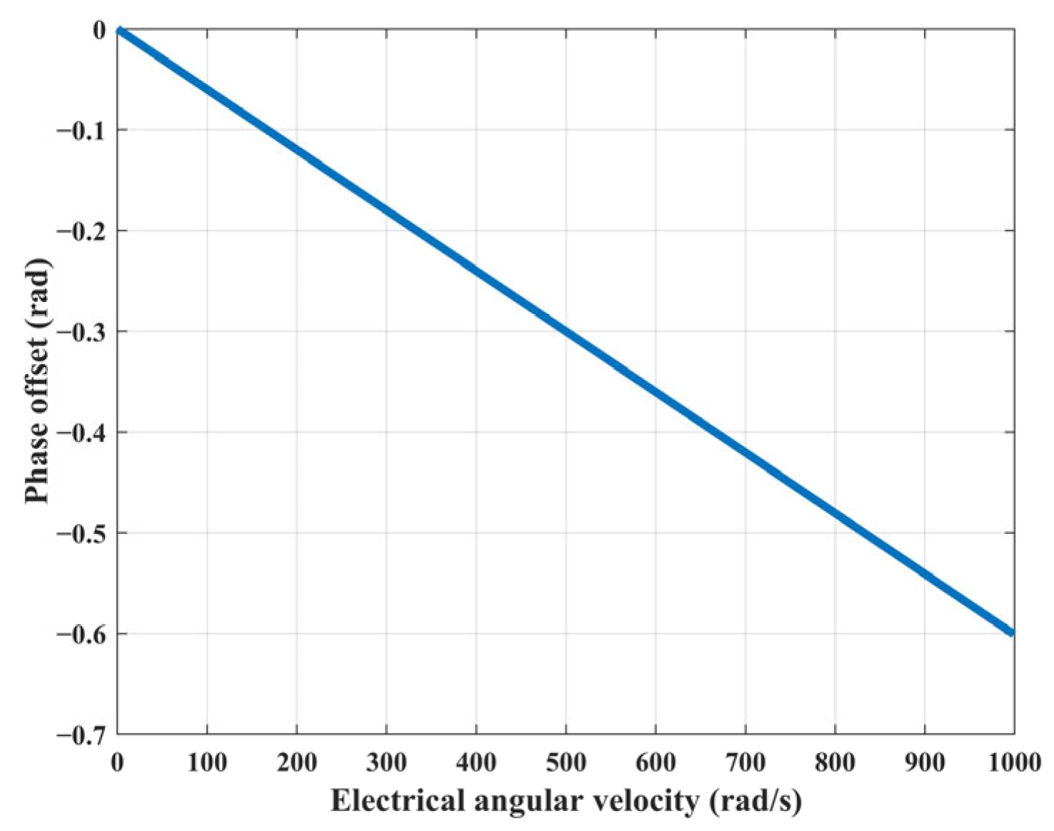
According to Equation (10), it can be seen that when the rotational speed of the motor is higher, that is, when the carrier–frequency ratio decreases, the phase difference between
E(
k) and
is greater.
Figure 2 shows the relationship between electrical angular velocity and phase offset when
A is −500 and
T is 1.11 ms.
According to Equation (9), it can be observed that once
is obtained, the rotor position at time
k can be obtained. However, due to the phase difference between
and
, after obtaining
using the current information and
, the arctangent values of
and
cannot be directly taken as the actual rotor position, as in the traditional method. In order to obtain the actual rotor position, it is necessary to perform phase
compensation correction on the arctangent of
and
, that is, Equation (11). Since
plays a compensating role when calculating the rotor position, it will also be referred to as the phase compensation value in the subsequent text.
For solving the function
, since the motor driver is controlled by PWM, when the sampling period is the same as the PWM period, the input voltage
u can be considered constant within one sampling period. Therefore, the solution for
can be simplified as follows:
where
represents the non-homogeneous solution of the voltage in the α and β axes from time
k to
k + 1. Considering that the updated PWM command within the sampling period takes effect in the next sampling period [
13,
14], the accurate discrete mathematical model is given as follows:
By comparing this calculation with Equation (4), it can be observed that it represents the Taylor series expansion form of Equation (13). It can also show that the rotational speed and sampling period affect the accuracy of discrete mathematical models. The specific calculation of Equation (13) is
3. Accurate Discrete Luenberger Observer
The Luenberger observer is used to estimate the motor states and calculate the rotor position. The mathematical expression of the Luenberger observer is provided in reference [
24] as follows:
where
represents the observer’s state variables;
represents the observer’s output variables;
y is the actual system output;
C is the output matrix;
is the extended system matrix;
is the observer input matrix;
K is the observer’s feedback gain matrix;
are the estimated currents in the α and β axes;
are the estimated back EMFs in the α and β axes. To observe the rotor position of the motor,
should be included as two states of the observer’s state variables. From Equation (1),
and
can be determined as follows:
In order to prevent the poles of the observer from changing significantly with the variation of the motor speed and to improve the observer’s adaptive ability to speed, according to reference [
25], the feedback gain matrix
K of the observer is designed as
It can be observed from Equation (15) that the state matrix of the observer
is
To ensure the stability of the observer and to provide the observer with an accelerated convergence rate, its poles are designed as
, that is
since
the feedback gain matrix
K can be determined by solving Equation (23).
Thus, the feedback gain matrix
K can be obtained as
For the discretization of
, since
using Equation (6) and assuming that the rotational speed is constant over a sampling period, Equation (26) will be obtained.
The second-order Taylor series expansion is used to linearize Equation (26). After linearization, the discrete equation for
becomes
Combining the accurate discrete mathematical model, Equation (14), the mathematical expression of the ALO can be derived as
where
represents the ALO’s state variables, and
represents the estimated electrical angular velocity at time
k; the feedback gain matrix
is
To highlight the superiority of the ALO in terms of observation accuracy under low CFR, the discrete expression of the TLO obtained through Equation (3) and Euler approximation is provided by reference [
10]. Considering the PWM command update delay, its expression is as follows
4. Experimental Verification
The ALO primarily addresses the issue of observer accuracy under low CFR. For convenience, a common SPMSM was used instead of a high-speed PMSM for the experiment. The parameters of the motor used in the experiment are shown in
Table 1. Since most common SPMSMs are designed with speeds ranging from 3000 to 5000 RPM and are typically four-pole motors, the sampling frequency is usually 10 kHz, resulting in a CFR of about 60. For high-speed PMSMs, their rotational speeds typically exceed 20,000 RPM, while the CFR is generally below 30 [
3,
11,
21]. Therefore, such a high CFR of the common SPMSM does not conform to the actual working conditions of a high-speed PMSM. To simulate the low CFR control system, the control period, PWM carrier frequency, and ADC sampling frequency were set to 900 Hz. The experiments were conducted at speeds of 450 RPM, 750 RPM, and 1100 RPM, corresponding to CFRs of 30, 18, and 12.27, respectively, to compare the accuracy of the TLO and the ALO.
To visually compare the accuracy differences between the TLO and the ALO, the experiment utilizes the arctangent function to calculate the estimated rotor position. The estimated position for the ALO is calculated using Equation (31), while the traditional method uses Equation (32). The estimated electrical angular velocity is solved by the difference quotient of the estimated position, Equation (33), and then obtained by a digital first-order low-pass filter with a bandwidth of 40π, Equation (34).
where
represents the estimated position of the ALO at time
k + 1;
represents the estimated position of the TLO at time
k + 1.
where
represents the estimated position of the ALO or TLO at time
k + 1;
is the original estimated electrical angular velocity of the ALO or TLO at time
k + 1.
where
represents the estimated electrical angular velocity for the ALO or TLO;
is the bandwidth of the digital first-order low-pass filter.
The experimental platform setup is shown in
Figure 3. The DSP28335 control box is used to implement the digital control of the motor, and the ALO and TLO are constructed in the DSP, according to Equations (28) and (30). The current of the SPMSM is measured using an ACS711ELCTR Hall sensor, which has a maximum detectable current of 25 A. The actual rotor position is provided by an incremental encoder with a resolution of 2500 PPR, serving as a benchmark for measuring the accuracy of the estimated position. In the control strategy, a PI controller is employed to directly regulate the rotational speed of the SPMSM. The proportional gain is configured to four, while the integral gain is set to eight. The output of the PI controller serves as the reference value for the q-axis voltage
, and the reference value for the d-axis voltage is established at 0 V. The inverter adopts the space vector pulse width modulation algorithm to enable the SPMSM to obtain the actual q-axis
and d-axis voltages. At the same time, it is highly challenging for the rotational speed of an actual high-speed PMSMs to undergo significant variation within a single sampling period. Nevertheless, the sampling frequency employed in this experiment was 900 Hz, which makes it more probable for the motor’s rotational speed to change considerably within one sampling period. Consequently, even in the no-load experimental setup, a brushed DC motor was connected in the system as a loading device. This was done in order to increase the moment of inertia of the tested SPMSM, thereby mitigating the fluctuation of rotational speed during a single sampling period. Finally, the data generated in the experiment, such as the actual position, estimated position, estimated position error, rotor position compensation, actual speed, estimated speed, a-phase current, and load torque, are sent to a personal computer (PC) by the DSP28335 at a frequency of 1 KHz through the serial communication interface (SCI) for analysis and storage.
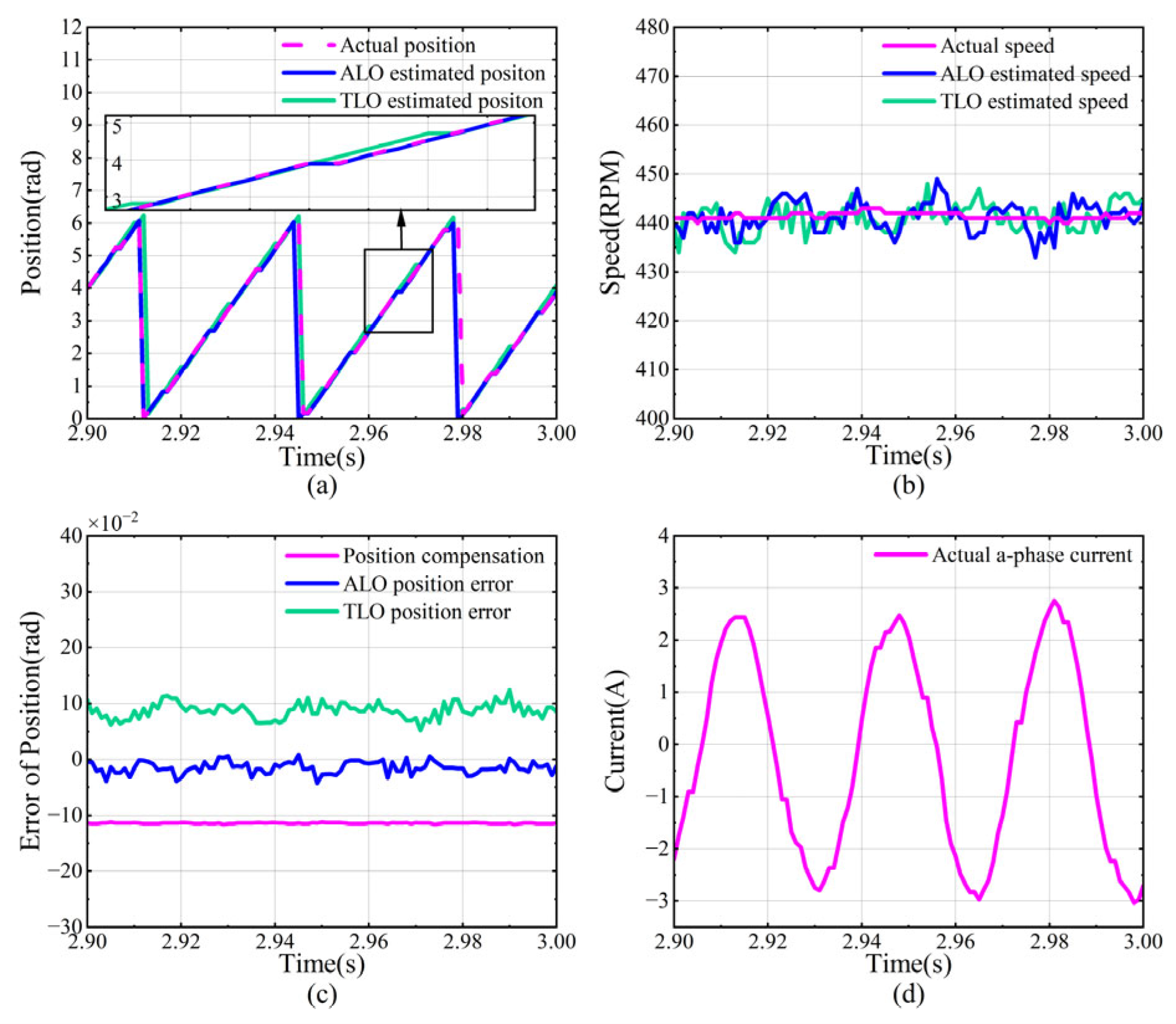
The following are four groups of no-load experiments. First, the performance of both observers is compared under a high CFR. The target speed is set to 450 RPM (CFR of 30). Under this condition, the motor speed stabilizes in approximately 3 s. Data from 2.9 to 3 s is selected to evaluate the performance of the ALO and TLO under steady-state conditions, including the estimated position, estimation position error, and estimated speed. The a-phase current of the motor during this period is recorded and shown in
Figure 4.
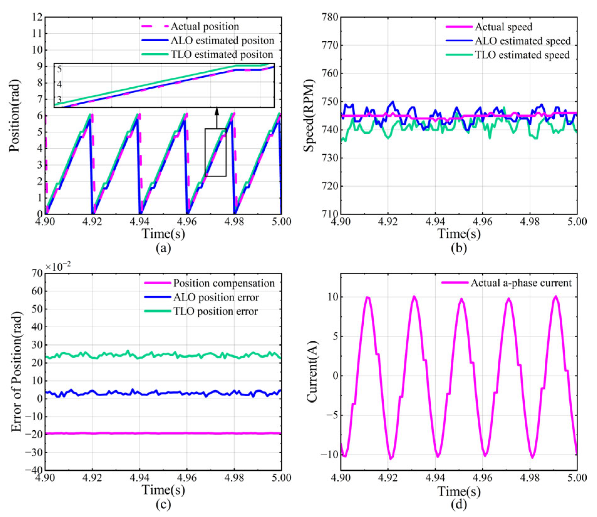
The target speed is increased to 750 RPM (CFR of 18), and the motor speed stabilizes in approximately 5 s. Data from 4.9 to 5 s is selected to evaluate the performance of the ALO and TLO under steady-state conditions, as shown in
Figure 5.
The target speed is increased to 1100 RPM (CFR of 12.27), pushing the current to the measurable limit of the control system. The motor speed stabilizes in approximately 6.5 s. Data from 6.4 to 6.5 s is selected to evaluate the performance of the ALO and TLO under steady-state conditions, as shown in
Figure 6. In
Figure 6d, it can be observed that at a CFR of 12.27, the current exceeds 25 A. The positive current measured by the DSP through the ADC is limited to 25 A, while the negative peak reaches around −27 A, causing distortion in the current signals obtained by the ALO and TLO.
Through statistical analysis, the errors under steady-state conditions for the three sets of experiments are summarized in
Table 2, with the angular units converted from radians (rad) to degrees (°). From
Table 2, by comparing the mean position errors of the TLO and ALO across the three experiments, it can be concluded that the position compensation of the ALO plays a significant role in improving accuracy. This also demonstrates that designing an observer using accurate modeling is crucial for enhancing precision. As the CFR decreases, the absolute value of the position compensation gradually increases, enabling the ALO to maintain small estimation position errors at both high or low CFR. In the experiments, the estimation position error of the ALO remained below 2°, while the maximum error of the TLO reached 17°. Furthermore, as the CFR decreases, the gap in accuracy between the TLO and the ALO widens. Specifically, at a CFR of 30, the root mean square (RMS) position error of the ALO is 20% lower than that of the TLO; at a CFR of 18, it is 12.4%, and at a CFR of 12.27, it is 10.7%. This indicates that the advantages of the ALO become more pronounced as the CFR decreases.
To demonstrate the performance of the ALO and TLO under dynamic speed variations, the actual speed, ALO estimated speed, TLO estimated speed, a-phase current, ALO position compensation, and position errors of ALO and TLO at a CFR of 12.27 are shown in
Figure 7. As the motor speed increases, the position error of the TLO gradually increases, while the ALO is less affected by speed variations. Additionally, the position compensation of the ALO decreases as the speed increases. However, since the accurate discrete model does not account for the influence of angular acceleration, there is a relatively large position error during significant speed changes, particularly within the 0–1 s interval shown in
Figure 7. Furthermore, as illustrated in
Figure 7, current distortion occurs around 4 s. When the current signal of the observer becomes distorted, the position accuracy of the TLO significantly deteriorates, while the ALO is less affected.
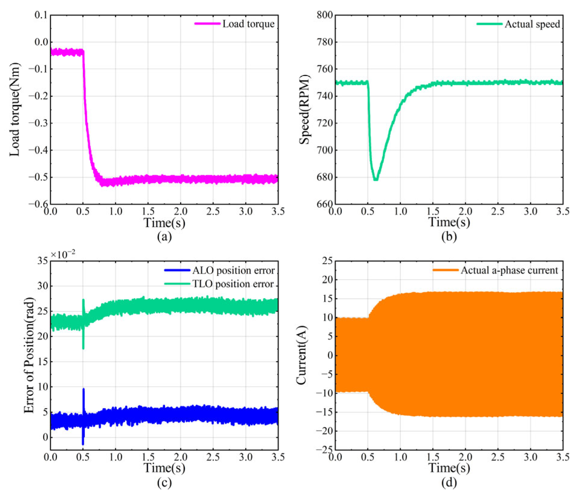
To evaluate the performance of ALO under sudden load variations, loading experiments were conducted at a rotational speed of 750 RPM, corresponding to a CFR of 18. As illustrated in
Figure 8, at 0.5 s, a load torque of 0.5 N·m was applied to the tested SPMSM using a brushed DC motor. The changes in load torque, actual speed, ALO position error, TLO position error, and a-phase current were subsequently recorded. When the load torque undergoes a sudden change, the speed decreases sharply by approximately 70 RPM within 0.2 s. During this interval, due to the abrupt variation in rotational speed, both the ALO position error and the TLO position error exhibit significant fluctuations. However, the ALO position error remains smaller than the TLO position error. After 0.7 s, the speed gradually recovers, while the TLO position error progressively increases. In contrast, the increase in the ALO position error is minimal. This demonstrates that even under conditions of sudden load changes, the ALO maintains excellent accuracy performance.
Finally, it is worth emphasizing that during the no-load experiments at the speed of 1100 RPM, the output by the PI controller was measured to be 10 V, and the current reached 25 A, significantly exceeding the motor’s rated current. This phenomenon can primarily be attributed to the low CFR. Specifically, the does not take effect instantaneously within the sampling period but rather in the subsequent sampling period, thereby introducing a delay of approximately 1.5T into the control system. In this experiment, with the speed of 1100 RPM, the rotor electrical angle changes by 29.3° within one sampling period, resulting in an overall delay of 44° in the control system.
The relationship between the actual voltage vector
of the motor and the q-axis reference voltage
when the reference value of the d-axis voltage is zero is illustrated in
Figure 9. The amplitudes of the two voltage vectors are identical, but there is a phase difference of
. Consequently, the relationship between the actual q-axis voltage
and the q-axis reference voltage
can be described as
This results in a reduction of the
. To enable the motor to achieve the target speed, the PI controller must further increase the
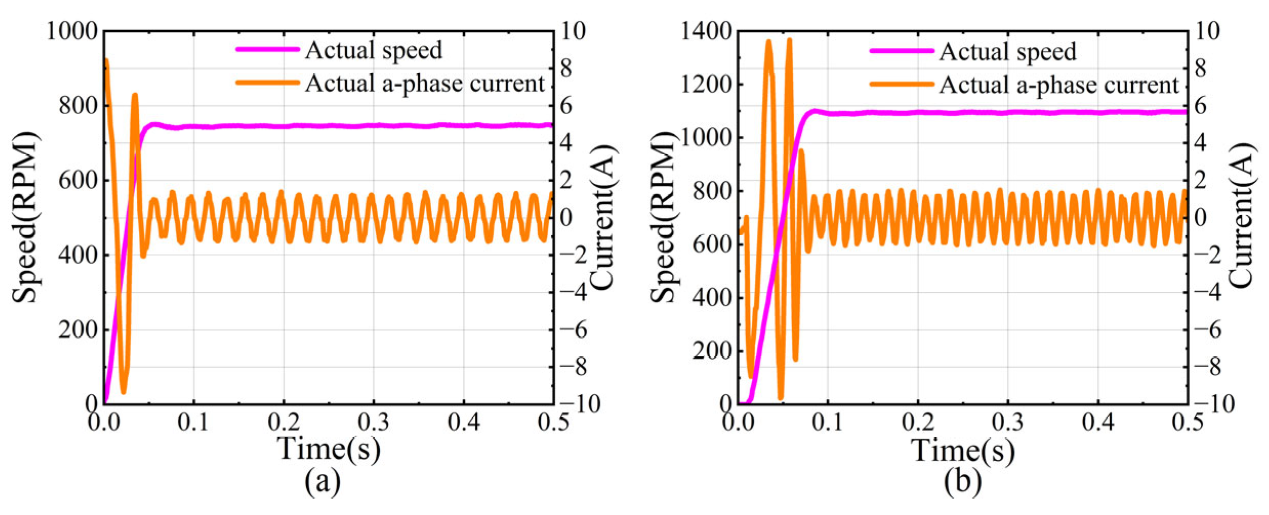
, which subsequently leads to an increase in motor current. Additionally, as the CFR decreases, the current continues to rise. To validate this phenomenon, the system’s sampling frequency was set to 15 kHz, and no-load experiments were conducted at speeds of 750 RPM and 1100 RPM. The results are presented in
Figure 10. Due to the adequately high sampling frequency, the delay of the control system at these two rotational speeds is only 1.2° and 1.8°, respectively.
As shown in
Figure 10, the current of the motor at both speeds is approximately 1.25 A. Due to the relatively small system delay, the current changes at these two speeds are not obvious. Moreover, under this experimental condition, when the speed reaches 1100 RPM, the
is 7 V. According to Equation (35), since:
it can be concluded that in the no-load experiment, the phenomenon of higher current is primarily attributed to the control delay caused by a relatively low CFR.
5. Discussion
In this paper, firstly, according to the characteristics of the low CFR of high-speed PMSM, a method for creating an accurate discrete mathematical model of SPMSM is proposed, and the accurate discrete mathematical model of SPMSM is established. Based on this model, a Luenberger observer suitable for low CFR systems is designed, and the position compensation under low CFR is provided. The experiments demonstrate that the ALO exhibits superior position estimation accuracy compared to that of the TLO at both high and low CFR. At CFRs of 30, 18, and 12.27, the RMS of the position errors of the ALO is only 20%, 12.4%, and 10.7% of those of the TLO, respectively, with the advantages of the ALO becoming more pronounced at lower CFRs. Furthermore, under conditions of varying speeds and abrupt load fluctuations, the position estimation accuracy achieved by the ALO demonstrates a consistent superiority compared to that of the TLO. This advantage stems from the position compensation in the accurate discrete motor model, which compensates for the effects of motor speed and sampling frequency on position estimation. This indicates that designing observers using the accurate discrete motor model is beneficial to improving observer accuracy.
The method for discretizing the mathematical model proposed in this paper is suitable for SPMSM. When applied to interior PMSMs, the complexity of its continuous time-domain mathematical model, along with the coupling between the α-axis and β-axis, leads to increased complexity in the derivation of its discrete mathematical representation. Additionally, the assumption that the motor speed remains constant within one sampling period may lead to significant position errors when the ALO is used in control systems requiring rapid speed changes and a high dynamic response. In the future, discrete modeling will take into account the angular acceleration of the motor to improve the accuracy of the observer’s observations. Meanwhile, in future work, the experiments will be conducted under the actual high-speed PMSMs operating conditions, with a sampling frequency of 10 KHz and a rotational speed ranging from 20,000 RPM to 50,000 RPM. Additionally, a comprehensive investigation will be carried out to analyze the stability of the observer in the presence of parameter uncertainty or fast dynamics.


