Mutual Information-Oriented ISAC Beamforming Design for Large Dimensional Antenna Array

Abstract

In this paper, we study the beamforming design for multiple-input multiple-output (MIMO) ISAC systems, with the weighted mutual information (MI) comprising sensing and communication perspectives adopted as the performance metric. In particular, the weighted sum of the communication mutual information and the sensing mutual information is shown to asymptotically converge to a deterministic limit when the number of transmitting and receiving antennas grow to infinity. This deterministic limit is derived by utilizing the operator-valued free probability theory. Subsequently, an efficient projected gradient ascent (PGA) algorithm is proposed to optimize the transmit beamforming matrix with the aim of maximizing the weighted asymptotic MI. Numerical results validate that the derived closed-form expression matches well with the Monte Carlo simulation results and the proposed optimization algorithm is able to improve the weighted asymptotic MI significantly. We also illustrate the trade-off between asymptotic sensing and asymptotic communication MI.

1. Introduction

The fifth generation (5G) wireless network has enabled numerous innovative applications, including smart cities and intelligent transportation systems. This technological advancement has consequently elevated the requirements for both communication and sensing capabilities across network nodes. Integrated sensing and communication (ISAC), which facilitates simultaneous information transmission and target sensing using shared wireless resources, has emerged as a crucial technology for future network implementation [1].

As a promising approach to enhance the performances of ISAC systems, beamforming design has been investigated in numerous works adopting various communication and sensing performance metrics. In [2], the authors considered transmit beampattern and signal-to-interference-plus-noise (SINR) as sensing and communication performance metrics, respectively. Furthermore, due to its capability of characterizing the lower bound of parameter estimation, the Cramér–Rao Bound (CRB) has also been adopted as a sensing performance metric in ISAC systems. In [3], the authors proposed an optimization framework for the CRB of radar sensing, under both point and extended target scenarios, while satisfying communication SINR constraints. In contrast, the authors in [4] maximized the achievable sum rate of the communication users under CRB constraint. To reduce the practical hardware cost, the authors in [5] investigated the partially connected hybrid beamforming design for ISAC systems, where the CRB for direct of arrival (DOA) estimation was minimized subject to the SINR constraints for communication users.

In most existing works, the performance metrics for sensing and communications are diverse, resulting in difficulties in evaluating the trade-offs between sensing and communication performance. To facilitate ISAC beamforming design under a unified performance metric, the authors in [6] proposed a Kullback–Leibler (KL) divergence-based unified performance metric, and analyzed the error rate performance of communication users and detection performance for sensing targets. Based on this unified metric, the authors in [7] investigated constellation and beamforming design, and depicted the Pareto bound in terms of KL divergence as well as bit error rate and detection probability. Different from KL divergence, which concentrates on the reliability of data transmission, mutual information (MI) is closely related to the efficiency of transmission, and has also been utilized as the performance metric in ISAC systems. Focusing on the sensing MI, the authors in [8] maximized the MI between the target response matrix of a point radar target under the data rate constraints of the communication users. As a step further, in [9], the authors derived the upper and lower bounds of both communication and sensing MI, and maximized the weighted MI. However, it should be noted that the aforementioned MI-oriented works were not conducted within the context of large dimensional antenna array, in which case perfect instantaneous channel state information (CSI) becomes challenging to obtain, thereby affecting the accuracy of MI. Compared to instantaneous CSI, statistical CSI can be more reliably acquired. In [10], the authors jointly designed the communication beamforming matrix and radar beampattern matrix in a MIMO radar and MIMO communication co-existence system with only statistical CSI. However, the ISAC beamforming design based on long-term channel statistics remains an open problem.

To address this issue, in this paper, we investigate the MI-oriented transmit beamforming design for a multiple-input multiple-output (MIMO) ISAC system, where ISAC user equipment (UE) senses an extended target while simultaneously transmitting data to a base station (BS). Based on the statistical CSI available at the UE, we formulate a transmit beamforming design problem with the aim of maximizing the weighted asymptotic MI. Applying the operator-valued free probability theory, we derive the closed-form expression of the weighted asymptotic MI and reformulate the beamforming design problem. Subsequently, based on the obtained closed-form expression, we propose an efficient projected gradient ascent (PGA) algorithm to solve the problem. Numerical results validate the accuracy of the derived expression, as well as the convergence and effectiveness of the proposed algorithm. In addition, the trade-off between sensing and communication MI is also depicted.

The remainder of this paper is organized as follows: Section 2 introduces the signal model and channel model, and formulates the transmit beamforming problem. In Section 3, we reformulate the optimization problem and propose the PGA algorithm. Then, simulation results are presented in Section 4. Finally, Section 5 concludes this paper.

2. System Model

2.1. Signal Model

We consider an ISAC system as shown in Figure 1, where an ISAC UE is physically equipped with $N_t$ transmitting antennas. The ISAC UE transmits data to the BS equipped with $N_u$ receiving antennas. Simultaneously, the transmitted signals impinge an extended target with L scatterers uniformly distributed in the proximity of the center. The echo signals are received by a sensing node equipped with $N_r$ antennas. The antennas at UE, BS, and the sensing node are assumed to be large dimensional antenna array (our results are still valid when the number of antennas is limited, which can be verified in the simulation results in Section 4). The transmit beamforming matrix of the UE is $\mathbf{W}\in {\mathbb{C}}^{N_t\times M}$. The  data symbol matrix is denoted as $\mathbf{S}\in {\mathbb{C}}^{M\times N_s}$, where $N_s$ denotes the number of signal samples and M denotes the number of data steams satisfying $M\le N_t$. It is assumed that the signal vectors of $\mathbf{S}$ are statistically orthogonal to each other, i.e., $\mathbb{E}\left[\mathbf{S}{\mathbf{S}}^{†}\right]={\mathbf{I}}_M$, with the notation ${(·)}^{†}$ denoting the conjugate transpose operation.

The received signal at BS can be expressed as

$$\begin{array}{c}\hfill {\mathbf{Y}}_c={\mathbf{H}}_c\mathbf{WS}+{\mathbf{N}}_C,\end{array}$$

(1)

where ${\mathbf{H}}_c$ is the channel between UE and BS, ${\mathbf{N}}_C=[{\mathbf{n}}_{c,1},\dots ,{\mathbf{n}}_{c,N_s}]\in {\mathbb{C}}^{N_u\times N_s}$ is the additive white Gaussian noise (AWGN) at the receiving antennas of BS, and ${\mathbf{n}}_{c,i}\sim \mathcal{CN}(0,{\sigma }_c^2{\mathbf{I}}_{N_u})$. The received echoes at the sensing node, ${\mathbf{Y}}_s\in {\mathbb{C}}^{N_r}$, can be expressed as

$$\begin{array}{c}\hfill {\mathbf{Y}}_s=\sum _{l=1}^L{\mathbf{G}}_l\mathbf{WS}+{\mathbf{N}}_S,\end{array}$$

(2)

where ${\mathbf{G}}_l\in {\mathbb{C}}^{N_r\times N_t}$ is the round-trip channel matrix between the $l-$th scatter and the sensing node, ${\mathbf{N}}_S=[{\mathbf{n}}_{s,1},\dots ,{\mathbf{n}}_{s,N_s}]\in {\mathbb{C}}^{N_r\times N_s}$ is the AWGN at the receiving antennas of the sensing node, and ${\mathbf{n}}_{s,i}\sim \mathcal{CN}(0,{\sigma }_s^2{\mathbf{I}}_{N_r})$.

2.2. Channel Model

We adopt the Weichselberger MIMO channel model [11] for both the radar sensing and communication channels, which comprehensively captures spatial correlations at both link ends along with their mutual coupling. Specifically, the channels in (1) and (2) can be expressed as

$$\begin{array}{cc}\hfill {\mathbf{H}}_c& ={\overline{\mathbf{H}}}_c+{\tilde{\mathbf{H}}}_c={\overline{\mathbf{H}}}_c+\mathbf{U}(\mathbf{M}\odot \mathbf{P}){\mathbf{V}}^{†},\hfill \end{array}$$

(3)

$$\begin{array}{cc}\hfill {\mathbf{G}}_l& ={\overline{\mathbf{G}}}_l+{\tilde{\mathbf{G}}}_l={\overline{\mathbf{G}}}_l+{\mathbf{R}}_l({\mathbf{N}}_l\odot {\mathbf{Q}}_l){\mathbf{T}}_l^{†},1\le l\le L,\hfill \end{array}$$

(4)

where ${\overline{\mathbf{H}}}_c$ and ${\overline{\mathbf{G}}}_l$ are deterministic matrices which denote the line-of-sight (LoS) component of ${\mathbf{H}}_c$ and ${\mathbf{G}}_l$, while ${\tilde{\mathbf{H}}}_c$ and ${\tilde{\mathbf{G}}}_l$ are the non-line-of-sight (NLoS) components of Hc and Gl, which contain the random variables. $\mathbf{U}$, $\mathbf{V}$, ${\mathbf{R}}_l$, and ${\mathbf{T}}_l$ are deterministic unitary matrices. $\mathbf{M}$ and ${\mathbf{N}}_l$ are deterministic nonnegative matrices which represent the variance profiles of the random components ${\tilde{\mathbf{H}}}_c$ and ${\tilde{\mathbf{G}}}_l$, respectively. $\mathbf{P}\in {\mathbb{C}}^{N_u\times N_t}$ and ${\mathbf{Q}}_l\in {\mathbb{C}}^{N_r\times N_t}$ are complex Gaussian distributed with ${\left[\mathbf{P}\right]}_{i,j}\sim \mathcal{CN}(0,1/N_t)$ and ${\left[{\mathbf{Q}}_l\right]}_{i,j}\sim \mathcal{CN}(0,1/N_t)$. In addition, the considered Weichselberger model can be degenerated to the Kronecker channel model by properly setting the matrics $\mathbf{U}$, $\mathbf{M}$, and $\mathbf{V}$.

Remark 1.

In this paper, we assume that the UE has access to accurate statistical CSI. This assumption is motivated by the fact that, as discussed in [10], statistical CSI varies slowly over time and can be more reliably acquired compared to instantaneous CSI. Therefore, it provides a practical basis for long-term system design. Nevertheless, we acknowledge that estimation errors in statistical CSI may arise in real-world scenarios. Investigating the impact of such imperfections on mutual information and beamforming performance constitutes an important direction for future work.

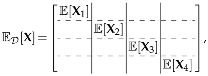
2.3. Problem Formulation

To facilitate the derivation of sensing MI, we assume that the receiving antennas of the sensing node form a sparsely spaced array with sufficiently large intervals, thereby making the spatial correlation among the receiving antennas negligible. Additionally, it is assumed that the scattering clusters in the sensing channel are primarily concentrated near the transmitter. Under these specific conditions, the sensing channel degenerates into a Kronecker channel, where ${\mathbf{R}}_l=\mathbf{I}$ in (4), and ${\mathbf{N}}_l$ can be expressed as the outer product of two vectors. From now on, for convenience of expression, we use ${\tilde{I}}_s\left({\sigma }^2\right)$ and ${\tilde{I}}_c\left({\sigma }^2\right)$ to denote ${\tilde{I}}_s\left({{\sigma }_s}^2\right)$ and ${\tilde{I}}_c\left({{\sigma }_c}^2\right)$, respectively. According to [12], the sensing MI can be expressed as

$$\begin{array}{cc}\hfill \widetilde{I_s}\left({\sigma }^2\right)& =\log \det \left({\mathbf{I}}_{N_s}+{\displaystyle \frac{1}{{\sigma }^2}}\sum _{l=1}^L\left({\mathbf{S}}^{†}{\mathbf{W}}^{†}{\mathbf{G}}_l^{†}{\mathbf{G}}_l\mathbf{WS}\right)\right)\hfill \\ \hfill & =\log \det \left({\mathbf{I}}_{L{N}_r}+{\displaystyle \frac{1}{{\sigma }^2}}\left(\widehat{\mathbf{G}}\mathbf{S}{\mathbf{S}}^{†}{\widehat{\mathbf{G}}}^{†}\right)\right),\hfill \end{array}$$

(5)

where the notation det$\left(\mathbf{A}\right)$ represents the determinant of matrix $\mathbf{A}$, and  the matrix $\widehat{\mathbf{G}}$ is defined as $\widehat{\mathbf{G}}={\left[{(\mathbf{G}}_1\mathbf{W}\right)}^{†},{(\mathbf{G}}_2{\mathbf{W})}^{†},\dots ,{(\mathbf{G}}_l\mathbf{W}{{)}^{†}]}^{†}$. Based on the received signal at BS, the communication MI for the considered ISAC system can be expressed as [13]

$$\begin{array}{cc}\hfill {\tilde{I}}_c\left({\sigma }^2\right)& =\log \det ({\mathbf{I}}_{N_u}+{\displaystyle \frac{1}{{\sigma }^2}}{\mathbf{H}}_c\mathbf{Q}{\mathbf{H}}_c^{†}),\hfill \end{array}$$

(6)

where $\mathbf{Q}=\mathbf{W}{\mathbf{W}}^{†}$. In order to achieve a balance between communication performance and sensing performance, we define a weighted MI as the performance metric for the proposed ISAC system, which is expressed as

$$\begin{array}{c}\hfill \tilde{I}\left(\mathbf{W}\right)=\rho {\tilde{I}}_s\left({\sigma }^2\right)+(1-\rho ){\tilde{I}}_c\left({\sigma }^2\right),\end{array}$$

(7)

where $\rho$ is a weighting factor that determines the weights of communication performance and sensing performance in the ISAC system. Furthermore, the transmit beamforming problem can be formulated as

$$\begin{array}{cc}\hfill \left(\mathbf{P}\mathbf{1}\right)& \underset{\mathbf{W}}{max}\tilde{I}\left(\mathbf{W}\right)\hfill \end{array}$$

(8a)

$$\begin{array}{c}\hfill \mathrm{s}.\mathrm{t}.{{∥\mathbf{W}∥}_F}^2\le P_t,\end{array}$$

(8b)

where ${∥·∥}_F$ denotes the Frobenius norm, (8b) is the transmit power constraint, and $P_t$ is the transmit power budget.

According to [14] (Thm. 2), for the sensing MI in (5) and communication MI in (6), we have

$$\begin{array}{cc}\hfill & {\displaystyle \frac{1}{L{N}_r}}\widetilde{I_s}\left({\sigma }^2\right)\underset{L{N}_r\to \infty }{\overset{a.s.}{\to }}{I}_s\left({\sigma }^2\right)\hfill \end{array}$$

(9)

$$\begin{array}{cc}\hfill & {\displaystyle \frac{1}{N_u}}\widetilde{I_c}\left({\sigma }^2\right)\underset{N_u\to \infty }{\overset{a.s.}{\to }}{I}_c\left({\sigma }^2\right)\hfill \end{array}$$

(10)

where the notation $\underset{L{N}_r\to \infty }{\overset{a.s.}{\to }}$ denotes the almost sure convergence as $L{N}_r$ and $N_t$ tend to infinity with the ratio $L{N}_r/N_t$ fixed. Similarly, $\underset{N_u\to \infty }{\overset{a.s.}{\to }}$ denotes the almost sure convergence as $N_u$ and $N_t$ tend to infinity with the ratio $N_u/N_t$ fixed. $I_s\left({\sigma }^2\right)$ and $I_c\left({\sigma }^2\right)$ are both deterministic, depending on the statistics of ${\mathbf{G}}_l$ and ${\mathbf{H}}_c$, respectively. However, since the channel statistics are not perfectly known at UE, we aim to optimize the weighted asymptotic MI, which is defined as

$$\begin{array}{c}\hfill I\left(\mathbf{W}\right)=\rho L{N}_r{I}_s\left({\sigma }^2\right)+(1-\rho )N_u{I}_c\left({\sigma }^2\right),\end{array}$$

(11)

Furthermore, the corresponding transmit beamforming problem can be formulated as follows:

$$\begin{array}{cc}\hfill \left(\mathbf{P}\mathbf{2}\right)& \underset{\mathbf{W}}{max}I\left(\mathbf{W}\right)\hfill \end{array}$$

(12a)

$$\begin{array}{c}\hfill \mathrm{s}.\mathrm{t}.{{∥\mathbf{W}∥}_F}^2\le P_t.\end{array}$$

(12b)

To solve this problem, we will derive the closed-form expression for the weighted asymptotic MI $I\left(\mathbf{W}\right)$ in Section 3.

3. Problem Reformulation and Proposed Algorithm

In this section, we reformulate Problem $\left(\mathbf{P}\mathbf{1}\right)$ and propose an efficient algorithm to solve the reformulated problem. Specifically, in Section 3.1, we first utilize the free probability theory and the linearization trick to derive the closed-form expression of the Cauchy transform. Based on this, we reformulate Problem $\left(\mathbf{P}\mathbf{1}\right)$ by deriving the closed-form expression for the weighted MI of the considered ISAC system. Finally, the PGA algorithm is proposed to solve the reformulated problem in Section 3.2.

3.1. Problem Reformulation

Denote ${\mathbf{B}}_1=\widehat{\mathbf{G}}\mathbf{S}{\mathbf{S}}^{†}{\widehat{\mathbf{G}}}^{†}$ and define the empirical cumulative distribution function (ECDF) of the ${\mathbf{B}}_1$’s eigenvalues as

$$\begin{array}{c}\hfill {\tilde{F}}_{{\mathbf{B}}_1}\left(x\right)={\displaystyle \frac{1}{L{N}_r}}\sum _{i=1}^{L{N}_r}1\{{\lambda }_i\left({\mathbf{B}}_1\right)\le x\},\end{array}$$

(13)

where ${\lambda }_1\left({\mathbf{B}}_1\right)$,…,${\lambda }_{L{N}_r}\left({\mathbf{B}}_1\right)$ are the eigenvalues of ${\mathbf{B}}_1$, $1\{·\}$ is the indicator function, and $1\{{\lambda }_i\left({\mathbf{B}}_1\right)\le x\}=\left\{\begin{array}{c}1,if{\lambda }_i\left({\mathbf{B}}_1\right)\le x\\ 0,otherwise\end{array}\right\}$. Therefore, ${\displaystyle \frac{1}{L{N}_r}}{\tilde{I}}_s\left({\sigma }^2\right)$ can be rewritten as

$$\begin{array}{cc}\hfill {\displaystyle \frac{1}{L{N}_r}}{\tilde{I}}_s\left({\sigma }^2\right)& ={\displaystyle \frac{1}{L{N}_r}}\log \det \left({\mathbf{I}}_{L{N}_r}+{\displaystyle \frac{1}{{\sigma }^2}}{\mathbf{B}}_1\right),\hfill \\ \hfill & =\sum _{i=1}^{L{N}_r}log\left(1+{\displaystyle \frac{1}{{\sigma }^2}}{\lambda }_i\left({\mathbf{B}}_1\right)\right),\hfill \\ \hfill & ={\int }_0^{\infty }log(1+{\displaystyle \frac{1}{{\sigma }^2}}x)d{\tilde{F}}_{{\mathbf{B}}_1}\left(x\right).\hfill \end{array}$$

(14)

For ${\mathbf{B}}_1$, its resolvent ${\tilde{\mathcal{G}}}_{{\mathbf{B}}_1}(-z)$ and Cauchy transform ${\mathcal{G}}_{{\mathbf{B}}_1}(-z)$ for ${\mathbf{B}}_1$ are defined as

$$\begin{array}{c}\hfill {\tilde{\mathcal{G}}}_{{\mathbf{B}}_1}\left(z\right)={\displaystyle \frac{1}{L{N}_r}}\mathrm{Tr}{(z\mathbf{I}-{\mathbf{B}}_1)}^{-1}={\int }_0^{\infty }{\displaystyle \frac{1}{z-\lambda }}\mathrm{d}{\tilde{F}}_{{\mathbf{B}}_1},\end{array}$$

(15)

$$\begin{array}{c}\hfill {\mathcal{G}}_{{\mathbf{B}}_1}\left(z\right)={\displaystyle \frac{1}{L{N}_r}}\mathbb{E}\left[\mathrm{Tr}{(z\mathbf{I}-{\mathbf{B}}_1)}^{-1}\right]={\int }_0^{\infty }{\displaystyle \frac{1}{z-\lambda }}\mathrm{d}{F}_{{\mathbf{B}}_1}.\end{array}$$

(16)

where $z=-{\displaystyle \frac{1}{{\sigma }^2}}$ and $F_{{\mathbf{B}}_1}$ is the cumulative distribution function (CDF) of the eigenvalues of ${\mathbf{B}}_1$. Therefore, we have

$$\begin{array}{c}\hfill {\displaystyle \frac{1}{L{N}_r}}{\displaystyle \frac{d{\tilde{I}}_s\left({\sigma }^2\right)}{dz}}=-{\displaystyle \frac{1}{z}}-{\tilde{\mathcal{G}}}_{{\mathbf{B}}_1}(-z).\end{array}$$

(17)

Applying the relationship between the Shannon transform ${\mathcal{V}}_{{\mathbf{B}}_1}\left(z\right)$ and the Cauchy transform ${\mathcal{G}}_{{\mathbf{B}}_1}(-z)$, the following equation holds

$$\begin{array}{c}\hfill {\displaystyle \frac{d{\mathcal{V}}_{{\mathbf{B}}_1}\left(z\right)}{dz}}=-{\displaystyle \frac{1}{z}}-{\mathcal{G}}_{{\mathbf{B}}_1}(-z).\end{array}$$

(18)

According to [15], the resolvent ${\tilde{\mathcal{G}}}_{{\mathbf{B}}_1}(-z)$ converges almost surely to the Cauchy transform ${\mathcal{G}}_{{\mathbf{B}}_1}(-z)$ for ${\mathbf{B}}_1$. Therefore, we have

$$\begin{array}{c}\hfill {\displaystyle \frac{1}{L{N}_r}}\widetilde{I_s}\left({\sigma }^2\right)\underset{L{N}_r\to \infty }{\overset{a.s.}{\to }}{\mathcal{V}}_{{\mathbf{B}}_1}\left(z\right).\end{array}$$

(19)

Since (9) holds, we can rewrite $I_s\left({\sigma }^2\right)$ as

$$\begin{array}{c}\hfill I_s\left({\sigma }^2\right)={\mathcal{V}}_{{\mathbf{B}}_1}\left(z\right).\end{array}$$

(20)

Similarly, for the asymptotic communication MI, we have

$$\begin{array}{ll}\hfill & I_c\left({\sigma }^2\right)={\mathcal{V}}_{{\mathbf{B}}_2}\left(z\right),\hfill \end{array}$$

(21)

$$\begin{array}{ll}\hfill & {\displaystyle \frac{d{\mathcal{V}}_{{\mathbf{B}}_2}\left(z\right)}{dz}}=-{\displaystyle \frac{1}{z}}-{\mathcal{G}}_{{\mathbf{B}}_2}(-z),\hfill \end{array}$$

(22)

$$\begin{array}{cc}\hfill & {\mathcal{G}}_{{\mathbf{B}}_2}\left(z\right)={\int }_0^{\infty }{\displaystyle \frac{1}{z-\lambda }}\mathrm{d}{F}_{{\mathbf{B}}_2}\left(\lambda \right)\hfill \end{array}$$

(23)

where ${\mathbf{B}}_2={\mathbf{H}}_c\mathbf{Q}{\mathbf{H}}_c^{†}$, $F_{{\mathbf{B}}_{\mathbf{2}}}\left(\lambda \right)$ is CDF of ${\mathbf{B}}_2$, ${\mathcal{V}}_{{\mathbf{B}}_2}\left({\sigma }^2\right)$ is the Shannon transform of ${\mathbf{B}}_2$, and ${\mathcal{G}}_{{\mathbf{B}}_2}\left(z\right)$ is the Cauchy transform of ${\mathbf{B}}_2$.

To obtain the closed-form expression of ${\mathcal{G}}_{{\mathbf{B}}_i}\left(z\right)$, free probability theory serves as a powerful analytical tool [16]. However, in the considered system, $\widehat{\mathbf{G}}$ and $\mathbf{S}$ are not free in the classic free probability aspect, resulting in difficulties in directly obtaining the Cauchy Transform for the products of $\widehat{\mathbf{G}}$, $\mathbf{S}$, ${\mathbf{S}}^{†}$, and ${\widehat{\mathbf{G}}}^{†}$[17]. To address this issue, we employ a linearization trick to embed the non-free matrices into a higher-dimensional matrix. Within this framework, the deterministic and random components are shown to exhibit asymptotic freeness. Consequently, the target Cauchy transform can be derived by transforming the operator-valued Cauchy transform of the embedded matrix. For the convenience of expression, we define $\overline{\mathbf{G}}={\left[{(\overline{\mathbf{G}}}_1\mathbf{W}\right)}^T,{\left({\overline{\mathbf{G}}}_2\mathbf{W}\right)}^T,\dots ,{{\left({\overline{\mathbf{G}}}_l\mathbf{W}\right)}^T]}^T$, and $\overline{\mathbf{H}}={\overline{\mathbf{H}}}_c\mathbf{W}$. Since $I_c$ and $I_s$ share a similar form, we only provide the detailed derivation of ${\mathcal{G}}_{{\mathbf{B}}_1}\left(z\right)$.

To obtain the closed-form of ${\mathcal{G}}_{{\mathbf{B}}_1}\left(z\right)$, we first introduce the following Multiplicative Linearization trick [16].

Lemma 1

(Multiplicative Linearization). The product of matrices $\mathbf{Z}={\mathbf{X}}_1{\mathbf{X}}_2\dots {\mathbf{X}}_M\in {\mathbb{C}}^{n\times n}$ can be linearized as

$${\mathbf{Z}}_l=\left[\begin{array}{cccc}\hfill & \hfill & & {\mathbf{X}}_1\hfill \\ \hfill & \hfill & {\mathbf{X}}_2\hfill & -\mathbf{I}\hfill \\ \hfill & ⋰\hfill & ⋰\hfill \\ {\mathbf{X}}_M\hfill & -\mathbf{I}\hfill & \hfill \end{array}\right]$$

(24)

The operator-valued Cauchy transforms of the matrix $\mathbf{Z}$ and the corresponding linearized matrix ${\mathbf{Z}}_l$ are related as follows

$${\mathcal{G}}_{\mathbf{Z}}^{\mathcal{D}}\left(z\right)={\left({\mathcal{G}}_{{\mathbf{Z}}_l}^{\mathcal{D}}(\mathbf{\Gamma }\left(z\right))\right)}^{\left(n\right)},$$

(25)

where the matrix $\Gamma \left(z\right)$ is given by

$$\mathbf{\Gamma }\left(z\right)=\left[\begin{array}{cc}z{\mathbf{I}}_n& \mathbf{0}\\ \mathbf{0}& \mathbf{0}\end{array}\right].$$

(26)

Proof. 

The detailed proof of Lemma 1 can be found in [16].    □

By applying Lemma 1, the linearized block matrix of ${\mathbf{B}}_1=\widehat{\mathbf{G}}\mathbf{S}{\mathbf{S}}^{†}{\widehat{\mathbf{G}}}^{†}$, with the size of $(L{N}_r+N_s+2M)\times (L{N}_r+N_s+2M)$, can be constructed as

$$\begin{array}{c}\hfill {\mathbf{B}}_L=\left[\begin{array}{cccc}{\mathbf{0}}_{L{N}_r\times L{N}_r}& {\mathbf{0}}_{L{N}_r\times M}& {\mathbf{0}}_{L{N}_r\times N_s}& \widehat{\mathbf{G}}\\ {\mathbf{0}}_{M\times L{N}_r}& {\mathbf{0}}_{M\times M}& \mathbf{S}& -{\mathbf{I}}_M\\ {\mathbf{0}}_{N_s\times L{N}_r}& {\mathbf{S}}^{†}& -{\mathbf{I}}_{N_s}& {\mathbf{0}}_{N_s\times M}\\ {\widehat{\mathbf{G}}}^{†}& -{\mathbf{I}}_M& {\mathbf{0}}_{M\times N_s}& {\mathbf{0}}_{M\times M}\end{array}\right].\end{array}$$

(27)

The operator-valued Cauchy transform ${\mathcal{G}}_{{\mathbf{B}}_L}^{\mathcal{D}}$ [16] is given by

$$\begin{array}{c}\hfill {\mathcal{G}}_{{\mathbf{B}}_L}^{\mathcal{D}}(\mathbf{\Gamma }\left(z\right))={\mathbb{E}}_{\mathcal{D}}\left[{\left(\mathbf{\Gamma }\left(z\right)-{\mathbf{B}}_L\right)}^{-1}\right],\end{array}$$

(28)

where ${\mathbb{E}}_{\mathcal{D}}\left[\mathbf{X}\right]$ is defined as

(29)

where ${\mathbf{X}}_1={\left\{\mathbf{X}\right\}}_1^{L{N}_r}$, ${\mathbf{X}}_2={\left\{\mathbf{X}\right\}}_{L{N}_r+1}^{L{N}_r+M}$, ${\mathbf{X}}_3={\left\{\mathbf{X}\right\}}_{L{N}_r+M+1}^{L{N}_r+M+N_s}$, and ${\mathbf{X}}_4={\left\{\mathbf{X}\right\}}_{L{N}_r+M+N_s+1}^{L{N}_r+2M+N_s}$, with ${\left\{\mathbf{A}\right\}}_a^b$ denoting the submatrix of $\mathbf{A}$ from indices a to b, i.e.,  ${\left[{\left\{\mathbf{A}\right\}}_a^b\right]}_{i,j}={\left[\mathbf{A}\right]}_{i+a-1,j+a-1}$ for $1\le i,j\le b-a+1$, where ${\left[\mathbf{A}\right]}_{i,j}$ represents the element in the i-th row and j-th column of $\mathbf{A}$. In addition, the matrix $\mathbf{\Gamma }\left(z\right)$ is defined as

$$\begin{array}{c}\hfill \mathbf{\Gamma }\left(z\right)=\left[\begin{array}{cc}z{\mathbf{I}}_{L{N}_r}& {\mathbf{0}}_{L{N}_r\times (N_s+2M)}\\ {\mathbf{0}}_{(N_s+2M)\times L{N}_r}& {\mathbf{0}}_{(N_s+2M)\times (N_s+2M)}\end{array}\right].\end{array}$$

(30)

Then, ${\mathcal{G}}_{{\mathbf{B}}_1}\left(z\right)$ is given by

$$\begin{array}{c}\hfill {\mathcal{G}}_{{\mathbf{B}}_1}\left(z\right)={\displaystyle \frac{1}{L{N}_r}}\mathrm{Tr}\left({\left\{{\mathcal{G}}_{{\mathbf{B}}_L}^{\mathcal{D}}(\mathbf{\Gamma }\left(z\right))\right\}}^{(1,1)}\right),\end{array}$$

(31)

where ${\{·\}}^{(1,1)}$ represents the upper-left $L{N}_r\times L{N}_r$ block matrix and the operator $\mathrm{Tr}(·)$ represents the trace of the matrix. It can be observed that ${\mathbf{B}}_L$ shares a similar structure with the matrix $\mathbf{L}$ proposed in [18] (Prop. 2), which inspires us to use the method in [18]. Specifically, the  Cauchy transform ${\mathcal{G}}_{{\mathbf{B}}_1}\left(z\right)$ can be obtained with the following proposition.

Proposition 1.

The Cauchy transform of ${\mathbf{B}}_1$, with $z\in {\mathbb{C}}^{+}$, is given by

$$\begin{array}{c}\hfill {\mathcal{G}}_{{\mathbf{B}}_1}\left(z\right)={\displaystyle \frac{1}{L{N}_r}}\mathrm{Tr}\left[{\mathcal{G}}_{\tilde{\mathbf{C}}}\left(z\right)\right],\end{array}$$

(32)

where ${\mathcal{G}}_{\tilde{\mathbf{C}}}\left(z\right)$ satisfies

$$\begin{array}{cc}\hfill {\mathcal{G}}_{\tilde{\mathbf{C}}}\left(z\right)& ={\left(\tilde{\mathbf{\Psi }}\left(z\right)-\overline{\mathbf{G}}{\Pi }^{-1}{\overline{\mathbf{G}}}^{†}\right)}^{-1},\hfill \end{array}$$

(33)

$$\begin{array}{cc}\hfill \mathbf{\Pi }& =\mathbf{\Psi }\left(z\right)-\tilde{\mathbf{\Phi }}{\left(z\right)}^{-1},\hfill \end{array}$$

(34)

where the matrices $\tilde{\mathbf{\Psi }}\left(z\right)$, $\mathbf{\Psi }\left(z\right)$, $\tilde{\mathbf{\Phi }}\left(z\right)$, $\mathbf{\Phi }\left(z\right)$ are, respectively, denoted as

$$\begin{array}{ll}\tilde{\mathbf{\Psi }}\left(z\right)\hfill & =z{\mathbf{I}}_{L{N}_r}-\mathrm{diag}\left\{{\tilde{\eta }}_1\left({\mathcal{G}}_{\mathbf{C}}\left(z\right)\right),\dots ,{\tilde{\eta }}_L({\mathcal{G}}_{\mathbf{C}}\left(z\right)\right\},\hfill \end{array}$$

(35)

$$\begin{array}{cc}\hfill \mathbf{\Psi }\left(z\right)& =-\sum _{l=1}^L{\eta }_l\left({\mathcal{G}}_{{\tilde{\mathbf{C}}}_l}\left(z\right)\right),\hfill \end{array}$$

(36)

$$\begin{array}{cc}\hfill \tilde{\mathbf{\Phi }}\left(z\right)& =-\tilde{\zeta }\left({\mathcal{G}}_{\tilde{\mathbf{D}}}\left(z\right)\right),\hfill \end{array}$$

(37)

$$\begin{array}{cc}\hfill \mathbf{\Phi }\left(z\right)& ={\mathbf{I}}_{N_s}-\zeta \left({\mathcal{G}}_{\mathbf{D}}\left(z\right)\right),\hfill \end{array}$$

(38)

where the diag$({\mathbf{X}}_{\mathbf{1}},\dots ,{\mathbf{X}}_{\mathbf{n}})$ represents the diagonal block matrix constructed by the ${\mathbf{X}}_{\mathbf{1}},\dots ,{\mathbf{X}}_{\mathbf{n}}$ matrices and ${\eta }_l\left(\tilde{\mathbf{C}}\right)$, ${\tilde{\eta }}_l\left(\mathbf{C}\right)$, $\zeta \left(\mathbf{D}\right)$, $\tilde{\zeta }\left(\tilde{\mathbf{D}}\right)$ are the parameterized one-sided correlation matrices, which are shown as (A1), (A2), (A9), and (A10) in Appendix A. The matrices ${\mathcal{G}}_{\mathbf{C}}\left(z\right)$, ${\mathcal{G}}_{\tilde{\mathbf{D}}}\left(z\right)$, ${\mathcal{G}}_{\mathbf{D}}\left(z\right)$, and ${\mathcal{G}}_{{\tilde{\mathbf{C}}}_l}\left(z\right)$ are defined as

$$\begin{array}{cc}\hfill {\mathcal{G}}_{\mathbf{C}}\left(z\right)& ={\left(\mathbf{\Psi }\left(z\right)-{\overline{\mathbf{G}}}^{†}\tilde{\mathbf{\Psi }}{\left(z\right)}^{-1}{\overline{\mathbf{G}}}^{†}-\tilde{\mathbf{\Phi }}{\left(z\right)}^{-1}\right)}^{-1},\hfill \end{array}$$

(39)

$$\begin{array}{cc}\hfill {\mathcal{G}}_{\tilde{\mathbf{D}}}\left(z\right)& =\mathbf{\Phi }{\left(z\right)}^{-1},\hfill \end{array}$$

(40)

$$\begin{array}{cc}\hfill {\mathcal{G}}_{\mathbf{D}}\left(z\right)& ={\left(\tilde{\mathbf{\Phi }}\left(z\right)-{\left(\mathbf{\Psi }\left(z\right)-{\overline{\mathbf{G}}}^{†}\tilde{\mathbf{\Psi }}\left(z\right)\overline{\mathbf{G}}\right)}^{-1}\right)}^{-1},\hfill \end{array}$$

(41)

$$\begin{array}{cc}\hfill {\mathcal{G}}_{{\tilde{\mathbf{C}}}_l}\left(z\right)& ={\left\{{\mathcal{G}}_{\tilde{\mathbf{C}}}\left(z\right)\right\}}_{1+(l-1)N_r}^{l{N}_r}.\hfill \end{array}$$

(42)

Proof. 

The proof of this Proposition 1 is similar to the method presented in [18] (Prop. 2). Therefore we provide a brief outline of the proof. First, we prove that the deterministic and random components of the linearized matrix are free. Then, by applying the subordination formula, we derive the equation for the operator-valued Cauchy transform. Finally, using the matrix inversion formula, we decompose the operator-valued Cauchy transform, thereby obtaining the above expressions.    □

Based on the closed-form expression of the Cauchy transformation ${\mathcal{G}}_{{\mathbf{B}}_1}\left(z\right)$, we can obtain the closed-form expression of ${\mathcal{V}}_{{\mathbf{B}}_1}\left(z\right)$ via the following proposition.

Proposition 2.

The Shannon transform ${\mathcal{V}}_{{\mathbf{B}}_1}\left(z\right)$, with $z\in {\mathbb{C}}^{+}$, is given by

$$\begin{array}{cc}\hfill {\mathcal{V}}_{{\mathbf{B}}_1}\left(z\right)& ={\displaystyle \frac{1}{L{N}_r}}logdet\left({\displaystyle \frac{\tilde{\mathbf{\Psi }}\left(-z\right)}{-z}}\right)+{\displaystyle \frac{1}{L{N}_r}}logdet\left(\mathbf{\Psi }(-z)-{\overline{\mathbf{G}}}^{†}\tilde{\mathbf{\Psi }}{(-z)}^{-1}{\overline{\mathbf{G}}}^{†}-\tilde{\mathbf{\Phi }}{(-z)}^{-1}\right)\hfill \\ \hfill & +{\displaystyle \frac{1}{L{N}_r}}logdet\left(\tilde{\mathbf{\Phi }}(-z)\right)+{\displaystyle \frac{1}{L{N}_r}}\mathrm{Tr}\left({\mathcal{G}}_{\tilde{\mathbf{C}}}(-z)\left(-z{\mathbf{I}}_{LNr}-\tilde{\mathbf{\Psi }}(-z)\right)\right),\hfill \\ \hfill & +{\displaystyle \frac{1}{L{N}_r}}\mathrm{Tr}\left({\mathcal{G}}_{\tilde{\mathbf{D}}}(-z)\zeta \right)+{\displaystyle \frac{1}{L{N}_r}}logdet\left(\mathbf{\Phi }(-z)\right)\hfill \end{array}$$

(43)

where $\tilde{\mathbf{\Psi }}(-z)$, $\mathbf{\Psi }(-z)$, $\tilde{\mathbf{\Phi }}(-z)$, ${\mathcal{G}}_{\tilde{\mathbf{D}}}(-z)$, ${\mathcal{G}}_{\mathbf{D}}(-z)$, and ${\mathcal{G}}_{\tilde{\mathbf{C}}}\left(-z\right)$ are given by (33)–(38) in Proposition 1.

Proof. 

The proof of Propsition 2 is given in Appendix B.    □

Similarly, the Cauchy transform ${\mathcal{G}}_{{\mathbf{B}}_2}\left(z\right)$ of ${\mathbf{B}}_2$ and the Shannon transform ${\mathcal{V}}_{{\mathbf{B}}_2}\left(z\right)$ can be expressed by

$$\begin{array}{cc}\hfill {\mathcal{G}}_{{\mathbf{B}}_2}\left(z\right)& ={\displaystyle \frac{1}{N_u}}\mathrm{Tr}\left[{\mathcal{G}}_{\tilde{\mathbf{E}}}\left(z\right)\right],\hfill \end{array}$$

(44)

$$\begin{array}{cc}\hfill {\mathcal{V}}_{{\mathbf{B}}_2}\left(z\right)& ={\displaystyle \frac{1}{N_u}}logdet\left({\displaystyle \frac{\tilde{\mathbf{\Omega }}\left(-z\right)}{-z}}\right)+{\displaystyle \frac{1}{N_u}}\mathrm{Tr}\left({\mathcal{G}}_{\tilde{\mathbf{E}}}(-z)\tilde{\tau }\right)\hfill \\ \hfill & -{\displaystyle \frac{1}{N_u}}logdet\left({\mathcal{G}}_{\mathbf{E}}(-z)\right),\hfill \end{array}$$

(45)

where ${\eta }_l\left(\tilde{\mathbf{C}}\right)$, ${\tilde{\eta }}_l\left(\mathbf{C}\right)$, $\tau \left(\mathbf{E}\right)$, $\tilde{\tau }\left(\tilde{\mathbf{E}}\right)$ are the parameterized one-sided correlation matrices, which are shown as (A1), (A2), (A5), and (A6) in Appendix A. The matrices ${\mathcal{G}}_{\tilde{\mathbf{E}}}\left(z\right)$, ${\mathcal{G}}_{\mathbf{E}}\left(z\right)$, $\tilde{\mathbf{\Omega }}\left(z\right)$, and $\mathbf{\Omega }\left(z\right)$ satisfy the following equations

$$\begin{array}{cc}\hfill {\mathcal{G}}_{\tilde{\mathbf{E}}}\left(z\right)& ={\left(\tilde{\mathbf{\Omega }}\left(z\right)-\overline{\mathbf{H}}\mathbf{\Omega }{\left(z\right)}^{-1}{\overline{\mathbf{H}}}^{†}\right)}^{-1},\hfill \end{array}$$

(46)

$$\begin{array}{cc}\hfill {\mathcal{G}}_{\mathbf{E}}\left(z\right)& ={\left(\mathbf{\Omega }\left(z\right)-{\overline{\mathbf{H}}}^{†}\tilde{\mathbf{\Omega }}{\left(z\right)}^{-1}\overline{\mathbf{H}}\right)}^{-1},\hfill \end{array}$$

(47)

$$\begin{array}{cc}\hfill \tilde{\mathbf{\Omega }}\left(z\right)& =z{\mathbf{I}}_{N_u}-\tilde{\tau }\left({\mathcal{G}}_{\mathbf{E}}\left(z\right)\right),\hfill \end{array}$$

(48)

$$\begin{array}{cc}\hfill \mathbf{\Omega }\left(z\right)& ={\mathbf{I}}_{N_t}-\tau \left({\mathcal{G}}_{\tilde{\mathbf{E}}}\left(z\right)\right).\hfill \end{array}$$

(49)

From now on, for convenience of expression, we refer to the asymptotic sensing MI, asymptotic communication MI, and weighted asymptotic MI as the sensing MI, communication MI, and weighted MI, respectively. Then, the sensing MI, the communication MI and the weighted MI can be rewritten as

$$\begin{array}{cc}\hfill I_s({\sigma }^2,\mathbf{W})& =L{N}_r{\mathcal{V}}_{{\mathbf{B}}_1}\left({\sigma }^2\right),\hfill \end{array}$$

(50)

$$\begin{array}{cc}\hfill I_c({\sigma }^2,\mathbf{W})& =N_u{\mathcal{V}}_{{\mathbf{B}}_2}\left({\sigma }^2\right),\hfill \end{array}$$

(51)

$$\begin{array}{cc}\hfill I({\sigma }^2,\mathbf{W})& =\rho I_s({\sigma }^2,\mathbf{W})+(1-\rho )I_c({\sigma }^2,\mathbf{W}).\hfill \end{array}$$

(52)

Consequently, we reformulate the problem $\left(\mathbf{P}\mathbf{2}\right)$ as

$$\begin{array}{c}\hfill \left(\mathbf{P}\mathbf{3}\right) \underset{\mathbf{W}}{max}I({\sigma }^2,\mathbf{W})\end{array}$$

(53a)

$$\begin{array}{cc}& \mathrm{s}.\mathrm{t}.{{∥\mathbf{W}∥}_F}^2\le P_t,\hfill \end{array}$$

(53b)

3.2. Proposed PGA Algorithm

In order to solve the problem $\left(\mathbf{P}\mathbf{3}\right)$, we propose the PGA algorithm. Firstly, we calculate the gradient of the weighted MI in (52). Then, the updated beamforming matrix at the $(i+1)$-th iteration is updated as

$$\begin{array}{c}\hfill {\tilde{\mathbf{W}}}^{\left[i+1\right]}={\mathbf{W}}^{\left[i\right]}+\lambda \nabla g_{\mathbf{W}}\left({\mathbf{W}}^{\left[i\right]}\right),\end{array}$$

(54)

where ${\mathbf{W}}^{\left[i\right]}$ denotes the beamforming matrix at the i-th iteration, $\lambda$ denotes the step size, and the element of gradient $\nabla g_{\mathbf{W}}$ of $I(z,\mathbf{W})$ is given by  

$$\begin{array}{cc}\hfill {[\nabla g_{\mathbf{W}}]}_{i,j}=& \rho \mathrm{Tr}\left({\left(-\mathbf{\Psi }+{\mathbf{W}}^{†}\overline{\mathbf{G}}{\tilde{\mathbf{\Psi }}}^{-1}\overline{\mathbf{G}}\mathbf{W}+{\tilde{\mathbf{\Phi }}}^{-1}\right)}^{-1}{\mathbf{E}}_{i,j}^{†}{\overline{\mathbf{G}}}^{†}{\tilde{\mathbf{\Psi }}}^{-1}\overline{\mathbf{G}}\mathbf{W}\right)\hfill \\ \hfill & +(\rho -1)\mathrm{Tr}\left({\left(\mathbf{\Omega }-{\mathbf{W}}^{†}{\overline{\mathbf{H}}}^{†}{\tilde{\mathbf{\Omega }}}^{-1}\overline{\mathbf{H}}\mathbf{W}\right)}^{-1}{\mathbf{E}}_{i,j}^{†}{\overline{\mathbf{H}}}^{†}{\tilde{\mathbf{\Omega }}}^{-1}\overline{\mathbf{H}}\mathbf{W}\right),\hfill \end{array}$$

(55)

where ${\mathbf{E}}_{i,j}$ is a matrix whose elements satisfy

$$\begin{array}{c}\hfill {\left[{\mathbf{E}}_{i,j}\right]}_{s,t}=\left\{\begin{array}{c}1,\mathrm{if}s=i\mathrm{and}t=j,\\ 0,\mathrm{otherwise}.\end{array}\right.\end{array}$$

(56)

To satisfy the transmit power constraint (8b), the solution ${\tilde{\mathbf{W}}}^{\left[i+1\right]}$ is then projected onto the feasible region. The obtained solution at the $(i+1)$-th iteration is given by

$$\begin{array}{c}\hfill {\mathbf{W}}^{\left[i+1\right]}={\mathrm{Proj}}_W\left({\tilde{\mathbf{W}}}^{\left[i+1\right]}\right),\end{array}$$

(57)

where the projection operator is given as

$$\begin{array}{c}\hfill {\mathrm{Proj}}_W=\left\{\begin{array}{c}\mathbf{W},if{{∥\mathbf{W}∥}_F}^2\le P_t,\\ \sqrt{P_t}{\displaystyle \frac{\mathbf{W}}{{∥\mathbf{W}∥}_F}},otherwise.\end{array}\right.\end{array}$$

(58)

The detailed algorithm is presented in Algorithm 1. Specifically, in each iteration of the PGA algorithm, we first calculate the gradient of the beamforming matrix $\mathbf{W}$ with (55), and then update it with (54). The matrices in (55) are obtained by iteratively calculating fixed point Equations (35)–(38) and (46)–(49).

Algorithm 1 PGA algorithm for beamforming matrix design

initialize: Set $i=0$ and initialize the beamforming matrix ${\mathbf{W}}^{\left[0\right]}$. Calculate $I^{\left[0\right]}$ based on (52). repeat    Update ${\mathbf{W}}^{\left[i+1\right]}$ based on (57).    Calculate $I^{[i+1]}$ based on (52).    $i=i+1$. until $|I^{\left[i\right]}-I^{[i-1]}|\le \epsilon$. output Optimal beamforming matrix $\mathbf{W}$.

For the complexity analysis, it can be noted that the complexity of the proposed PGA algorithm mainly comes from the calculation of the matrices in (39)–(42) and (46)–(49). Assuming that the number of iterations of the fixed point equation in (39)–(42) and (46)–(49) are $I_1$ and $I_2$, the number of iterations for the PGA is $I_{out}$, and it only keeps the leading order terms, the complexity of the PGA algorithm is proportional to $O(I_{out}(I_1{\left(N_t\right)}^3+{(N_r+L)}^3)+I_2({\left(N_r\right)}^3+N_u^3)+{(N_r+L)}^3+N_u^3))$.

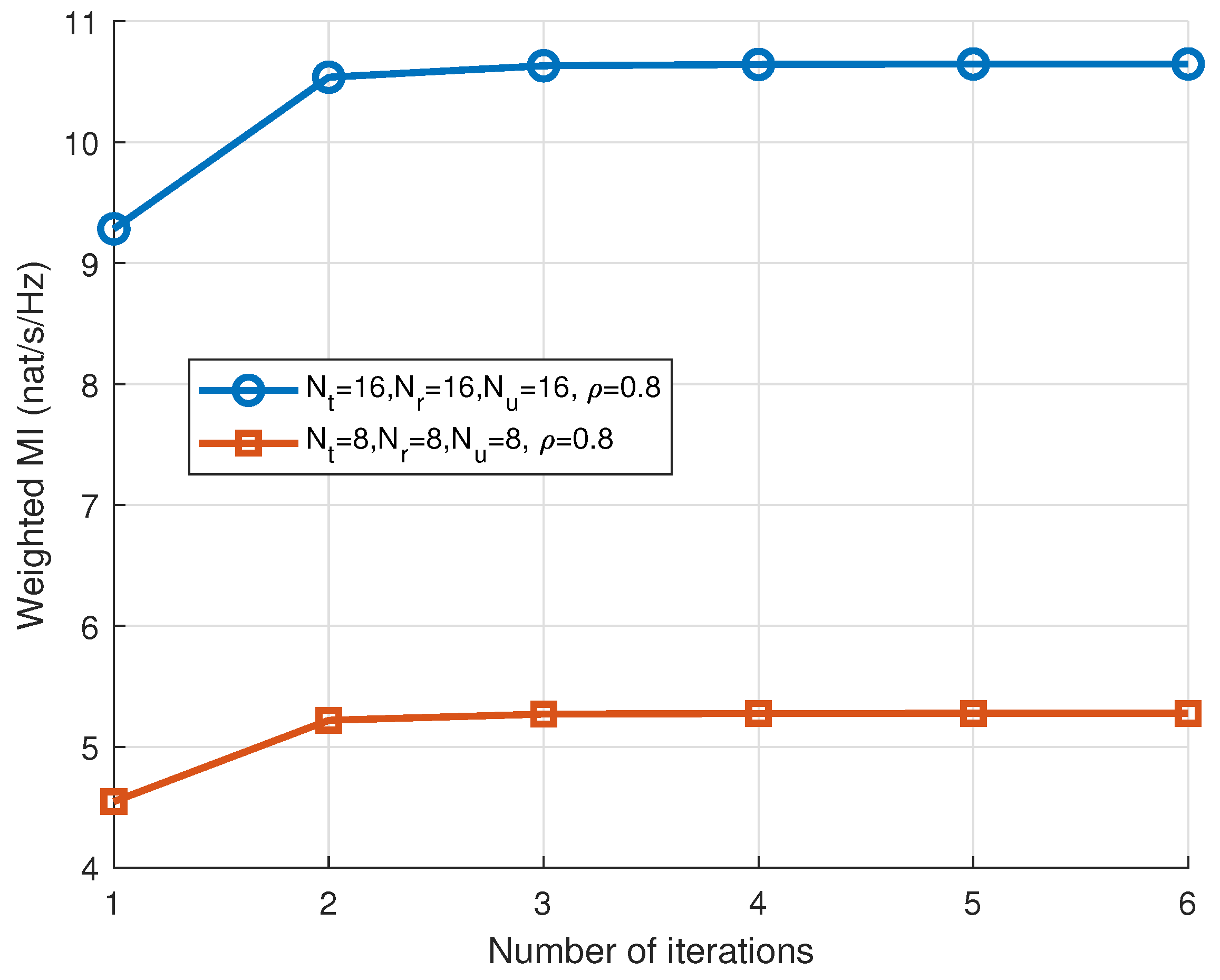
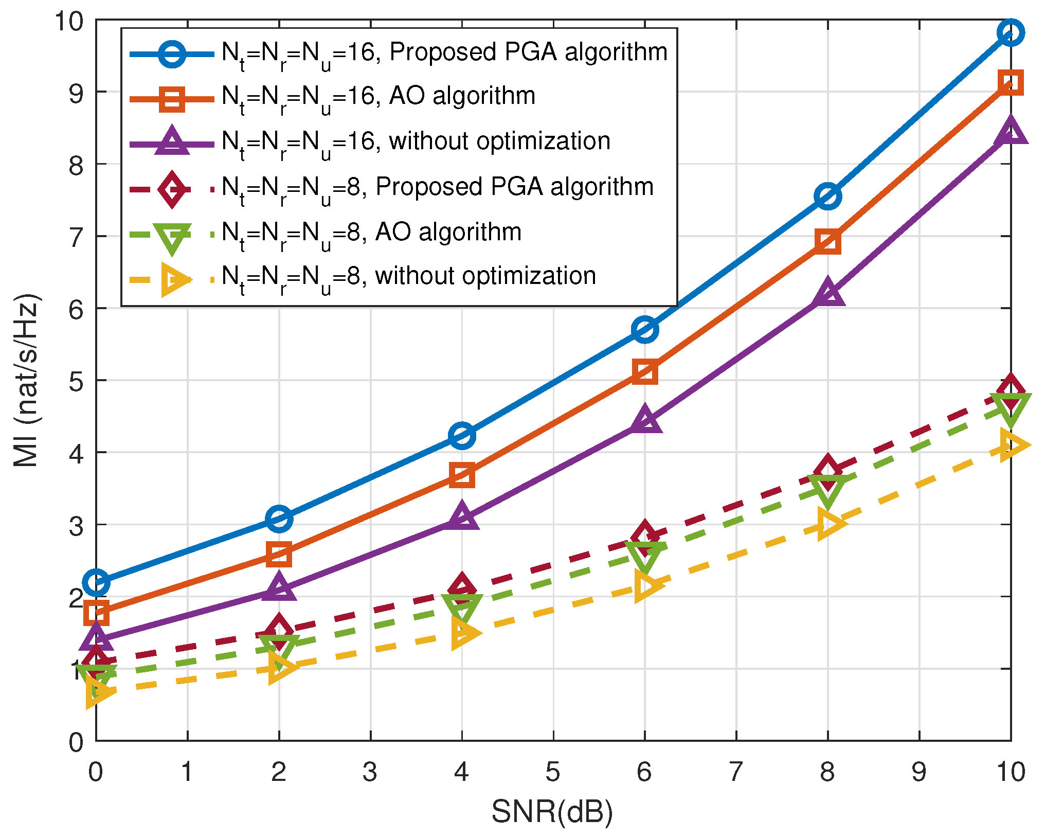
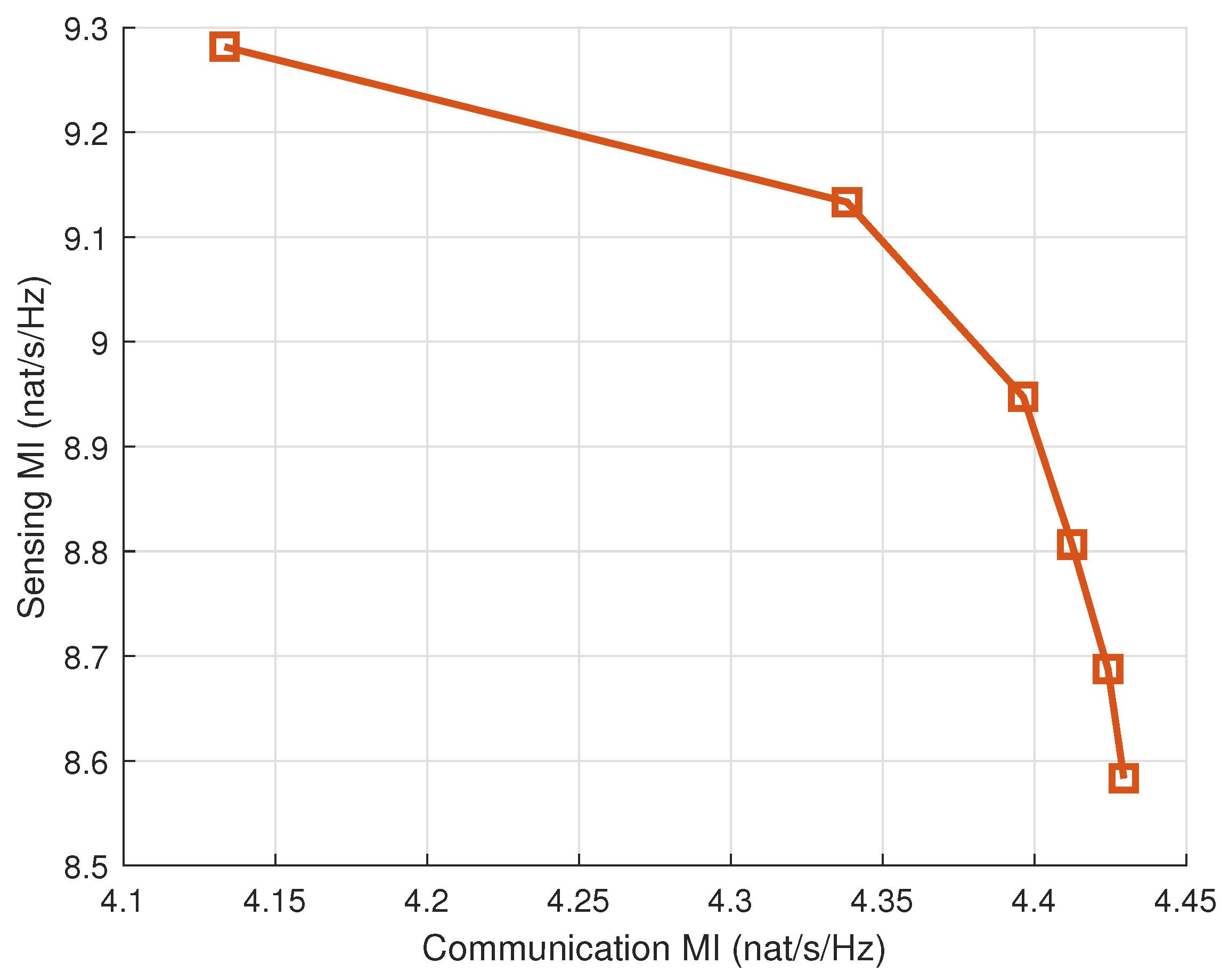
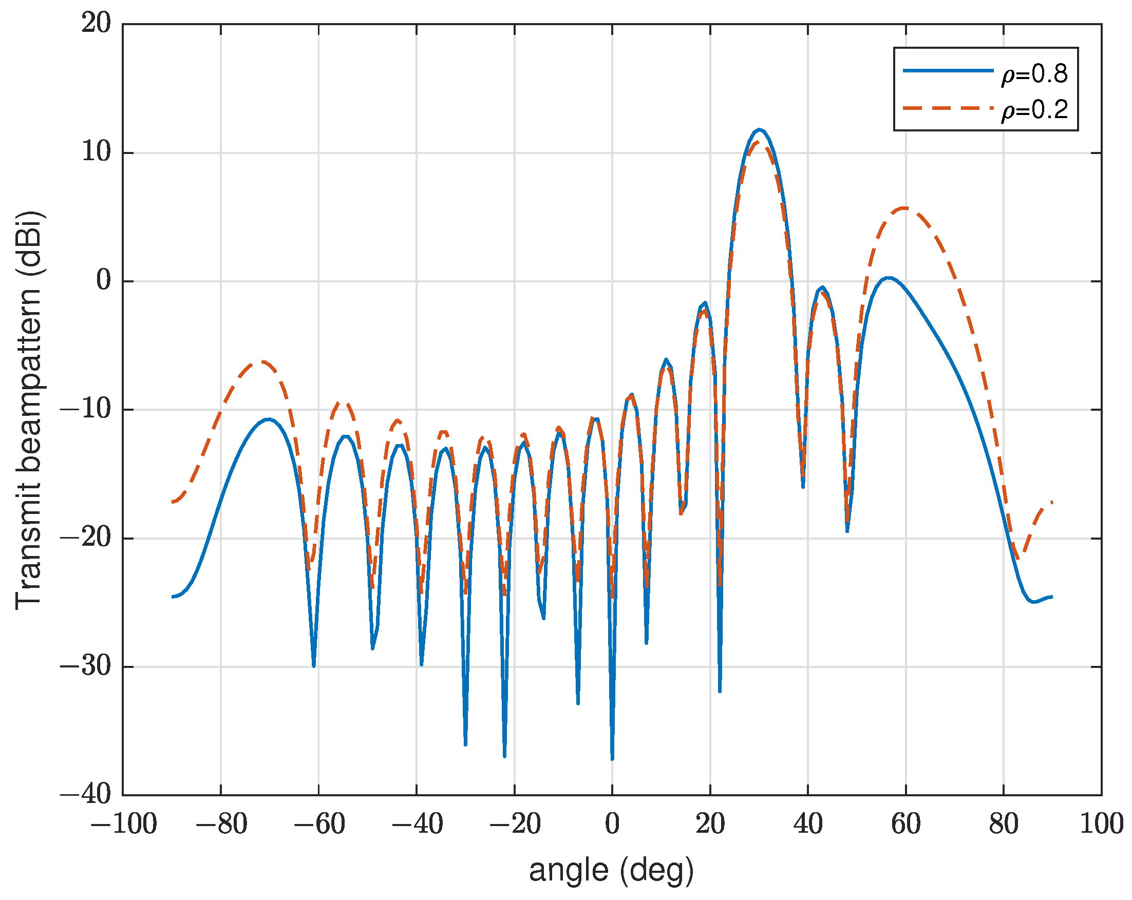
4. Numerical Results

In this section, we provide numerical results to verify the accuracy of the derived closed-form weighted MI expression and the effectiveness of the proposed PGA algorithm. The simulation results of communication MI, sensing MI, and weighted MI are generated from the Monte Carlo simulations. For the settings of the communication and sensing channels, statistical characteristics parameters of the channel, including the deterministic unitary matrices $\mathbf{U}$, $\mathbf{V}$, ${\mathbf{R}}_l$, and ${\mathbf{T}}_l$ as well as the variance matrices $\mathbf{M}$ and ${\mathbf{N}}_l$ are generated randomly but fixed in each Monte Carlo simulation. Then, the simulation results of communication MI, sensing MI, and weighted MI are averaged over ${10}^4$ channel realizations, where $\mathbf{P}$, ${\mathbf{Q}}_l$, and $\mathbf{S}$ are randomly generated. Unless otherwise stated, the number of scatterers, data streams, and signal samples are set as $L=2$, $M=N_u$, and $N_s=M$, respectively. In addition, the transmit power budget is set as $P_t=N_t$. For comprehensive performance comparison, the AO algorithm proposed in [19] is adopted as the benchmark scheme, while the beamforming matrix without optimization is set as $\mathbf{W}=\sqrt{P_t/M}{\mathbf{I}}_M$. For the proposed Algorithm 1, the convergence criterion $\epsilon$ is set as ${10}^{-3}$. It should be noted that since the radar detection link distance is typically longer than the communication link distance to UE, without loss of generality, we assume that the signal–noise ratio (SNR) at BS is 20 dB higher than the SNR at the sensing node. Furthermore, it should be noted that the SNR mentioned in this section refers to the SNR at BS.

We first verify the accuracy of the obtained closed-form MI expression for communication MI and sensing MI without optimization in Figure 2. Considering the actual deployment in [20], the number of antennas are set $N_t=N_r=N_u=16$. The solid lines represent theoretical results calculated by the communication MI expression (51) and sensing MI expression (50), respectively. On the other hand, the Monte Carlo simulation results of these MI (5) and (6) are also illustrated in Figure 2, where the markers represent the expected values of MI and the vertical bars represent the standard deviation above and below the expected values. It can be observed that the theoretical analyses match the simulation results of average MI excellently. In addition, we compare the time consumption to obtain results in Figure 2 of different methods in

Table 1. Time consumption for different schemes.

	${\mathit{N}}_{\mathit{t}}={\mathit{N}}_{\mathit{r}}={\mathit{N}}_{\mathit{u}}=8$	${\mathit{N}}_{\mathit{t}}={\mathit{N}}_{\mathit{r}}={\mathit{N}}_{\mathit{u}}=16$
Closed-form expressions	0.08 s	0.63 s
Monte Carlo simulation	5.53 s	22.12 s

. The closed-form expressions calculation and Monte Carlo simulation are both completed on a workstation equipped with an i9-10900K CPU and 32 GB of RAM. It can be observed that the efficiency of the derived closed form expression is significantly higher than that of Monte Carlo simulation.

Subsequently, the convergence of the proposed PGA algorithm under different numbers of antennas is plotted in Figure 3. The weighting factor and the SNR are set as $\rho =0.8$ and 10 dB, respectively. It can be observed that the weighted MI increases with the number of antennas. This is because a larger number of antennas provides higher diversity gain and greater design degrees of freedom (DoFs). In addition, the weighted MI increases with the iterations and converges within three iterations, demonstrating the fast convergence of the proposed PGA algorithm.

To demonstrate the effectiveness of the proposed optimization algorithm, we show the optimized weighted MI with different numbers of antennas for the considered system in Figure 4. The weighting factor is set as $\rho$ = 0.9. It can be observed that, compared with the benchmark scheme in [19] and the transmission scheme without optimization, the proposed PGA algorithm can achieve significant improvement. For instance, under the conditions of SNR = 4 dB, the proposed PGA algorithm achieves a 37% gain compared to the transmission scheme without optimization and a 14% gain over the benchmark scheme in [19]. This is because a better precoding matrix can be found through gradient optimization, which can improve the mutual information of communication and sensing while satisfying the constraints. In addition, we compare the time consumption of different optimization schemes in

Table 2. Time consumption for different optimization methods.

	${\mathit{N}}_{\mathit{t}}={\mathit{N}}_{\mathit{r}}={\mathit{N}}_{\mathit{u}}=8$	${\mathit{N}}_{\mathit{t}}={\mathit{N}}_{\mathit{r}}={\mathit{N}}_{\mathit{u}}=16$
Proposed PGA algorithm	0.54 s	1.41 s
AO algorithm [19]	7.88 s	98.76 s

, where SNR is set as 0dB. It can be observed that the efficiency of the proposed PGA algorithm is significantly higher than the benchmark scheme in [19].

To further demonstrate the effectiveness of the proposed PGA algorithm in the ultra-large MIMO regime, we present the optimized weighted MI in Figure 5, where the number of antennas is set as $N_t=N_r=130,N_u=70$, respectively. It can be observed that the proposed PGA algorithm remains effective in ultra-large MIMO regimes. Under the conditions of SNR = 10 dB, the proposed PGA algorithm achieves a 28% gain compared to the transmission scheme without optimization.

To further depict the trade-off between sensing and communication MI, we show the optimized weighted MI with weighting factors $\rho$ ranging from 0 to 1 in Figure 6. The number of antennas and the SNR are set as $N_t=N_r=N_u=8$ and 10 dB, respectively. As the weighting factor increases, the ISAC system places greater emphasis on sensing performance, and conversely, prioritizes communication performance when the weighting factor decreases.

We present the transmit beampattern generated by the proposed PGA algorithm in Figure 7, where BS and the center of the scatterers are located at ${60}^{\circ }$ and ${30}^{\circ }$, respectively. It can be observed that with the weighting factor $\rho$ increasing, the transmit beams are more concentrated at the direction of the scatterers, thereby enhancing the sensing performance. This is still because with a higher weighting factor, the proposed algorithm tends to focus more on the sensing MI.

5. Conclusions

In this paper, we investigated the beamforming design for a practical MIMO ISAC system. To derive the closed-form expression of the weighted MI for the considered system, we resorted to the operator-valued free probability. Based on the closed-form expression, we proposed the PGA algorithm to design the transmit beamforming matrix for maximizing the weighted MI. Simulation results verified the accuracy of the derived closed-form expression and the effectiveness of the proposed algorithm. In addition, our proposed method can be further applied to smart vehicular networks, smart factories, and UAV scenarios, which allows them to share information (communication) while scanning the surroundings (sensing) using the same hardware.

References

1. Zhang, J.A.; Rahman, M.L.; Wu, K.; Huang, X.; Guo, Y.J.; Chen, S.; Yuan, J. Enabling joint communication and radar sensing in mobile networks—A Survey. IEEE Commun. Surv. Tutor. 2022, 24, 306–345. [Google Scholar] [CrossRef]
2. Liu, F.; Masouros, C.; Li, A.; Sun, H.; Hanzo, L. Mu-MIMO communications with MIMO radar: From co-existence to joint transmission. IEEE Trans. Wirel. Commun. 2018, 7, 2755–2770. [Google Scholar] [CrossRef]
3. Liu, F.; Liu, Y.; Li, A.; Eldar, C.M.Y. Cramér-Rao bound optimization for joint radar-communication beamforming. IEEE Trans. Wirel. Commun. 2022, 70, 240–253. [Google Scholar] [CrossRef]
4. Liu, R.; Li, M.; Li, Q.; Swindlehurst, A. SNR/CRB-constrained joint beamforming and reflection designs for RIS-ISAC systems. IEEE Trans. Wirel. Commun. 2024, 7, 7456–7470. [Google Scholar] [CrossRef]
5. Wang, X.; Fei, Z.; Zhang, J.A.; Xu, J. Partially-connected hybrid beamforming design for integrated sensing and communication systems. IEEE Trans. Commun. 2022, 70, 6648–6660. [Google Scholar] [CrossRef]
6. Al-Jarrah, M.; Alsusa, E.; Masouros, C. A unified performance framework for integrated sensing-communications based on KL-divergence. IEEE Trans. Wirel. Commun. 2023, 22, 9390–9411. [Google Scholar] [CrossRef]
7. Fei, Z.; Tang, S.; Wang, X. Revealing the Trade-Off in ISAC Systems: The KL Divergence Perspective. IEEE Wirel. Commun. Lett. 2024, 13, 2747–2751. [Google Scholar] [CrossRef]
8. Li, J.; Zhou, G.; Gong, T.; Liu, N. A Framework for Mutual Information-Based MIMO Integrated Sensing and Communication Beamforming Design. IEEE Trans. Veh. Technol. 2024, 73, 8352–8366. [Google Scholar] [CrossRef]
9. Piao, J.; Wei, Z.; Yuan, X.; Yang, X.; Wu, H.; Feng, Z. Mutual Information Metrics for Uplink MIMO-OFDM Integrated Sensing and Communication System. In Proceedings of the GLOBECOM 2023—2023 IEEE Global Communications Conference, Kuala Lumpur, Malaysia, 4–8 December 2023; pp. 7387–7392. [Google Scholar]
10. Huang, X.; Zhang, J.; Xia, W.; Cai, S.; Fan, F.; Yuen, C. Statistical CSI Assisted Beamforming for Co-Existence of MIMO Radar and MIMO Communication System. IEEE Trans. Veh. Technol. 2025. [CrossRef]
11. Weichselberger, W.; Herdin, M.; Ozcelik, H.; Bonek, E. A stochastic MIMO channel model with joint correlation of both link ends. IEEE Trans. Wirel. Commun. 2006, 5, 90–100. [Google Scholar] [CrossRef]
12. Xu, Y.; Li, Y.; Zhang, J.A.; Di Renzo, M.; Quek, T.Q. Joint beamforming for RIS-assisted integrated sensing and communication systems. IEEE Trans. Commun. 2024, 72, 2232–2246. [Google Scholar] [CrossRef]
13. Tulino, A.M.; Verdu, S. Random matrix theory and wireless communications. Found. Trends Commun. Inf. Theory 2004, 1, 1–18. [Google Scholar] [CrossRef]
14. Hoydis, J.; Couillet, R.; Debbah, M. Asymptotic analysis of double-scattering channels. In Proceedings of the 2011 Conference Record of the Forty Fifth Asilomar Conference on Signals, Systems and Computers (ASILOMAR), Pacific Grove, CA, USA, 6–9 November 2011; pp. 1935–1939. [Google Scholar]
15. Silverstein, J.W. Strong convergence of the empirical distribution of eigenvalues of large dimensional random matrices. J. Multivar. Anal. 1995, 55, 331–339. [Google Scholar] [CrossRef]
16. Belinschi, S.T.; Mai, T.; Speicher, R. Analytic subordination theory of operator-valued free additive convolution and the solution of a general random matrix problem. J. Reine Angew. Math. (Crelles J.) 2017, 2017, 21–53. [Google Scholar] [CrossRef]
17. Muller, R.R. On the asymptotic eigenvalue distribution of concatenated vector-valued fading channels. IEEE Trans. Inf. Theory 2002, 48, 2086–2091. [Google Scholar] [CrossRef]
18. Zheng, Z.; Wang, S.; Fei, Z.; Sun, Z.; Yuan, J. On the mutual information of multi-RIS assisted MIMO: From operator-valued free probability aspect. IEEE Trans. Commun. 2023, 71, 6952–6966. [Google Scholar] [CrossRef]
19. Wang, S.; Zheng, Z.; Fei, Z.; Wang, X.; Guo, J. Analysis and Optimization of Multi-RIS-Assisted Dual-Functional Radar-Communication Systems via Free Probability Theory. In Proceedings of the GLOBECOM 2023—2023 IEEE Global Communications Conference, Kuala Lumpur, Malaysia, 4–8 December 2023; pp. 6505–6510. [Google Scholar]
20. Behdad, Z.; Demir, Ö.; Sung, K.; Björnson, E.; Cavdar, C. Multi-Static Target Detection and Power Allocation for Integrated Sensing and Communication in Cell-Free Massive MIMO. IEEE Trans. Wirel. Commun. 2024, 23, 11580–11596. [Google Scholar] [CrossRef]
21. Wang, S.; Zheng, Z.; Fei, Z.; Guo, J.; Yuan, J.; Sun, Z. Toward Ergodic Sum Rate Maximization of Multiple-RIS-Assisted MIMO Multiple Access Channels Over Generic Rician Fading. IEEE Trans. Wirel. Commun. 2024, 23, 9613–9628. [Google Scholar] [CrossRef]
22. Horn, R.; Johnson, C. Matrix Analysis; Cambridge University Press: New York, NY, USA, 2013. [Google Scholar]
Figure 1. Considered MIMO ISAC system.
Electronics 14 02515 g001
Figure 2. Communication MI and sensing MI versus SNR.
Electronics 14 02515 g002
Figure 3. Weighted MI versus the number of iterations, where ρ = 0.8 .
Electronics 14 02515 g003
Figure 4. Weighted MI versus SNR with different schemes, where ρ = 0.9 and ’AO algorithm’ was proposed in [19].
Electronics 14 02515 g004
Figure 5. Weighted MI versus SNR in the ultra-large MIMO regim, where ρ = 0.9 .
Electronics 14 02515 g005
Figure 6. Sensing MI versus communication MI.
Electronics 14 02515 g006
Figure 7. Transmit beampattern generated by PGA algorithm.
Electronics 14 02515 g007